Diversity and Economic Performance in a Model with Progressive Taxation

Munich Personal RePEc Archive

Diversity and Economic Performance in

a Model with Progressive Taxation

Wang, Wei and Suen, Richard M. H.

Southwestern University of Finance and Economics, University of

Leicester

23 July 2018

Diversity and Economic Performance in a Model with

Progressive Taxation

Wei Wang

Richard M. H. Suen

This Version: 23rd July, 2018.

Abstract

Is a more heterogeneous population bene…cial or harmful to long-term economic

perfor-mance? This paper addresses this and other questions in a dynamic general equilibrium model

where consumers have di¤erent labour productivity and time preference. We show how

dif-ferences in the cross-sectional distribution of these characteristics can a¤ect the economy via

two channels. The …rst one involves changing the composition of the labour force; and the

second one involves changing the cross-sectional distribution of marginal tax rate. We show

how these channels are, respectively, determined by the shape of the labour supply function

and the curvature of the marginal tax function.

Keywords: Consumer Heterogeneity, Progressive Taxation, Endogenous Labour Supply.

JEL classi…cation: D31, E62.

Research Institute of Economics and Management, Southwestern University of Finance and Economics, Gezhi Building 1205, Liulin Campus, Chengdu, Sichuan, P. R. China, 611130. Email: [email protected]

y_{Corresponding Author: School of Business, Economics Division, University of Leicester, Leicester LE1 7RH,}

1

Introduction

Is a more heterogeneous population bene…cial or harmful to long-term economic performance?

What role does redistributive policy, such as progressive taxation, play in this matter? This

paper addresses these questions using a dynamic general equilibrium model with heterogeneous

consumers. In particular, the consumers are ex ante di¤erent in their labour productivity and

time preference.1 Our goal is to analyse how di¤erences in the cross-sectional distribution of these

characteristics a¤ect long-term economic outcomes.

The economic implications of diversity have long been a subject of empirical research.2 Several

recent studies have provided evidence on the positive e¤ect of ethnic and cultural diversity on

productivity and economic growth (e.g., Ottaviano and Peri, 2006; Ager and Brückner, 2013;

Traxet al., 2015; Alesinaet al., 2016).3 _{In contrast, there has been very few theoretical research}

on this timely and important issue. This lack is somewhat surprising, given the prominence

of heterogeneous-agent models in macroeconomics. The present study makes the …rst attempt to

examine the issue of diversity using this type of model. Speci…cally, we adopt a similar deterministic

neoclassical framework as in Sarte (1997), Li and Sarte (2004), Carroll and Young (2009, 2011) and

Angyridis (2015). In these models, ex ante heterogeneity is the root cause of income and wealth

inequality.4 Progressive taxation comes into play by distorting prices and incentives, which in turn

in‡uences howex ante heterogeneity translates intoex post economic inequality. The distribution

of consumer types is typically taken as invariant in these previous studies. Thus, the e¤ects of its

changes are largely unexplored. The present study is intended to …ll this gap.

The main points of this paper can be explained in terms of two types of e¤ects, namely

compo-sition e¤ects and general equilibrium e¤ects. The former refers to changes in aggregate quantities

due to changes in the composition of the underlying population, while the latter refers to changes

1_{Time preference heterogeneity has been previously considered in Sarte (1997), Li and Sarte (2001), Carroll and}

Young (2011), Suen (2014) and Angyridis (2015) among others. The empirical evidence on this type of heterogeneity has been reviewed in Fredericket al. (2002). We are agnostic about the source of consumer heterogeneity, which can be due to racial, cultural, physiological or other reasons. Throughout this paper, we will treat the terms “diversity” and “ex ante heterogeneity” as synonymous.

2_{For extensive survey of this literature, see Alesina and La Ferrara (2005) and Alesinaet al. (2016).}

3_{The analysis in Ottaviano and Peri (2006), Ager and Brückner (2013) and Trax et al. (2015) are based on}

micro-level data from developed countries, such as Germany and the United States. Alesinaet al. (2016), on the other hand, conduct cross-country comparisons using aggregate level data from 195 countries. Other cross-country studies, such as Easterly and Levine (1997) and Collier and Gunning (1999), focus on African countries and …nd a negative relation between ethnic diversity and economic growth.

4_{Implicitly, it is assumed that there is perfect consumption insurance so that individuals’ choices are una¤ected}

in individual-level quantities caused by the adjustment in equilibrium prices.5 _{The exact nature}

of these e¤ects depend on the type of heterogeneity considered. In the case of labour productivity

heterogeneity, these e¤ects primarily take place in the labour market. Speci…cally, any changes

in the cross-sectional distribution of labour productivity will alter the composition of the labour

force. This induces a shift in the aggregate labour supply function, thus triggering an adjustment

in equilibrium wage rate (and interest rate), and in turn a¤ects individuals’ labour supply decision.

Using general speci…cations of utility function, production function and progressive tax function,

we derive conditions under which a more dispersed distribution of labour productivity will give

rise to a higher level of aggregate labour supply and aggregate output in the steady state. Under

these conditions, greater diversity will also bene…t individual consumers by boosting their pre-tax

income and consumption.

The case of time preference heterogeneity is more complicated due to the following reasons.

Firstly, any changes in the cross-sectional distribution of time preference will not only a¤ect the

composition of the labour force, but also the cross-sectional distribution of pre-tax incomes; and

these two changes often have con‡icting e¤ects on equilibrium prices. Secondly, the composition

e¤ect on aggregate labour supply is now more di¢cult to determine due to an income e¤ect on

individual labour supply. In light of these di¢culties, the analysis of time preference heterogeneity

is divided into three steps. First, in Section 4.1 we consider a simpli…ed model in which labour

supply is perfectly inelastic. This essentially shuts down the e¤ect of time preference heterogeneity

on aggregate labour supply. We then focus on how changing the distribution of time preference

will a¤ect the cross-sectional distribution of pre-tax income and marginal tax rates.6 In the

con-text of representative-agent models, the negative relation between marginal tax rate and capital

accumulation is well understood: lowering the marginal tax rate can promote capital accumulation

by raising the after-tax return on savings.7 In this paper, we show that changing the

distribu-tion of time preference can have a similar e¤ect on capital accumuladistribu-tion, even when there is no

change in the tax function itself. The exact outcome of this is determined by the curvature of

5_{If we think of aggregate variables (e.g., aggregate consumption expenditure) as a weighted sum of the}

correspond-ing micro-level variables (e.g., household consumption expenditure), then the composition e¤ect refers to changes in the weights while the general equilibrium e¤ect concerns changes in the value of the micro-level variables.

6_{Since the tax function is assumed to be continuously di¤erentiable, striclty increasing and strictly convex, there}

exists a one-to-one mapping between pre-tax income and marginal tax rate. Hence, the distribution of these two variables are isomorphic.

7_{Empirical evidence on this is scant, however, mainly because of the di¢culty in measuring marginal tax rate.}

themarginal tax function, which is an often overlooked feature of the tax function.8 _{Speci…cally,}

if the marginal tax function is concave, then a mean-preserving but more dispersed distribution

of time preference will lead to a lower average marginal tax rate and a higher level of capital

accumulation. The opposite is true if the marginal tax function is convex. The intuition of these

results can be explained as follows: Start with a homogeneous economy in which all consumers are

ex ante identical and have the same pre-tax income. Suppose now a mean-preserving dispersion

in time preference is introduced. This will create a non-degenerate distribution in pre-tax income

and marginal tax rate. In particular, the relatively poor consumers in the heterogeneous economy

will pay a lower marginal tax rate than in the homogeneous world, and the relatively rich will

pay a higher rate. The shape of the marginal tax function matters when it comes to aggregation.

If the marginal tax function is concave, then the decrease in marginal tax rate among the poor

will outweigh the increase among the rich. As a result, the heterogeneous economy will have a

lower average marginal tax rate than the homogeneous economy.9 Our main results in Section

4.1 generalise this comparison to two heterogeneous economies and provide the conditions under

which greater diversity is bene…cial or harmful to capital accumulation. Next, in Section 4.2 we

resume the assumption of elastic labour supply but abstract away from the income e¤ect. This is

achieved by using the so-called “no-income-e¤ect” utility function. In this case, the e¤ect of time

preference heterogeneity on aggregate labour supply can be easily characterised. In particular, if

the marginal rate of substitution (MRS) between consumption and labour is a convex (or concave)

function, then a mean-preserving spread in the distribution of time preference will lead to a

down-ward (or updown-ward) shift in the aggregate labour supply function. Finally, in Section 4.3 we provide

some numerical examples to illustrate the composition e¤ects and the general equilibrium e¤ects

in the full version of the model, where the income e¤ect on labour supply is operative. Under some

plausible parameter values, we …nd that a mean-preserving dispersion in time preference has only a

mild positive e¤ect on the capital-labour ratio (and hence the equilibrium prices), but a signi…cant

negative impact on aggregate labour supply. The latter is the result of a negative composition

e¤ect on the labour force.

The rest of the paper is organised as follows: Section 2 presents the baseline model. Section 3

analyses the e¤ects of greater labour productivity heterogeneity. Section 4 focuses on the e¤ects

8_{If a tax function ( )is thrice di¤erentiable, then the corresponding marginal tax function is concave (or convex)}

if and only if the third-order derivative 000_{( )is negative (or positive). It is important to note that almost all the} existing quantitative studies on progressive taxation have adopted a speci…cation which implies a concave marginal tax function (see Section 4.1 for details). But the relation between this and the distribution of marginal tax rates has not been previously reported.

of time preference heterogeneity. Section 5 concludes.

2

The Baseline Model

2.1 Consumers

Time is discrete and is denoted byt2 f0;1;2; :::g:Consider an economy inhabited by a continuum

of in…nitely-lived consumers with di¤erent rate of time preference and labour productivity. The

size of population is constant over time and is normalised to one. Let _i >0 be the rate of time

preference of the ith consumer, i2[0;1]; and "i >0 his labour productivity. Both are

predeter-mined and constant over time. The joint distribution of these characteristics across consumers is

given byH( ; "); which is de…ned on the support ; ["; "]; with > > 0 and " > " > 0:

This distribution can be either discrete or continuous (or mixed). The marginal distribution of

and "are, respectively, denoted byH1( ) andH2("):

In each time period, each consumer has one unit of time which can be divided between labour

and leisure. Letni;t andli;t denote, respectively, the fraction of time spent on working and leisure

activities by theith consumer at timet: These variables are subject to the following constraints:

ni;t 2[0;1]; li;t 2[0;1]; and ni;t+li;t = 1: (1)

There is a single commodity in this economy which can be used for consumption and investment.

Let ci;t be the consumption of the ith consumer at time t: All consumers have preferences over

sequences of consumption and labour hours which can be represented by

1

X

t=0

t

iU(ci;t; ni;t); (2)

where _i (1 + _i) 1 is the subjective discount factor of the ith consumer and U( ) is the

(per-period) utility function. The latter is identical for all consumers and has the following properties.

Assumption A1 The utility function U :R+ [0;1]! R is twice continuously di¤erentiable,

strictly increasing in c, strictly decreasing in n and jointly strictly concave in (c; n): For every

n2[0;1];there existsc(n) 0 such thatUc(c; n)! 1 asc!c(n):

Assumption A2 The marginal rate of substitution (MRS) between consumption and labour,

The last part of Assumption A1 is similar in spirit to the Inada condition on the utility function.

Speci…cally,c(n) 0can be interpreted as a subsistence level of consumption (which may depend

on n). When a consumer is close to subsistence, the marginal utility of consumption will become

in…nitely large. Thus, the consumer will never choose to consume at c(n): Assumption A2, on

the other hand, ensures that consumption and leisure are both normal goods.10 This assumption

is equivalent to

Ucn(c; n)

Un(c; n)

Uc(c; n)

Ucc(c; n) and Unn(c; n)<

Un(c; n)

Uc(c; n)

Ucn(c; n);

for all (c; n): Both assumptions are satis…ed by a large set of utility functions, including (i) the

additively separable speci…cation,

U(c; n) = c

1 ₁

1 A

n1+

1 + ;

with > 0; A > 0 and > 0; (ii) the “no-income-e¤ect” utility function or GHH preferences,

named after the work of Greenwood et al. (1988),

U(c; n) = c An

1+ 1 ₁

1 ; (3)

with >0; A >0 and >0; and (ii) the homothetic utility function,

U(c; n) =

h

c (1 n)1 i1 1

1 ; (4)

with 1 and 2 (0;1):11 For the additively separable and the homothetic speci…cations,

the subsistence level of consumption in Assumption A1 is identical to zero, i.e., c(n) = 0 for

all n: For GHH preferences, we set c(n) An1+ since the marginal utility of consumption

Uc(c; n) = c An1+ becomes in…nite whenc tends toAn1+ :

Next, we turn to consider the consumers’ budget constraint. Let wt be the wage rate for an

e¤ective unit of labour at timet: Then consumer i’s labour income at time tis given by wt"ini;t:

Consumers can save and borrow through a single risk-free asset. Letai;t denote consumeri’s asset

1 0_{This means, holding other things constant, an increase in non-wage income in the current period will lead to an}

increase in current consumption and a decrease in current labour supply. This normality assumption is commonly used in existing studies. See for instance, Nourry (2001) and Dattaet al. (2002).

1 1_{By setting = (1 +&)} 1

and = 1 1₍₁

e);we can rewrite (4) asU(c; n) = [c(1 n)&_]1 e_{=(1 e);}

holdings at the beginning of timet: The consumer is in debt if this falls below zero. The interest

income (or interest payment) associated with these assets is given byrtai;t;wherertis the interest

rate. The sum of labour income and interest income, denoted byyi;t wt"ini;t+rtai;t;is subject

to a progressive tax schedule ( ).12 The properties of the tax function are summarised below:

Assumption A3 The function :R+!R+is continuously di¤erentiable and strictly increasing.

The marginal tax rate is zero at the origin, i.e., 0(0) = 0; strictly increasing for all y 0 and

satis…es lim

y!1

0_{(y) = 1:}

The assumption of an increasing marginal tax rate is often referred to as marginal rate

pro-gressivity. If (0) 0;then marginal rate progressivity is equivalent to average rate progressivity,

i.e., average tax rate (y)=y is increasing in y: A negative value of (0) can be interpreted as a

lump-sum transfer from the government. Conversely, a positive (0)can be viewed as a lump-sum

tax appended to the progressive tax schedule. In this case, the average tax rate is non-monotonic

iny.13

Consumer i’s budget constraint at timet can be expressed as

ci;t+ai;t+1 ai;t =yi;t (yi;t): (5)

Taking prices and tax schedule as given, each consumer chooses a sequence of consumption, leisure,

labour and asset holdings so as to maximise his lifetime utility in (2), subject to the time-use

constraints in (1), the sequential budget constraint in (5) and the initial amount of assetsa0 >0.14

There is no other restriction on borrowing except the no-Ponzi-scheme condition, which is implied

by the transversality condition stated below. The solution of the consumer’s problem is completely

characterised by the sequential budget constraint in (5); the Euler equation for consumption

Uc(ci;t; ni;t) = iUc(ci;t+1; ni;t+1) 1 + 1 0(yi;t+1) rt+1 ; (6)

1 2_{This setup, which is commonly used in existing studies, implicitly assumes that interests paid on loans are tax}

deductible. This assumption is adopted mainly for analytical convenience. In most countries, interests paid on personal loans are in general not deductible from taxes. In the United States, for instance, taxpayers can claim deductions on interests paid on student loans and residential mortgages but not on other types of loans (such as credit card debts).

1 3_{The sign of (0)is immaterial for all of our theoretical results.}

1 4_{The current framework can be easily extended to allow for heterogeneity in initial wealth. But since we focus}

the optimality condition for labour supply

(ci;t; ni;t) wt"i 1 0(yi;t)

8 > > > > < > > > > :

0 ifni;t = 0;

= 0 ifni;t 2(0;1);

0 ifni;t = 1;

(7)

and the transversality condition

lim

T!1

8 < :

"_T

Y

t=1

1 +'_i;t

# 1

ai;T+1

9 =

;= 0;

where'_i;t [1 0_(y

i;t)]rt is the after-tax interest rate. The conditions in (7) take into account

the possibility of corner solution for ni;t:For instance, it is optimal to haveni;t= 0 if the relative

price of leisure, i.e.,wt"i[1 0(yi;t)];is less than or equal to the MRS atni;t = 0;i.e., (ci;t;0):

2.2 Production and Government

On the supply side of the economy, there is a large number of identical …rms. In each time period,

each …rm hires labour and rents physical capital from the competitive factor markets, and produces

output using a neoclassical production function: Yt=F(Kt; Nt);whereYtdenotes output at time

t; KtandNtdenote capital input and labour input, respectively. The properties of the production

function are summarised below.

Assumption A4 The production function F : R2+ ! R+ is twice continuously di¤erentiable,

strictly increasing and strictly concave in(K; N):It also exhibits constant returns to scale (CRTS)

in the two inputs and satis…es the Inada conditions.

Since the production function exhibits CRTS, we can focus on the pro…t-maximisation problem

of a single representative …rm. Let Rt be the rental price of physical capital at timet. Then the

representative …rm’s problem is

max

Kt;Nt

fF(Kt; Nt) wtNt RtKtg;

and the …rst-order conditions are Rt = FK(kt;1) and wt = FN(kt;1); where kt Kt=Nt is the

capital-labour ratio at timet:

government purchases(Gt):This spending is called unproductive because it has no direct impact

on the consumers’ well-being and the production of goods. The government’s budget constraint

at any timetis given by

Z 1

0

(yi;t)di=Gt; for all t 0: (8)

2.3 Competitive Equilibrium

Given a progressive tax schedule, a competitive equilibrium consists of sequences of allocations

fci;t; li;t; ni;t; ai;tg_t1₌₀ for each i 2 [0;1]; aggregate inputs fKt; Ntg1t=0; prices fwt; rt; Rtg1t=0 and

government spending fGtg1t=0 such that

(i) Given prices, fci;t; li;t; ni;t; ai;tg1_t=0 solves consumer i’s problem.

(ii) Given prices,fKt; Ntg1t=0 solves the representative …rm’s problem in every time period.

(iii) The government’s budget is balanced in every time period.

(iv) All markets clear in every time period, so that

Kt=

Z 1

0

ai;tdi; and Nt=

Z 1

0

"ini;tdi; for all t 0:

We con…ne our attention to stationary equilibria or steady states of this economy. These can

be characterised as follows: For any non-trivial steady state with capital-labour ratio k > 0; let

w(k) and r(k) be the corresponding wage rate and interest rate. To highlight the dependence

of individual choices on ( ; "); we use y(k; ; "); c(k; ; "); a(k; ; ") and n(k; ; ") to denote,

respectively, the pre-tax income, consumption, asset holdings and labour supply of a type-( ; ")

consumer in this steady state (the subscriptiwill be omitted from this point on). These

individual-level variables are completely determined by

=r(k) 1 0[y(k; ; ")] ; (9)

c(k; ; ") =y(k; ; ") [y(k; ; ")]; (10)

a(k; ; ") = y(k; ; ") w(k)"n(k; ; ")

[c(k; ; "); n(k; ; ")] w(k) r(k)"

8 > > > > < > > > > :

0 ifn(k; ; ") = 0;

= 0 ifn(k; ; ")2(0;1);

0 ifn(k; ; ") = 1:

(12)

Equation (9) is obtained by setting Uc(ci;t; ni;t) = Uc(ci;t+1; ni;t+1) in the Euler equation of

consumption.15 The intuition behind this equation is as follows: In any stationary equilibrium, each

consumer will maintain a constant level of marginal utility of consumption across time. This can be

achieved if and only if the after-tax interest rate is equal to the consumer’s rate of time preference.

Such parity has two implications. Firstly, consumers with the same rate of time preference will

face the same marginal tax rate and have the same level of pre-tax income, regardless of their

labour productivity. In other words, y(k; ; ") is independent of ": Secondly, for any in ; ;

y(k; )is a strictly decreasing function ink:This is due to the following mechanism: Holding other

things constant, an increase in k will lower the pre-tax interest rate and create an incentive for

the consumer to substitute future consumption for current consumption. In order to maintain a

constant marginal utility of consumption, it is necessary for the marginal tax rate to fall so as to

maintain the equality in (9). Since 0( )is strictly increasing, this leads to a lower level of pre-tax

income for all : In the sequel, we will refer to this as the intertemporal smoothing e¤ect. Note

that this e¤ect arises only when the income tax schedule is nonlinear.16 _{Equation (10) is obtained}

by setting ai;t+1 = ai;t in the sequential budget constraint. This, together with (9), implies that

c(k; ; ") is also independent of ": Equation (11) follows from the de…nition of pre-tax income.

Equation (12) is obtained by substituting (9) into (7).

We now derive a single equation that can help determine the steady-state value ofk:To start,

de…ne : [0; ]!R+[ f+1gas the inverse function of 0_{( ), i.e., [} 0_{(y)] =y for ally 0:Since}

the marginal tax function is continuous and strictly increasing, ( )is a single-valued, continuous,

1 5_{Note that equation (9) is valid even if (i) there isex ante heterogeneity in the utility function, i.e.,U}i

(c; n)6=

Uj_{(c; n)for somei6=jin [0;1];and (ii) there is no disutility from labour, i.e.,U(c; n}

1) =U(c; n2)for alln16=n2

in[0;1]and for allc 0:

1 6_{If the income tax function is linear, i.e.,} 0_{(y) =}

strictly increasing function. Using (9) and the de…nition of pre-tax income, we can write

y(k; ) 1

r(k) =w(k)"n(k; ; ") +r(k)a(k; ; "): (13)

Integrating both sides of (13) across all types of consumers yields

Y (k)

Z 1

r(k) dH1( ) = [f(k) k]N(k); (14)

whereH1( )is the marginal distribution of ;N(k) is the aggregate labour supply, de…ned as

N(k)

Z Z "

"

"n(k; ; ")dH( ; ") ;

and f(k) F(k;1) is the reduced-form production function. Equation (14) is essentially an

accounting identity which states that the sum of all individuals’ income equals national income

(aggregate output minus depreciation of capital). We will refer to Y ( ) as the national income

function. A unique, non-trivial steady state exists if equation (14) has a single, strictly positive

solution. The rest of this section is devoted to establishing the existence of such a solution.

The …rst step is to specify the range of plausible values ofk:Since ( )is only de…ned on[0; ];

equations (13) and (14) are satis…ed only if

1

r(k) 0;

for all 2 ; :In other words, anyk that solves (14) must satisfy

1 r(k) :

To ensure that this range is nonempty, it is necessary to have >(1 ) :By the strict concavity

of f( ) and the Inada conditions on the production function, there exists a unique pair of values

kmax> kmin >0such that

r(kmax) f0(kmax) = and r(kmin) =

1 : (15)

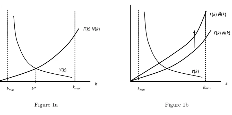
Y(k)

kmax k kmin

Γ(k)N(k)

k*

Figure 1a

Y₍k₎

k_max k k_min

Γ(k)Ñ(k)

Γ(k)N(k)

Figure 1b

Lemma 1 provides a set of necessary and su¢cient conditions under which a unique non-trivial

steady state exists in the baseline model. All proofs can be found in the Appendix. A graphical

illustration of the unique steady state is shown in Figure 1a.17

Lemma 1 Suppose Assumptions A1-A4 and > (1 ) are satis…ed. Then a unique steady

state with capital-labour ratio k 2(kmin; kmax) exists if and only if

N(kmax) [f(kmax) kmax]>

Z

1 dH1( ); (16)

and

N(kmin) [f(kmin) kmin]<

Z

1 (1 ) dH1( ): (17)

3

Heterogeneity in Labour Productivity

We now turn to the main subject of this paper, which is the economic consequences of greater

consumer heterogeneity. In the current section, we focus on the e¤ects of labour productivity

heterogeneity. The e¤ects of time preference heterogeneity will be examined in Section 4. In both

sections, we assume that"and are statistically independent in the population so thatH( ; ") =

H1( )H2(") for all ( ; "): We then compare two economies that have the same fundamentals

except for one of the marginal distributions.

1 7_{The inequalities in (16) and (17) are technical conditions which ensure that the two curves in Figure 1a cross at}

Two criteria will be used to compare di¤erent marginal distributions. The …rst one is the

Lorenz dominance criterion (also known as Lorenz order or convex order), which is commonly

used in studies of risk and inequality. Let Q( ) and Qe( ) be two distribution functions de…ned on

the same support in R+ and have the same mean. Then Qe( ) is said to be “more unequal” than

Q( ) under the Lorenz dominance criterion if

Z x

0

e

Q(z)dz

Z x

0

Q(z)dz; for all x 0: (18)

The “more unequal” distribution Qe( )is also called a mean-preserving spread of Q( ):It is

well-known that (18) is satis…ed if and only if

Z 1

0

(z)dQe(z)

Z 1

0

(z)dQ(z)

for any convex function :R+ !R;provided that the integrals exist. Intuitively, a “more unequal”

distribution of consumer characteristic is one that exhibits greater cross-sectional variations, and

thus represents a larger extent of consumer heterogeneity.

Another criterion that we use is the starshaped order. Recall that a function : R+ ! R is

starshaped if (0) 0and (z)=zis non-decreasing in z:Then Qe( ) is said to be “more unequal”

thanQ( )according to the starshaped order if

Z 1

0

(z)dQe(z)

Z 1

0

(z)dQ(z) (19)

for all bounded, continuous and starshaped function :18 The condition in (19) can be equivalently

stated as19

Z 1

x

zdQe(z)

Z 1

x

zdQ(z); for allx 0: (20)

If Q( ) and Qe( ) have the same mean (or aggregate), i.e., R₀1zdQe(z) = R₀1zdQ(z) S, then

(20) can be equivalently stated as

R1

x zdQe(z)

R1

0 zdQe(z)

R1

x zdQ(z)

R1

0 zdQ(z)

; for all x 0:

The expression on the right side of this inequality gives the fraction of the aggregate S that

is concentrated in the interval [x;1) under Q( ): The expression on the left can be similarly

interpreted. Thus, a mean-preserving but “more unequal” distribution under the starshaped order

is one that is more concentrated on the top end of the support. The relation between these two

types of order is as follows: If Q( ) and Qe( ) have the same mean and satisfy (20), thenQe( ) is

also “more unequal” than Q( ) under the Lorenz order. But the converse of this is not true in

general. Thus, the starshaped order is stronger than the Lorenz order. The rationale for using this

stronger order will be explained below.

Consider two economies that have the same size of population, utility functionu( );production

technology F( ), progressive tax schedule ( ) and distribution of time preference H1( ) de…ned

on ; :20 _{The only di¤erence between them lies in the marginal distribution of labour}

produc-tivity, which are denoted by H2(") and He2("):Both of them are de…ned on ["; "]and satisfy the

assumption stated below. The second part of Assumption A5 ensures that a unique non-trivial

steady state exists in both economies.

Assumption A5 (i) The average value of "is identical under H2( ) and He2( ). (ii) Conditions

(16) and (17) are satis…ed in both economies.

Notice that when k is held constant, changing the distribution of " will have no e¤ect on the

individual-level variables de…ned by (9)-(12). Instead, changing this distribution will only a¤ect

the composition of aggregate labour supply. In other words, it will a¤ect the solution of (14) but

only through the functionN( ):

Let N( ) be the aggregate labour supply function de…ned under H2( );i.e.,

N(k)

Z Z "

"

"n(k; ; ")dH2(")dH1( ):

Similarly, de…ne Ne( ) using He2( ): From Figure 1b, it is evident that if N(k) Ne(k) for all

k 2 (kmin; kmax); then the economy with H2( ) will have a higher steady-state capital-labour

ratio than the one withHe2( ):The opposite is true if the ordering of N( ) and Ne( ) is reversed.

Proposition 3 provides a su¢cient condition under which N(k) Ne(k) for all k 2(kmin; kmax).

This proposition is built upon the following intermediate result.

Lemma 2 Suppose Assumptions A1-A4 and > (1 ) are satis…ed. Then for any k 2

(kmin; kmax) and 2 ; ; n(k; ; ") is a non-decreasing function in ": If, in addition, n(k; ; ")

is an interior solution, then it is strictly increasing in":

2 0_{This implies that both economies have the same range of plausible values of steady-state capital-labour ratio,}

The intuition behind this result is simple: more productive workers have a higher opportunity

cost of leisure, hence they choose to work more than less productive workers. This result holds

whenever (i) labour income and interest income are taxed jointly, so that the marginal tax rate on

these incomes are always the same, and (ii) the MRS between consumption and labour is strictly

increasing in labour. Both assumptions are commonplace in existing studies.

Lemma 2 also implies that a one-percent increase in"can potentially lead to a greater

percent-age increase in e¤ective unit of labour, i.e., "n(k; ; "): To see this formally, let "2 = (1 + )"1;

for some >0;and supposen(k; ; "1)andn(k; ; "2)are both interior solutions. Then Lemma 2

implies "2n(k; ; "2) >(1 + )"1n(k; ; "1): Intuitively, this means an endogenous labour supply

has the e¤ect of amplifying the variations in labour productivity across consumers.

We now present a su¢cient condition under whichN(k) Ne(k)is true for allk2(kmin; kmax).

Proposition 3 Suppose Assumptions A1-A4 and >(1 ) are satis…ed. ThenN(k) Ne(k)

for allk2(kmin; kmax) if

Z "

x

"dH2(")

Z "

x

"dHe2("); for allx2["; "]: (21)

Proposition 3 is a direct application of the starshaped order mentioned earlier. To see this,

…rst rewriteN(k) and Ne(k) as

N(k)

Z "

"

"N (k; ")dH2(") and Ne(k)

Z "

"

"N (k; ")dHe2("); (22)

whereN (k; ") is the average labour hours among all consumers with the same"; i.e.,

N(k; ")

Z

n(k; ; ")dH1( ):

By Lemma 2,"N (k; ")is a bounded, continuous, starshaped function in"for allk2(kmin; kmax):

Thus, we can interpret N(k) Ne(k) as comparing the expected value of a starshaped function

under two di¤erent distributions, and a su¢cient condition for this is (21). If "N (k; ") is convex

in " for any given k 2 (kmin; kmax); then N(k) Ne(k) if and only if He2( ) is “more unequal”

thanH2( ) under the Lorenz dominance criterion. The function"N (k; ");however, is not convex

in general.21 For this reason, a stronger criterion (namely the starshaped order) is used in this

comparison.

We now consider the steady-state e¤ects of an increase in labour productivity heterogeneity.

Let k and ek be the unique solution of (14) under H2( ) and He2( );respectively. Suppose

As-sumption A5 and (21) are satis…ed so that He2( ) is a mean-preserving but more heterogeneous

distribution thanH2( )under the starshaped order. As explained earlier, this means He2( ) has a

higher concentration at the top end of the labour productivity spectrum than H2( ):By

Propo-sition 3, the more heterogeneous economy will have a greater aggregate labour supply under any

k2(kmin; kmax):This leads to a lower steady-state value of capital-labour ratio in the more

hetero-geneous economy, i.e.,k ek (see Figure 1b). By the intertemporal smoothing e¤ect described in

Section 2.3, a lower capital-labour ratio is associated with a higher pre-tax income and

consump-tion for each consumer. Thus, according to our baseline model, greater heterogeneity in labour

productivity is bene…cial to all consumers. At the aggregate level, a more heterogeneous workforce

is associated with a higher level of aggregate labour input and national income. These results are

summarised in Proposition 4.22

Proposition 4 Suppose Assumptions A1-A5 and > (1 ) are satis…ed. Suppose He2( ) is

more heterogeneous thanH2( ) according to (21). Then we have

(i) k ek ; N(k ) Ne ke andY (k ) Y ek :

(ii) y(k ; ) y ek ; and c(k ; ) c ek ; for all 2 ; :

4

Heterogeneity in Time Preference

Comparing to the previous section, the analysis of greater time preference heterogeneity is more

challenging due to two reasons: Firstly, changing the distribution of will not only shift the

aggregate labour supply function N( ) on the right side of equation (14), but also the national

income function Y ( ) on the left. Because of this simultaneous movement, the overall results are

often qualitatively ambiguous. Secondly, it is di¢cult to determine hown(k; ; ") changes with

in the presence of income e¤ect on labour supply.23 Without knowing this, we cannot ascertain

qualitatively the e¤ect of greater time preference heterogeneity on N( ):

Because of these complexities, theoretical results are available only under two additional

con-ditions. In Section 4.1, we assume that individual labour supply is an exogenous constant. As a

2 2_{The e¤ects on aggregate capitalK kN(k)and aggregate outputN(k)f(k);however, are ambiguous due to}

the opposing e¤ects of greater heterogeneity onkandN(k):

2 3_{Speci…cally, changes in will a¤ect individual labour supply in two ways: (i) by changing the after-tax wage rate}

through the variabley(k; );and (ii) by distorting the MRS between consumption and labour through the variable

result, aggregate labour input is independent of the distribution of : This abstraction allows us

to focus on the e¤ects of time preference heterogeneity onY ( )alone. As we will see below, these

e¤ects are entirely determined by the shape of the marginal tax function 0_{( ). This subsection}

thus highlights the role of progressive taxation in determining the impact of greater time preference

heterogeneity. In Section 4.2, we resume the assumption of ‡exible labour supply but abstract away

from the aforementioned income e¤ect. This is achieved by using the “no-income-e¤ect” utility

function. In this case, the e¤ects of greater time preference heterogeneity are jointly determined

by the shape of the marginal tax function and the shape of the MRS between consumption and

labour. Finally, in Section 4.3 we use numerical examples to illustrate the e¤ects of time preference

heterogeneity in the full version of the baseline model where the income e¤ect is operative.

4.1 Exogenous Labour Model

In this subsection, the consumer’s utility function is given byU(c; n) u(c)for allc 0and n2

[0;1]; where u :R+ ! R is twice continuously di¤erentiable, strictly increasing, strictly concave

and satis…es lim

c!0u

0_{(c) =1:}24 _{Letb" >0be the average labour productivity in the population, i.e.,}

b" R_"""dH2("). Individual and aggregate labour supply are then given by ni;t = 1 for all i and

Nt=b"; respectively. The rest of the economy is the same as in the baseline model.

In any stationary equilibrium, y(k; ) and c(k; ) are again determined by (9) and (10), but

the labour supply conditions in (12) will be simpli…ed to become n(k; ; ") = 1; for all (k; ; "):

Equation (14) is now given by

Z 1

r(k) dH1( ) = [f(k) k]b": (23)

Note that any solution of (23) will only depend on the mean value of " but not other moment.

Thus, there is no loss of generality in assuming thatH2(") is a degenerate distribution atb". Using

the same line of argument as in the proof of Lemma 1, one can show that a unique solution of (23)

exists if and only if (16) and (17) are satis…ed [with N(kmax) and N(kmin)replaced byb"].

We now compare two economies that are otherwise identical except for the distribution of ,

denoted by H1( ) and He1( ): Both are de…ned on ; and satisfy Assumption A6. The …rst

part of this assumption states that He1( ) is more heterogeneous than H1( ) under the Lorenz

dominance criterion.

Assumption A6 (i) He1( ) is a mean-preserving spread of H1( ): (ii) A unique steady state

exists in both economies.

Let Y ( ) be the national income function de…ned using H1( ) and k be the corresponding

unique solution of (23). Their counterparts under He1( ) are denoted by Ye( ) and ek : A more

heterogeneous population is said to be bene…cial (or harmful) to long-term capital accumulation if

e

k k (orek k ).25 _{Proposition 5 states the conditions under which this is true in this model.}

Proposition 5 Suppose Assumptions A3, A4, A6 and >(1 ) are satis…ed.

(i) If the marginal tax function is concave, then Y (k) Ye(k) for all k 2 (kmin; kmax) and a

more heterogeneous population is bene…cial to long-term capital accumulation.

(ii) If the marginal tax function is convex, thenY (k) Ye(k)for allk2(kmin; kmax)and a more

heterogeneous population is harmful to long-term capital accumulation.

One interesting special case is to compare an identical-agent (IA) economy, where all consumers

have the same rate of time preference, to a heterogeneous-agent (HA) economy, where consumers

have di¤erent rates of time preference. Proposition 5 then implies that the HA economy will have

a higher (or lower) level of long-run capital accumulation than the IA economy if the marginal

tax function is concave (or convex). To see the intuition behind these results, it is instructive to

compare the distribution of marginal tax rates in these two economies.

Suppose for the moment that H1( ) is a degenerate distribution at some point bin ; and

e

H1( ) is non-degenerate with mean b: In the IA economy, all consumers have the same pre-tax

incomey(k ;_b) and face the same marginal tax rate 0_{[y(k ;b)]:Introducing a mean-preserving}

spread in time preference will create a dispersion in these variables. In particular, it will lower the

marginal tax rate for those with greater than_band raise the marginal tax rate for the others.26

If the marginal tax function is concave, then the average marginal tax rate will be lowered as a

result. More speci…cally, if 0( ) is concave, then

0_{[y(k ;}

b)] 1

1 He1(x)

Z

x

0h_{y ek ;} i_dHe

1( );

2 5_{Since aggregate labour is an exogenous constant, aggregate capital, aggregate output and national income are}

all increasing ink. Thus, Proposition 5 is equivalent to saying that a more heterogeneous population is bene…cial (or harmful) to aggregate output and national income if the marginal tax function is concave (or convex).

2 6_{This follows from the fact thaty(k; )is strictly decreasing in for allk2(k}

min; kmax):This property can be

for allx2 ; :The expression on the right is the average marginal tax rate faced by those with

x in the HA economy. The lower average marginal tax rate then contributes to a higher level

of capital accumulation in the HA economy. Alternatively, if 0_{( ) is convex, then we have}

0_{[y(k ;}

b)] 1

e

H1(x)

Z x

0h_{y ek ;} i_dHe

1( );

for all x 2 ; : In this case, consumers in the HA economy face a higher marginal tax rate in

general, which has a harmful impact on capital accumulation.

Our next proposition generalises this comparison to any two HA economies that satisfy

Assump-tion A6. For anyq2[0;1];de…ne (q)as theqth quantile ofH1( );i.e., (q) supf :H1( ) qg:

Similarly, de…ne_e(q) as theqth quantile ofHe1( ):

Proposition 6 Suppose Assumptions A3, A4, A6 and >(1 ) are satis…ed.

(i) If the marginal tax function is concave, then

Z

(q)

0_{[y(k ; )]dH}

1( )

Z

e(q)

0h_{y ek ;} i_dHe

1( ); for all q2[0;1]:

(ii) If the marginal tax function is convex, then

Z (q)

0_{[y(k ; )]dH}

1( )

Z e(q)

0h_{y k ;e} i_dHe

1( ); for allq 2[0;1]:

We conclude this subsection by pointing out the relevance of concave marginal tax function in

the existing literature. Two parametric forms of ( ) are typically used in quantitative studies.

The …rst one is the isoelastic form adopted by Guo and Lansing (1998), Li and Sarte (2004) and

Angyridis (2015). This can be expressed as (y) = y1+ ;where and are two strictly positive

parameters. It is straightforward to show that the corresponding marginal tax function is concave

(or convex) when 1 (or 1): Using U.S. tax returns data, Li and Sarte (2004) estimate

that the value of was 0.88 in 1985 and 0.75 in 1991. Both imply a strictly concave marginal tax

function. Another commonly used tax function is the one proposed and estimated by Gouveia and

Strauss (1994),

(y) =a0

h

y y a1+a2

1

a1

i

: (24)

This functional form has been used by Sarte (1997), Conesa and Krueger (2006), Erosa and

deriva-tives of this function are given by

00_{(y) =a}

0a2(1 +a1) (1 +a2ya1) 2+

1

a1 ya1 1;

000_{(y) =} 00(y)

y a1 1 (2a1+ 1)

a2ya1

1 +a2ya1

: (25)

In all existing applications, the parameters a0, a1 and a2 are taken to be strictly positive which

ensure that 00_{( ) > 0: Gouveia and Strauss (1994) report estimates of a}

1 ranging from 0.726 to

0.938 based on U.S. data. From (25), it is obvious that these values imply 000( )<0;i.e., a strictly

concave marginal tax function.

4.2 Endogenous Labour Without Income E¤ect

The consumer’s utility function is now given by U(c; n) = u[c v(n)]; where u : R+ ! R and

v : [0;1] ! R+ are both twice continuously di¤erentiable and strictly increasing. The former is

also strictly concave and satis…es lim

x!0u

0_{(x) = 1; while the latter is strictly convex. The rest of}

the economy is the same as in Section 2.

In any stationary equilibrium, equations (9)-(11) will remain valid and the optimality condition

for labour supply will be given by

v0[n(k; ; ")] w(k)

r(k)" 8 > > > > < > > > > :

0 ifn(k; ; ") = 0;

= 0 ifn(k; ; ")2(0;1);

0 ifn(k; ; ") = 1:

(26)

The two corner solutions can be ruled out by introducing some additional assumptions. The details

are shown in Lemma 7.

Lemma 7 Suppose Assumption A4 is satis…ed. Then the following results hold for all k 2

(kmin; kmax) and for all ( ; ")2 ; ["; "]:

(i) If lim

n!0v

0_{(n) = 0;thenn(k; ; ")>0:}

(ii) If v0_{(1)> w(k}

max)"; then n(k; ; ")<1:

The condition lim

n!0v

0_{(n) = 0 means that the marginal cost of labour is negligible when n is}

close to zero. But the marginal bene…t of working is always strictly positive when n > 0; hence

all consumers will choose to have n >0:On the other hand, if v0_{(1)> w(k}

marginal cost of working atn= 1will outweigh its marginal bene…t under all possible steady-state

wage rate and for all types of consumers. Thus, no one will …nd it optimal to choose n= 1:

Similar to the previous subsection, letH1( ) andHe1( ) be two distinct distributions of that

satisfy Assumption A6. When labour supply is ‡exible, changes in time preference heterogeneity

will a¤ect both the national income functionY ( )and the aggregate labour supply functionN( ):

The e¤ects onY ( )are the same as in Proposition 5.27 The e¤ects onN( )are examined below.28

Proposition 8 Suppose Assumptions A3, A4, A6, and > (1 ) are satis…ed. Then the

following results hold for any k2(kmin; kmax) and for any "2["; "]:

(i) Ifv0_{( )is concave and satis…esv}0_{(1)> w(k}

max)", thenn(k; ; ") is convex in andN(k)

e

N(k):

(ii) If v0_{( ) is convex and satis…es lim}

n!0v

0_{(n), then n(k; ; ") is concave in and N(k) Ne(k):}

To explain these results, …rst consider the case whennis an interior solution. Such a solution

is completely characterised by the …rst-order conditionv0_{(n) =$, where$ denotes the after-tax}

wage rate. According to (26), $ is determined by the steady-state capital-labour ratio and the

consumer’s own characteristics. For now we will ignore these details and express the individual

labour supply function simply asn($):An increasingv0_{( )means that the marginal cost of labour}

is increasing. Thus, a consumer will choose to work longer hours if and only if he is compensated

by a higher wage rate, i.e.,n($2) n($1) i¤$2 $1:A concave v0( ) means that the marginal

cost of labour is increasing innbut at a declining rate. Thus, when presented the same (absolute)

increase in real wage, a high-wage earner will increase his labour supply more than a low-wage

earner. Formally, this means for any >0;

n($2+ ) n($2) n($1+ ) n($1); whenever $2 $1: (27)

Equation (27) is equivalent to saying that individual labour supply is a convex function in $:

Conversely, ifv0_{( ) is convex, then the marginal cost of labour is increasing innat an increasing}

2 7_{In particular, for anyk2(k}

min; kmax); Y (k)is less (or greater) thanYe(k)if the marginal tax function is concave

(or convex). This result is independent of the assumptions on labour supply.

2 8_{For the speci…c funcitonal form in (3), we can writev}0_{(n) =A(1 + )n :This function is strictly concave (or} strictly convex) if and only if <1or ( >1):It also satis…es the condition lim

n!0v

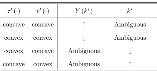
Table 1: Main Results of Section 4.2

0_{( ) v}0_{( ) Y(k ) k}

concave concave " Ambiguous

convex convex # Ambiguous

convex concave Ambiguous #

concave convex Ambiguous "

rate. In this case, a high-wage earner will be more reluctant to increase his labour supply as $

increases. The inequality in (27) is now reversed which meansn($) is a concave function. When

comparing across consumers with di¤erent rate of time preference, it su¢ce to note that the

after-tax wage rate in (26) is linearly increasing in :Thus, an increasing concave v0_{( ) will imply that}

n(k; ; ") is increasing and convex in :A mean-preserving spread in then leads to an increase in

the average value of "n(k; ; ") across all types of consumers, i.e., N(k) Ne(k) for all plausible

value of k:

The above arguments can be (partially) extended to allow for corner solutions in n: Let_bn($)

be the solution of the unconstrained problem, i.e.,v0_{[nb($)] =$for all$:Ifbn($)is convex, then}

the composite function maxf_bn($);0g is also convex but minf_bn($);1g is not. Thus, the …rst

part of Proposition 8 is valid so long as the optimal labour supply is strictly less than one. This

can be ensured by imposing the condition v0_{(1) > w(k}

max)": Likewise, if nb($) is concave, then

minfbn($);1g is also a concave function but maxfnb($);0g is not. Thus, we have included the

condition lim

n!0v

0_{(n) = 0 in the second part of Proposition 8 to ensure thatn >0:}

Based on the shape of 0_{( ) and v}0_{( ); we can identify four possible scenarios. Table 1}

sum-marises the overall e¤ects of greater time preference heterogeneity in each of these cases. These

can be easily seen with the aid of Figure 1a, hence the proof is omitted. For instance, when both

0_{( )andv}0_{( )are concave, an increase in time preference heterogeneity will shift both the national}

income function and the aggregate labour supply function up, according to Propositions 5 and 8.

This will lead to an unambiguous increase in national income, but an ambiguous e¤ect on the

capital-labour ratio. The latter is the result of two opposing forces: on one hand, an increase

in time preference heterogeneity will lower the average marginal tax rate on asset return which

encourages capital accumulation; on the other hand, such an increase will lead to an expansion

quantitative question. The other three cases in Table 1 can be interpreted in a similar fashion.

4.3 Numerical Examples

In the previous two sections, we have identi…ed two channels through which greater time

pref-erence heterogeneity can a¤ect the economy. The …rst one involves changing the cross-sectional

distribution of marginal tax rates and the national income function, while the second one involves

a composition e¤ect on aggregate labour supply. In this section, we will use numerical examples to

demonstrate these e¤ects in the full version of the baseline model. There are two reasons why we

resort to quantitative analysis here. Firstly, the presence of income e¤ect on labour supply poses a

serious challenge in characterising the shape ofn(k; ; ") as a function of :As a result, we cannot

ascertain qualitatively the e¤ects of greater time preference heterogeneity on N( ) as in

Proposi-tion 8. Secondly, as Table 1 suggests, the overall e¤ects of greater time preference heterogeneity

are often qualitatively ambiguous:The numerical examples presented below are intended to throw

some light on these issues.

Consider a parameterised version of the baseline model with the following speci…cs: One period

in the model is a year. The consumer’s period utility function is given by

U(c; n) = lnc A n

1+1=

1 + 1= ;

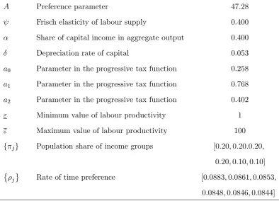
whereA is a positive-valued parameter and is the Frisch elasticity of labour supply. The value

of A is calibrated so that, on average, consumers spend about one-third of their time working in

the steady state. The resulting value ofA is 47.28. The Frisch elasticity of labour supply is set to

0:40;based on the estimates by MaCurdy (1981) and Altonji (1986). The production function is

assumed to take the Cobb-Douglas form, i.e.,F(K; N) =K N1 ;with = 0:40:We choose the

value of so that the steady-state capital-output ratio matches the value observed in the United

States over the period 1947-2016, which is 2.367.29 _{The required value of is5:3%:The progressive}

tax function is assumed to take the form in (24), with a0 = 0:258 and a1 = 0:768as reported by

Gouveia and Strauss (1994).30 The value of a2 is determined in two steps: First, we assume that

government spendingGaccounts for 20.7% of aggregate outputF(K; N)in the steady state. This

value is based on the share of government consumption expenditures in US GDP over the period

2 9_{We use the sum of private …xed assets and end-of-year stock of private inventories as our measure of aggregate}

capital stock. Data on private …xed assets and private inventories are obtained from the National Income and Product Accounts (NIPA).

3 0_{The same value ofa}

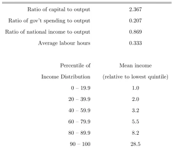
Table 2 Targeted Statistics

Ratio of capital to output 2.367

Ratio of gov’t spending to output 0.207

Ratio of national income to output 0.869

Average labour hours 0.333

Percentile of Mean income

Income Distribution (relative to lowest quintile)

0 – 19.9 1.0

20 – 39.9 2.0

40 – 59.9 3.2

60 – 79.9 5.5

80 – 89.9 8.2

90 – 100 28.5

1947-2016. We then solve the government’s budget constraint in (8) fora2:

In terms of consumer characteristics, we assume that labour productivity is uniformly

dis-tributed across consumers with " = 1 and "= 100: The distribution of ; on the other hand, is

calibrated so that the distribution of pre-tax income in the benchmark numerical example matches

certain features of its real-world counterpart.31 Speci…cally, we divide the entire population into

M income groups. All consumers within group j have the same level of pre-tax income y_j; for

j 2 f1;2; :::; Mg:These incomes are ranked according to y₁ < ::: < y_M: The population share of

income groupjis denoted by j 2(0;1);withPMj=1 j = 1:Since there is an one-to-one mapping

between pre-tax income and rate of time preference, all members within the same income group

have the same which can be determined by y_j = y k ; _j ; for all j: To construct a realistic

income distribution, we …rst compute the relative income$j yj=y1 for six income groups based

on the 2016 Survey of Consumer Finance (SCF) data reported in Bricker et al. (2017) Table 1.32

These income groups include the bottom four quintiles, the 80-89.9 percentile and the top 10% of

3 1_{Since the pre-tax income functiony(k; )is independent of";the cross-sectional distribution of labour}

produc-tivity is irrelevant here.

3 2_{Speci…cally, we use the mean income data in 2016 to compute the relative incomes f$}

jgM_j=1: We have also

Table 3 Benchmark Parameter Values

A Preference parameter 47.28

Frisch elasticity of labour supply 0.400

Share of capital income in aggregate output 0.400

Depreciation rate of capital 0.053

a0 Parameter in the progressive tax function 0.258

a1 Parameter in the progressive tax function 0.768

a2 Parameter in the progressive tax function 0.402

" Minimum value of labour productivity 1

" Maximum value of labour productivity 100

f jg Population share of income groups [0:20;0:20:0:20;

0:20;0:10;0:10]

j Rate of time preference [0:0883;0:0861;0:0853;

0:0848;0:0846;0:0844]

Table 4 Results of Numerical Examples

Benchmark % Changes from Benchmark

= 0 = 0:05 = 0:10 = 0:20 = 0:10

k 4.204 0.02% 0.05% 0.09% -0.04%

N(k ) 19.475 -0.37% -0.64% -1.00% 1.57%

Y (k ) 30.058 -0.37% -0.62% -0.97% 1.55%

k N(k ) 81.873 -0.35% -0.59% -0.91% 1.53%

(k ) N(k ) 34.589 -0.36% -0.62% -0.97% 1.55%

Capital-Labour Ratio

4.2 4.21 4.22 4.23 4.24 4.25 4.26 4.27 4.28 4.29

N a ti o n a l In c o m e 0 10 20 30 40 50 60 70 80 90 100

National Income Function

Capital-Labour Ratio

4.2 4.21 4.22 4.23 4.24 4.25 4.26 4.27 4.28 4.29

A g g re g a te L a b o u r S u p p ly 17 18 19 20 21 22 23 24 25 26 27

Aggregate Labour Supply Function

theta = 0 (Benchmark)

theta = 0.10

theta = 0.20

theta = -0.10

Figure 2

the income distribution.33 We then compute the value ofy₁ so that the ratio of national income

Y (k) to aggregate output F(K; N) is 0.869 in the steady state. This matches the value

ob-served in US data over the period 1947-2016.34 Once y₁ is known, we can solve for _j M_j=1 using

y_j = $jy1 =y k ; j ;for all j: Table 2 summarises all the targeted statistics mentioned above

and Table 3 shows the benchmark parameter values. The resulting value of six key variables,

namely the capital-labour ratiok ;aggregate labour inputN(k );national income Y(k );

aggre-gate capital k N(k );aggregate output(k ) N(k )and government spending G , are reported

in Table 4.35

The next step is to construct some alternative distributions of with di¤erent degrees of time

preference heterogeneity. Intuitively, a mean-preserving spread of the benchmark distribution can

be obtained by “hollowing out” the middle section and relocating the mass to the upper and lower

3 3_{Hence, we setM= 6;}

j= 0:20forj2 f1; :::;4gand 5= 6= 0:10:

3 4_{We use net national product as our measure of national income in this calculation. Data on net national product}

are obtained from the NIPA.

ends. To put this in practice, …rst choose a value from the range [0; 3]:Then de…ne a new set

of weights fejg on j as follows: e3 = 3 ; e1 = 1+ ; e6 = 6+ ;and ej = j for

j2 f2;4;5g:The value of is chosen so that the mean value of is unchanged, i.e.,

6

X

j=1

ej j =

6

X

j=1

j j:

Using this procedure, we construct four alternative distributions of with 2 f0:05;0:10;0:20; 0:10g:

We then solve the baseline model under each of these distributions, while keeping all other

pa-rameters in Table 3 unchanged. In general, a larger value of represents a higher level of time

preference heterogeneity. Thus, the distribution with = 0:10 is actually less diverse than the

benchmark distribution.

Figure 2 shows the national income function and aggregate labour supply function obtained

under various values of , including the benchmark case( = 0).36 _{Two results are immediate from}

these diagrams. Firstly, increasing the cross-sectional dispersion of causes the national income

function to shift upward. This pattern is consistent with the theoretical predictions in Proposition

5. Secondly, an increase in time preference heterogeneity will cause the aggregate labour supply

function to shift down. In a robustness check, we …nd the same pattern under di¤erent values of

within the range of [0;1]:37 Thus, at least in this regard, the calibrated model behaves similarly

as the “no-income-e¤ect” model considered in Section 4.2 with a convexv0( ):The key variables

obtained under these alternative distributions are shown in Table 4. Overall, these results suggest

that increasing the cross-sectional dispersion in consumer’s time preference has only a mild positive

e¤ect onk ;but a more signi…cant and negative impact on aggregate labour supply. The changes

in other aggregate variables are largely driven by the changes inN(k ):We can further divide the

e¤ects on N(k ) into (i) a composition e¤ect brought by the changes in the composition of the

workforce [i.e., changes inf 1; :::; 6g], and (ii) a general equilibrium e¤ect brought by the changes

in k (which a¤ect the level of individual labour supply). The contribution of these two e¤ects

are shown in Table 5. These results show that the negative impact of greater time preference on

N(k ) is due to a dominating composition e¤ect.38

3 6_{The curves for = 0:05are almost indiscernible from those obtained from the benchmark case, hence they are}

omitted from these diagrams.

3 7_{These results are not shown here due to space constraint. They are reported in the working paper version}

available on the authors’ personal website.

3 8_{We have also repeated the numerical exercise under a revenue-equivalent restriction. Speci…cally, for each}

alternative distribution of ;the value ofa2is re-calibrated so that (i) the government budget constraint is satis…ed;

Table 5 Two E¤ects on Aggregate Labour Supply

% Changes from Benchmark

= 0:05 = 0:10 = 0:20 = 0:10

Composition e¤ect -1.46% -2.92% -5.83% 2.92%

G.E. e¤ect 0.94% 1.78% 3.22% -2.53%

5

Conclusion

In this paper we analyse the long-run economic e¤ects of diversity in a deterministic neoclassical

model with ex ante heterogeneous consumers, ‡exible labour supply and progressive taxation.

Our results highlight two important channels through which consumer heterogeneity can a¤ect the

steady state. Firstly, changing either the distribution of labour productivity or time preference will

a¤ect the composition of aggregate labour supply. The exact nature of this e¤ect is determined

by the shape of the individual labour supply function. Secondly, changing the distribution of time

preference will also have an impact on the cross-sectional distribution of marginal tax rate. We

show that the curvature of the marginal tax function holds the key in determining this e¤ect. In

this analysis, we assume that time preference and labour productivity are independent of each

other. This assumption is adopted mainly for analytical convenience. As pointed out by Carroll

and Young (2009), such a model may fail to capture the observed patterns of correlation between

di¤erent types of income. One possible direction of future research is to analyse the e¤ects of

diversity without imposing the independence assumption. The model considered here also does

not take into account the political institutions that contribute to the progressive tax system or

other redistributive policies. As discussed in Alesina and La Ferrara (2005), these institutions play

a crucial role in resolving the con‡icting interests within a diverse population, and this will in

turn determine the economic e¤ects of diversity. One exciting and important direction of future

research is to introduce some political elements (such as a voting mechanism) into our baseline

model and analyse the e¤ects of diversity in a politico-economic equilibrium.

Appendix

Proof of Lemma 1

De…ne (k) f(k) kover the interval[kmin; kmax]:Then equation (14) can be more succinctly

expressed as Y(k) = (k)N(k): We will examine the properties of each of these functions,

starting with ( ): Since f( ) is strictly increasing and strictly concave, there exists a unique

valuekGR >0 such that 0(k)?0if and only ifk7kGR:Since 0(kmax) =f0(kmax) = >0;

we have kmax < kGR which means ( ) is strictly increasing over [kmin; kmax] with (kmin) >0:

Next, consider the national income functionY ( ):Since ( ) is strictly increasing,Y ( )is strictly

decreasing on (kmin; kmax) with

Y (kmax) =

Z

1 dH1( )>0;

and

lim

k!kminY (k) =

Z

1 (1 ) dH1( ): (28)

Equation (28) follows from the facts that ( ) is a continuous function and r(k) approaches

=(1 ) asktends to kmin:Note that the limiting condition lim

y!1

0_{(y) = implies}

lim

! 1 (1 ) = +1:

Hence, the integral in (28) can be either convergent or divergent. For instance, if H1( ) has a

positive mass at ;thenY (kmin) is in…nitely large and (17) is automatically satis…ed.

Finally, we will show that the aggregate labour supply function N( ) is non-decreasing. It

su¢ce to show that n(k; ; ") is non-decreasing in k; for all ( ; "): Fix ( ; ") and suppose the

contrary that 1 n(k2; ; ") > n(k1; ; ") 0 for some k1 > k2 in [kmin; kmax]: Since c(k; ) is

strictly decreasing ink, we have c(k1; )< c(k2; ):By Assumption A2, (c; n) is non-decreasing

incand strictly increasing in n: Hence, we have

w(k1)

r(k1)

" [c(k1; ); n(k1; ; ")]

< [c(k2; ); n(k2; ; ")]

w(k2)

r(k2)

" < w(k1) r(k1)

" :

andr( ) is strictly decreasing. Since there is a contradiction,n(k; ; ")must be non-decreasing in

kfor all possible values of ( ; "):

The above results implies that [Y (k) (k)N(k)] is strictly decreasing over the interval

(kmin; kmax): If (16) and (17) are satis…ed, then there exists a unique value k within this range

that solves (14). Conversely, if this equation has a unique interior solution, then the two curves

in Figure 1a must cross once over the interval (kmin; kmax), which implies (16) and (17). This

completes the proof of Lemma 1.

Proof of Lemma 2

Fixk2(kmin; kmax)and 2 ; :Suppose the contrary that1 n(k; ; "2)> n(k; ; "1) 0 for

some"1 > "2 in["; "]:Since (c; n)is strictly increasing in n, we have

w(k)

r(k) "1 [c(k; ); n(k; ; "1)]< [c(k; ); n(k; ; "2)]

w(k)

r(k) "2

< w(k)

r(k) "1;

which is a contradiction. Hence, n(k; ; ") must be non-decreasing in ":If n(k; ; ") is an interior

solution, then it is completely characterised by

[c(k; ); n(k; ; ")] = w(k)

r(k) ":

By Assumptions A1-A2 and the implicit function theorem,n(k; ; ") is continuously di¤erentiable

in". Straightforward di¤erentiation then yields

@ @n

@n(k; ; ")

@" =

w(k)

r(k) >0:

Since @ =@n >0;the desired result follows. This completes the proof of Lemma 2.

Proof of Proposition 3

We …rst establish an intermediate result.39

3 9_{The proof of Lemma A1 has been outlined in Shaked and Shanthikumar (2007, p.204-205). We include a more}