Munich Personal RePEc Archive
A note on the relation between fiscal
equalization and economic growth
Chan, Felix and Petchey, Jeff
Curtin University
15 May 2017
Online at
https://mpra.ub.uni-muenchen.de/79156/
A note on the relation between fiscal equalization
and economic growth
Felix Chan, Jeff Petchey
∗Department of Economics, Curtin University, Perth, WA, Australia
May 15, 2017
1 Introduction
The objective of fiscal equalization, which is implemented in many federal and decen-tralized unitary countries1 is to give sub-national regions (e.g. states, provinces or local governments) comparable capacities to provide local public services without imposing different tax burdens on their populations. The representative tax system, or RTS, is the standard approach used to achieve equalization. It usually is embedded within a broader tax revenue sharing structure established between central and regional govern-ments. Under the RTS approach a region is compensated through transfers from the centre for any difference between the revenue raised when average regional tax rates are applied to its tax bases and the revenue raised when average tax rates are applied to the tax bases of all regions. This difference is positive for low income regions - they have a positive revenue need - and it is negative for relatively high income regions who are assessed to have a negative revenue need.
Equalization schemes are, therefore, implicitly redistributive between regions. In-deed, this is necessary in order to achieve their (equity) objective of ensuring sub-national regions have comparable fiscal capacities.
∗Email: [email protected] or [email protected]. 1
Weingast (2009) has argued that the inter-regional redistribution arising from equal-ization creates disincentives for regions to develop their economies over time and that this adversely affects economic growth. He illustrates the idea with an example based on the “fiscal law of 1/n” that supposes there aren provinces with the average province receiving 1/nof some total revenue pool regardless of its own policies. Weingast (2009) then supposes a province adopts growth enhancing policies which increase its revenue base and argues that “... the province receives 1/n of the total increase in revenue generated solely from its increased investment in the local economy. The province bears the full expenses for the market-enhancing public goods but captures only 1/n
of the fiscal return.”2 He also notes that: “... fiscal systems that allow growing regions to capture a major portion of new revenue generated by economic growth provide far stronger incentives for local governments to foster local economic growth.”3
This raises an important question, namely, could the redistribution arising from fiscal equalization in practice have adverse consequences for the rate of growth in total output over time? The economics literature on this question is sketchy. Some research has examined the impact of federalism and decentralization, though not equalization, on inter-temporal per capita income. We refer here, for example, to Zhang and Zou (1999), Xie et al. (1999), Akai and Sakata (2002), Brueckner (2006) and Thornton (2007). As far as we are aware, only Ogawa and Yakita (2009) and Cyrenne and Pandy (2013) have examined the relationship between equalization and inter-temporal per capita income. However, Ogawa and Yakita (2009) focus on equalization and the convergence of regional economies while Cyrenne and Pandy (2013) examine equaliza-tion and the composiequaliza-tion of government spending. This leads us to agree with the point made by Fischer and Ulrich (2011) that “... the existing theoretical....growth literature that incorporates vertical or horizontal transfers across government tiers is scant.”4
The contribution of this note is to shed some light on this question. We do this by first presenting a case study of the inter-regional redistribution induced by fiscal equalization in Australia. This country is chosen because, as will be explained in the paper, it has the most comprehensive of all equalization systems and serves to
2
Weingast (2009) pages 283 and 284. See also Careaga and Weingast (2003) for an analysis of the law of 1/nas it applies to redistributive policies generally.
3
Weingast (2009) page 284.
4
highlight the empirical magnitude of the inter-regional redistribution that can arise from equalization of fiscal capacities. This degree of redistribution will be replicated, to varying degress, in any country with equalization across its regions. The case study therefore provides some context to the paper and its results by showing how important the transfers induced by equalization can be in practice.
We then construct an economic model with regions linked through an RTS equal-ization scheme. Regional economies are also subject to economic growth dynamics. Each region is assumed to maximize its inter-temporal social welfare over a fixed time horizon by choosing an optimal saving rate. This will then determine capital accumu-lation, investment and output over the same period. The choice of a fixed time horizon is justified by two practical considerations. Firstly, saving rates cannot be changed instantaneously in practice and are often chosen for a fixed period of time. Secondly, the regional government itself may change over time depending on the outcome of re-gional elections which usually occur at regular intervals. It is assumed that when a new regional government takes office, it will determine its main policies for the duration of its term, including its savings and capital accumulation plans. In this sense our fixed term horizon may correspond to an election cycle.
comparable to what we attempt to achieve.
With this in mind, our main contribution is to show that RTS-type fiscal equal-ization provides incentives for regions to reduce saving rates below what they would choose in the absence of equalization. Since regional capital accumulation and per capita output are increasing in savings rates, this also means that capital spending and per capita output are lower over time than otherwise. It is also the case that the growth rate in total output is lower when regions are subject to equalization. We conclude, therefore, that when considered in an inter-temporal context, equalization may reduce incentives for regions to develop their economies, as suggested by Weingast (2009).
We qualify this finding and put it into further context in the Conclusion. There it is argued that any inter-temporal growth costs of equalizaton, such as identified in this note, must be weighed against the possibile benefits of equalization, which may be considerable. They arise from inter-regional equity considerations and the possible efficiency gains related to factor mobility identified elswhere in the fiscal federalism and public economics literatures over a substantial period of time (see Conclusion).
The note is organized as follows. Section 2 presents the case study. Section 3 develops a model of an inter-temporal economy with regions and RTS-type fical equal-isation. In Section 4, we analyse a policy game between regions in which they choose their savings rates to maximize regional social welfare. This section also presents the results while Section 5 concludes. Most technical details are relegated to appendices.
2 Case Study: Equalization in practice
Australia has eight states subject to centrally mandated fiscal equalization.5 The country is considered to have the most comprehensive fiscal equalisation scheme in the world for two main reasons. First, the Australian approach raises all states to the fiscal capacity of the strongest rather than the average. Hence, the redistributive task required by the Australian approach in order to achieve equalization is large. Second, it measures all revenue and expenditure needs thus making it a technically demanding and detailed approach which is seen as a benchmark in the practice of equalization.
5
These features make the Australian model of particular interest as a case study to provide context for our theoretical results. Elements of the Australian model are to be found in all equalization schemes adopoted world-wide.
To be more specific, the Australian scheme applies the principles of equalization in allocating the Goods and Services Tax (GST) revenue pool to the states.6 In 2015-16, the GST pool was approximately $57.2 billion. The Australian model breaks equalisa-tion down into three steps. In the first, states with relatively low fiscal capacities, the Northern Territory, Tasmania, South Australia and Queensland, are raised to the av-erage fiscal capacity of all states. This ensures that the States with relatively low fiscal capacities can provide the average standard of services without imposing a higher than averge tax burden on their citizens. In the second step, all states, except the fiscally strongest, are raised to the fiscal capacity of the strongest state, currently Western Australia.7 The final step sees any revenue left over in the GST pool after Steps 1 and 2 allocated to all states on an equal per capita basis.
After equalization, all Australian States have a fiscal capacity comparable to that of the fiscally strongest state, Western Australia. During the financial year 2015-16, 12% of the GST pool, or $6.8 billion, was used for the first step, and 58%, or $33.2 billion, for the second step. Hence, achieving the total equalization task consumed 70% of the GST pool or $40.0 billion in 2015-16. This equates to about 2.4% of Australia’s GDP. The remaining 30% of the GST pool, or $12.2 billion, was allocated to the states on an equal per capita basis.8 The GST pool in Australia is more than sufficient to bring all states up to the fiscal capacity of the strongest state. This is unlike some other countries that adopt equalization in some form, for example China, where the pool of revenue available for distribution from the national government is insufficient to achieve such a comprehensive degree of equalization (see Wang and Herd (2013)).
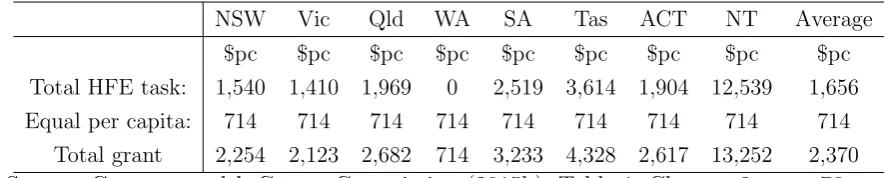
To illustrate further, the per capita amounts allocated to the Australian states for Steps 1 and 2 combined (the total equalization task), and Step 3 (the equal per capita part of the allocation), are illustrated in Table 1 for the financial year 2015-16. Since it is the fiscally strongest, Western Australia received nothing from the GST pool to complete the total equalization task (Row 1) while the other states received positive
6
See Commonwealth Grants Commission (2015b) for detailed discussion.
7
Historically, this been either Victoria or New South Wales. However, as a result of a resources boom, this position is now occuppied by Western Australia.
8
per capita amounts, with the grant to each depending on its assessed fiscal capacity relative to the average for all States. Finally, all states received $714 per capita from Step 3, the equal per capita allocation.
Table 1: Allocation of the GST pool under equalization: The three steps, $pc, 2015-16
NSW Vic Qld WA SA Tas ACT NT Average $pc $pc $pc $pc $pc $pc $pc $pc $pc Total HFE task: 1,540 1,410 1,969 0 2,519 3,614 1,904 12,539 1,656 Equal per capita: 714 714 714 714 714 714 714 714 714
Total grant 2,254 2,123 2,682 714 3,233 4,328 2,617 13,252 2,370
Source: Commonwealth Grants Commission (2015b), Table 1, Chapter 3, page 76.
The final per capita grants from the GST pool are shown in the last row. They differ based on the relative fiscal capacities of the states before equalization. The Northern Territory received 18.56 times the per capita grant of Western Australia in order to raise its fiscal capacity to that of Western Australia. Tasmania and South Australia each received 5.06 and 3.52 times respectively the per capita grant of Western Australia.
It is clear from this discussion that equalization in Australia requires substantial redistribution between states, most notably from Western Australia but also New South Wales and Victoria, to the remaining states. The redistributive task is comparatively large because the Australian system brings all states up to the fiscal capacity of the strongest state. Though the Australian case may be an outlier in this particular sense, equalization will to some degree induce inter-regional redistribution in any economy that adopts it.9 Indeed, it must do so in order to achieve equalization of fiscal capacities across economically disparate regions.
The question we now address in the next Sections of the note is whether the redis-tribution we observe in this case study has the potential, at least in theory, to affect savings, capital accumulation and growth in total output over time.
9
3 An inter-temporal regional economy with equalization
In this Section, we develop a model of an inter-temporal regional economy, which can be thought of as a federation, a regional union of nation-states or a unitary country with local jurisdictions. The economy is assumed to have two regions, j = 1,2. It is also assumed there is a centrally mandated RTS-style equalization scheme in place that redistributes from high to low income regions. LetYj(t),Kj(t),Lj(t) andAj(t) denote
the output, capital stock, labour and technology of region j at time t, respectively. The change in capital stock in regionj is assumed to follow
Kj,t(t) =sjYj(t)−θjKj(t) (3.1)
where Kj,t(t) is the time derivative of Kj(t) with sj and θj denote the saving and
depreciation rates, respectively. The model also assumes a citizen supplies a fixed unit of labour soLj(t) is also the population of regionj. We also assume both labour supply
and knowledge grow at constant rates with the following dynamics,
Lj,t=(1 +nj)Lj(t) (3.2)
Aj,t=(1 +gj)Aj(t), (3.3)
and output of region j is given by Yj(t) = Yj(Aj(t), Lj(t), Kj(t)). These specification
are consistent with the Solow-Swan growth model. For more details, see, for example, Romer (2001). In the Solow-Swan model, however, the saving rate, sj, is exogenous.
In our model, we make the savings rate in each region a choice variable chosen by the region’s goverrment to maximise its social welfare over a fixed horizon,t= 0, ...., T.
This is justified supposing that the total saving rate for a region’s economy, sj,
is a combination of its public and private savings rates. Thus, the role of a regional government is to determine its separate public savings rate conditional on some given, and constant, private saving rate. Further, regions are assumed to make this choice such that the total savings rate in their region is consistent withsj. It is this assumed
Having developed the dynamics of the regional economy we now introduce and embed the RTS-type equalisation rule. The formal derivation of this policy rule can be found in Appendix A. The basic idea is that the central government appropriates some portion of the per capita output of region j at a given rate which is the same across regions. The revenue collected by the centre (for example, this could be the GST pool in Australia) is then redistributed to the regions using lump-sum unconditional grants that equalize for revenue needs consistent with the RTS approach based on different revenue needs. Hence, each region makes a per capita contribution to the central revenue pool and receives a grant from it, with its net transfer, denoted asρj,
equal to the difference between the two. As shown in Appendix A, the net transfer under the assumed RTS scheme can be expressed as
ρj(t) =
1− Yj(t)
Lj(t)
L(t)
Y(t)
Q(t)
L(t), (3.4) where Y(t) = Y1(t) +Y2(t) is the total national outputs, L(t) = L1(t) +L2(t) is the total national population and Q(t) is the total national expenditure on public goods. As will be shown below, this introduces strategic opportunities for regions since they can manipulate the net transfers through the choice of saving rates. Distortions arising from this strategic behaviour over net transfers are the prime interest in this paper.
When regions are asymmetric, as when they have different production technologies, the contribution of a particular region to the pool relative to what it gets back by way of an equalization grant will be different. This is because they will each make divergent per capita contributions to the pool and receive different equalization grants based on the RTS approach. For these reasons, the net transfer received by a region will be positive or negative. What is more, as shown in Appendix A the net transfer received by regionj must have the opposite sign to the net transfer received by region
i where i = 1,2 and i 6= j. The sum of the net transfers must also be equal to zero. Furthermore, a relatively low income region will have a positive net transfer, adding to its locally produced output, while a comparatively high income region will have a negative net transfer, detracting from its produced output.
national public goods or undertake any other form of redistribution.
Moreover, the centre does not implement an optimal equalization rule derived from maximizing national social welfare. Rather, the equalization policy rule is given and based on the real-world RTS scheme that we see in practice. These choices are delib-erate simplifications which allow us to focus on how regional behaviour is affected by an RTS-type equalization policy rule in an inter-temporal context.
Given this set up, we now complete the model specification by describing how income for citizens in each region is determined. We also develop an inter-temporal social welfare function for each region that takes account of regional economic dynamics and equalization. This provides a basis for the regional optimization problem in the next Section and the results presented and discussed there.
Income available in each region for conversion into public goods and consumption, denotedπj forj = 1,2, is the sum of produced output less saving and the net transfer,
ρj, described above. The budget constraint of region j at a particular point in time is
therefore
xj(t) +cjqj(t) = (1−sj)Yj(t) +Lj(t)ρj(t) (3.5)
wherexj(t) and qj(t) denotes private and public goods, respectively, with cj represents
the relative price of public goods to private good. In other words, the price of private goods is being normalised to one.
Let uj[xj(t), qj(t)] denotes the utility function of a representative citizen in region
j. Regions are assumed to provide local public goods consistent with a first-best rule. In other words, the local public goods provided by region j, q∗
j(t), along with the
local private goods, x∗
j(t), maximise the utility function, uj(t), subject to the budget
constraint as stated in equation (3.5). Expressions for the provision of local public goods consistent with this are provided in Appendix B. The indirect utility function for regionj can then be obtained by
Vj(t) = uj
x∗
j(t), q∗j(t)
. (3.6)
Social welfare in region j is defined as the weighted sum of indirect utility of a representative citizen:
Wj(t) = Z T
0
wheret= 0, ..., T is some fixed horizon. Since regional governments are assumed to be benevolent, making their choice of saving rate to maximize social welfare within their own region, equation (3.6) also defines the objective function for the government of regionj wherej = 1,2. That is, regionj chooses sj to maximize inter-temporal social
welfare consistent with the growth dynamics and net inter-regional transfer incorpo-rated into equation (3.6).
This completes the specification of the inter-temporal regional economy with equal-ization. The next Section develops a policy game between regions and presents results.
4 Policy game and results
From the discussion above, the net transfer received by a region is a function of out-puts from both regions implying that equalization creates interdependence between the policy choices made by regions. We now capture this in a game where regions choose their saving rates as Nash competitors. This means each region chooses its saving rate for a given choice in the other region. In this game, regions are assumed to correctly anticipate the impact of their saving rate choices onρj(t), their net transfer.
By solving the resulting maximization problem of each region we are able to obtain first order necessary conditions or best response functions for each region. Under Nash conjecture, we can consider this policy game as simultaneous. With full information each region chooses its optimal strategy according to its best response.
The maximization problem for region j with equalization is
max
sj
Wj(t) (4.1)
whereWj(t) is defined in equation (3.7). As noted above,Wj(t) defines social welfare
in region j under the economic dynamics and equalization rule described in Section 3 and in detail in Appendix A. Under our behavioural assumptions, region j takes account of the impact of its choice of sj on its contribution to the central pool, its
equalization grant and its produced output over the fixed horizont = 0, . . . , T. To be specific, regionj acts strategically with respect to the equalization policy rule.
Proposition 1. The net transfer is a decreasing function of saving rate. Specifically,
ρj,s(t)<0.
Proof. See Appendix C.
This tells us that if region j increases saving rate, it decreases its per capita net transfer. As shown in the proof, this holds without restriction for both regions regard-less of their relative outputs. It means that region j can increase its net transfer by reducing its saving rate which leads to lower output. Now consider the next proposition:
Proposition 2. The optimal saving rate in region j, s∗
j, satisfies
RT
0 exp (−δt)uj,xjLjρj,s(t)dt+ RT
0 exp (−δt)uj,xjYj(t)dt
=RT
0 exp (−δt)uj,xj(1−sj)Yj,sdt
(4.2)
for j = 1,2.
Proof. See Appendix C
The first order condition for sj characterizes two best response functions, ˆs1 = ˆ
s1(s2) and ˆs2 = ˆs2(s1), between the strategy of a region and that of its neighbour. A Nash equilibrium to the policy game is, therefore, a solution, s∗ = (s∗
1, s∗2), such that
s∗
1 = ˆs1(s∗2), s∗2 = ˆs2(s∗1).
The first term on the left side is the change in the net transfer to region j resulting from an incremental increase in sj per unit of income. From Proposition 1, ρj,sj <0,
forj = 1,2, so the region will consider this to be a marginal cost from an incremental increase insj. The second term on the left side captures the change in produced output
available for public and private good consumption arising from an increase in sj. An
increase in the saving rate means that the proportion of produced output available to consume public and private goods at time t is smaller. Therefore, the region will also consider this to be a marginal cost of an increase in its savings rate. The term on the right side of equation (4.2) captures the effect of an incremental increase in the saving rate on output. This is a marginal benefit of increasing the saving rate since it increases capital accumulation and hence output.
In summary, the left side of the first order necessary condition for sj captures
equalization cost in terms of lost net transfer and a cost arising from lower output at timet. The right hand side captures the marginal benefit of increasing the saving rate in terms of a marginal increase in regional output because of higher capital accumulation. In choosing its optimal saving rate region j equates the sum of these two marginal costs with the single marginal benefit.
Now consider the scenario where there is no fiscal equalization policy rule and
ρj(t) = 0 for all j and t. In this scenario the regions are two separate economies and
regional decision makers have dominant strategies with regard to their choice of saving rate. It is straight forward to show that the first order condition for sj becomes
Z T
0
exp (−δt)uj,xjYj(t)dt= Z T
0
exp (−δt)uj,xj(1−sj)Yj,sdt (4.3)
for j = 1,2. An equilibrium is a solution, s0
j, that solves equation (4.3) for j = 1,2.
The left side is the change in produced output available for public and private good consumption arising from an increase in sj. The region will consider this to be a
marginal cost of a higher saving rate. The right side is the marginal benefit of an incremental increase in the saving rate in terms of capital accumulation and output. The region considers this to be a marginal benefit of increasing its savings rate. As with the scenario with the equalization plicy rule in place, regions choose their saving rate to equate marginal cost and benefit.
By comparing equations (4.2) and (4.3), one can see equalization introduces an ad-ditional marginal cost of an increase insj, namely,
RT
0 exp (−δt)uj,xjLjρj,s(t)dt, without
any corresponding marginal benefit. This allows us to conclude with the following
Proposition 3. Equalization induces regions to under-save relative to the case where there is no equalization policy rule.
Proof. From equations (4.2) and (4.3) above,s∗
j < s0j, for j = 1,2.
Since capital accumulation and per capita output are increasing sj it follows that
leads to a lower growth rate in total output than the scenario with no equalization.10
5 Conclusion
We conclude by noting that these theoretical results should not necessarily be taken to imply that countries are unwise on economic grounds to equalize their sub-national regions using RTS-type schemes. This is because equalization may achieve important inter-regional equity, political, national citizenship or other objectives not captured in our model. Moreover, as highlighted in the fiscal federalism literature, the transfers induced by equalization may be efficiency enhancing if there are fiscal externalities associated with inter-regional migration and/or if regions collect economic rents and disburse them on the basis of residency. This has been shown using static models of regional economies as in, for example, Boadway and Flatters (1982), Myers (1990), Caplan et al. (2000) and Boadway et al. (2003). Since we assume in our model above that factors of production are immobile we do not allow for the possibility that transfers can also, potentially, result in spatial efficiency gains. Future extensions of our model may allow for factor mobility so that the distortions to savings and capital accumulation we capture can be considered within this wider context.
Nevertheless, for now the results in this note at least suggest that if equalization is implemented to support these other objectives it may have inter-temporal costs in terms of distortions to regional savings, capital accumulation and the growth rate in total output. This potential inter-temporal cost of equalization has not been empha-sised previously in the literature yet may be important to consider in theoretical and policy debates over the general benefits and costs of fiscal equalization in decentralized economies, such as federations.
10
Appendix A: Equalization policy rule
The specific equalization rule we consider is a stylized variant of the Australian model which, as noted in the main text, is an application of an RTS-type approach. Under this model, the grant received by a region, which we will calls states for the purposes of this Appendix, has two components; a revenue sharing equal per capita grant and an equalization grant based on revenue needs which is explicitly redistributive from high to low income states. It should be noted that as the Australian model is an application of the RTS approach our results do not depend on its adoption. It should also be noted that since the model below also incorporates an equal per capita grant to a state it is really a revenue sharing and equalization scheme, though for the purposes of brevity it is referred to simply as an equalization scheme.
Let us suppose a central government appropriates a portion of the output of state
j, at a rate 0< φ <1, which we assume to be a parameter independent of time. This appropriation captures the complex myriad of taxes used by central governments in practice to raise revenue. The per capita appropriation from the people of state j is,
τj(t) = φ
Yj(t)
Lj(t)
, j = 1,2. (A.1)
Total revenue collected from all citizens is
G(t) = φ
2
X
j=1
Yj(t) =
2
X
j=1
Lj(t)τj(t). (A.2)
In practice, central governments use the revenue they collect to provide services. Any surplus of revenue after the central government’s own activities - known as the fiscal gap - would be returned to the states as grants. We abstract from this com-plexity by supposing all centrally collected revenue is redistributed to the states as untied grants according to an revenue sharing-equalization formula.11 An implication is that the central government in our model provides no services. Its sole function is to appropriate revenue and create a revenue pool which is then distributed to the states. The discussion now focuses on each state separately, commencing with state 1. Let the per capita grant received by state 1 be defined as
g1(t) =
G(t)
L(t) +ξ(t) [1−ν1(t)] j = 1,2. (A.3)
11
Each component of the right hand side of the expression is explained below. 12
a. Revenue sharing component: The first term,G(t)/L(t), is an equal per capita share of the revenue pool allocated to all citizens of the country regardless of where they live. This can be thought of as the revenue sharing part of the grant received by a region. It is not explicitly redistributive, as is the equalization part of the grant expression, discussed in (b) to (d) below. However, it implicitly redistributes income across regions when per capita region incomes differ and each region makes the same per capita contribution to the central grant pool, as in our model.
b. Own-source revenue per capita: The second term. ξ(t), is the total per capita tax revenue raised by both states, which can also be thought of as an average state tax rate. It is defined as
ξ(t) = 1
L(t)[Q(t)−G(t)] j = 1,2. (A.4) In this expression, Q(t) is total state spending on local public goods, G(t) is the revenue pool previously defined andL(t) is total national population. It is assumed that total state spending exceeds the revenue pool, implying states raise positive own-source revenues; hence Q(t)−G(t) > 0 so ξ(t) > 0. Further, define total public good spending as
Q(t) = 2
X
j=1
cjqj(t) (A.5)
where qj(t) are quantities of local public goods provided by state j. The price of
the local public good in state 1, c1, is assumed to be a parameter, as is c2, the local public good price for state 2.
c. Revenue disability: Finally, ν1(t) is a measure of the strength of the tax base in state j relative to the total state tax base. We adopt per capita state output as a proxy for state tax bases. The disability is the ratio of per capita output in state 1 to per capita national output. This means:
ν1(t) =
Yj(t)
Lj(t)
L(t)
Y(t). (A.6) If per capita output in state 1 exceeds per capita national output, because state 1 has comparatively high per capita income, thenν1(t)>1. However, if per capita output
12
in state 1 is less than per capita national output, because state 1 has relatively low per capita income, then ν1(t)<1. From the construction of the revenue disability variable at equation (A.6), it follows that:
ν1(t)>1⇒ν2(t)<1
ν1(t)<1⇒ν2(t)>1.
(A.7)
The revenue disability for state 1 is also a function of the joint policy choices of the two states since Y(t) is an implicit function of s1 and s2, as by implication, is the analogous revenue disability for state 2.
d. Revenue need: Given the above definitions, the term ξ(t) [1−ν1(t)] in equation (A.3) is the revenue need of state 1, or the equalization component of the grant expression. In the event that ν1(t) > 1, then ξ(t) [1−ν1(t)] < 0 and the revenue need of state 1 is negative. From equation (A.3) this ensures the per capita grant to state 1 is below its revenue sharing entitlement. Ifν1(t)<1, thenξ(t) [1−ν1(t)]> 0, and state 1 has a positive revenue need. This ensures its actual per capita grant is above the per capita revenue sharing grant. Hence, the revenue need is the explicitly redistributive equalization component of the total grant to state j. It redistributes output from the rich to poor state by adding to, or subtracting from, a state’s revenue sharing component - the equal per capita part of the grant expression.
The degree of redistribution can be measured as a net transfer to each state which is positive or negative, depending on whether a state is poor or rich. Accordingly, we define the per capita net transfer to state 1 as
ρ1(t) =g1(t)−τ1(t). (A.8) There is also a balanced transfer constraint, L2(t)ρ2(t) = −L1(t)ρ1(t), which im-plies that the net transfer to state 2 is simply
ρ2(t) = −
L1(t)
L2(t)ρ1(t). (A.9) From this, the central grant pool is automatically exhausted by grants to the states and hence G(t) = L1(t)g1(t) +L2(t)g2(t) holds. This means there is no need for a separate balanced grant constraint in the maximization problem presented later.
Following from the construction above, it is possible to derive a more mathemati-cally conveniently expression for the net transfer. Specifimathemati-cally, by direct manipulation,
ρj(t) =
1− Yj(t)
Lj(t)
L(t)
Y(t)
Q(t)
L(t). (A.10)
Letuj(xj(t), qj(t)) be the utility function withxj(t) andqj(t) denote the total public
and private good consumptions in state j at timet. So the maximisation problem is max
xj(t),qj(t)
uj(xj(t), qj(t))
s.t. xj(t) +cjqj(t) = (1−sj)Yj(t) +Ljρj(t)
The Lagrangian function associated with this problem is
L=uj(xj(t), qj(t)) +λ[(1−sj)Yj(t) +Ljρj(t)−xj(t)−cjqj(t)]. (B.1)
The First Order Necessary Conditions are:
uj,xj −λ =0 (B.2) uj,qj+λ
Ljρj,qj−cj
=0 (B.3)
(1−sj)Yj +Ljρj −xj−cjqj =0 (B.4)
Note that FONC (B.4) implies that x∗
j,qj = Ljρj,qj −cj and λ∗ = uj,xj. Therefore
provision of local public goods in region j must satisfy
uj,qj +uj,xjx
∗
j,qj = 0.. (B.5)
Appendix C: Proof of Propositions
Proof of Proposition 1 : By direct calculation
ρj,s(t) =−
1− Yj(t)
Y(t)
Q(t)
Y(t)
Yj,s(t)
Lj(t)
.
Let
ξj(t) =−
1− Yj(t)
Y(t)
Q(t)
Y(t)Lj(t)
and note that ξ(t)<0 for all t. Moreover, Yj,s(t) = Yj,Kj(t)Kj,s, then ρj,s =ξ(t)Yj,KjKj,s.
Since Yj,Kj > 0 and Kj,s > 0 under the standard Solow-Swan assumptions, this gives
the result.
Proof of Proposition 2: The optimization problem is
max
sj Z T
0
where Vj(t) = uj(x∗(t), q∗(t)) is the indirect utility function. Then the first order
condition is
Z T
0
exp (−δt)Vj,s(t)dt= 0
where
Vj,s=λ∗(−Yj + (1−sj)Yj,s+Ljρj,s)
=uj,xj(−Yj + (1−sj)Yj,s+Ljρj,s)
by the Envelop Theorem. Therefore, the FONC is
Z T
0
exp (−δt)
uj,xj(−Yj + (1−sj)Yj,s+Ljρj,s)
dt= 0. (C.2)
By direct manipulation,
Z T
0
exp (−δt)
uj,xj(−Yj + (1−sj)Yj,s+Ljξ(t)Yj.s)
dt = 0. Z T
0
exp (−δt)
uj,xj
−Yj+
1−sj −
Y−j(t)
Y(t)
Q(t)
Y(t)
Yj,s
dt= 0
Z T
0
exp (−δt)uj,xj Y−j(t)
Y(t)
Q(t)
Y(t)Yj,sdt+
Z T
0
exp (−δt)uj,xjYj(t)dt
=
Z T
0
exp (−δt)uj,xj(1−sj)Yj,sdt.
REFERENCES
Akai, N. and Sakata, M. (2002). Fiscal decentralization contributes to economic growth: evidence from state level cross section data from the US. Journal of Urban Eco-nomics, 52:93–108.
Australian Government (2012). GST Distribution Review.Commonwealth of Australia, Canberra.
system of governance: a synthesis and extension of recent results. Canadian Journal of Economics, 44:82–104.
Brueckner, J. (2006). Fiscal federalism and economic growth. Journal of Public Eco-nomics, 90:2107–2120.
Caplan, A., Cornes, R., and Silva, E. (2000). Pure public goods and income redistri-bution in a federation with decentralized leadership and imperfect mobility. Journal of Public Economics, 77:265–284.
Careaga, M. and Weingast, B. (2003). Fiscal federalism, good governance, and eco-nomic growth in mexico. In Rodrik, D., editor, Search of Prosperity: Analytic Nar-ratives on Economic Growth. Princeton University Press, Princeton.
Commonwealth Grants Commission (2015a). Report on GST revenue sharing relativ-ities - 2015 update. Commonwealth of Australia, Canberra.
Commonwealth Grants Commission (2015b).Report on GST Revenue Sharing Relativ-ities, 2015 Review, Volume 1, Main Report. Commonwealth of Australia, Canberra. Cyrenne, P. and Pandy, M. (2013). Fiscal equalization, government expenditures and economic growth. Technical Report 2013:03, Department of Economics Working Paper, University of Winnipeg, Canada.
Evers, M. (2012). Federal fiscal transfer rules in monetary unions. European Economic Review, 56:5070–525.
Evers, M. (2015). Fiscal federalism and monetary unions: a quantitative assessment.
Journal of International Economics, 97:59–75.
Fischer, J. and Ulrich, T. (2011). Incentive effects of fiscal equalization: The case of france. Technical report, Munich Personal RePEc Archive.
Myers, G. (1990). Optimality, free mobility, and the regional authority in a federation.
Journal of Public Economics, 43:107–121.
Ogawa, H. and Yakita, S. (2009). Equalization transfers, fiscal decentralization, and economic growth. Finanzarchiv, 65:122–140.
Romer, D. (2001). Advanced Macroeconomics. McGraw-Hill Irwin.
Thornton, J. (2007). Fiscal decentralization and economic growth reconsidered.Journal of Public Economics, 61:64–70.
Weingast, B. (2009). Second generation fiscal federalism: The implications of fiscal incentives. Journal of Urban Economics, 65:279–293.
Xie, D., Davoodi, H., and Zou, H. (1999). Fiscal decentralization and economic growth in United States. Journal of Urban Economics, 45:228–239.