Practical Considerations for
Questionable IVs
Clarke, Damian and Matta, Benjamín
Universidad de Santiago de Chile, Universidad de Santiago de Chile
June 2017
Practical Considerations for Questionable IVs
Damian Clarke Department of Economics Universidad de Santiago de Chile
Benjam´ın Matta Department of Economics Universidad de Santiago de Chile
Abstract. This paper examines a number of techniques which allow for the construction of bounds estimates based on instrumental variables (IVs), even when the instruments are not valid. Theplausexog and imperfectivcommands are introduced, which implement methods described by Conley et al. (2012) and Nevo and Rosen (2012b) in Stata. The performance of these bounds under a range of circumstances is examined, leading to a number of practical results related to the informativeness of the bounds in different circumstances.
Keywords: IV, instrumental variables, exclusion restrictions, invalidity, plausibly exogenous, imperfect IVs
1
Introduction
Instrumental variables are a work horse estimator in economics as well as in other fields concerned with the causal estimation of relationships of interest. Nonetheless, credible instrumental variables (IVs) are hard to come by. While finding variables which are correlated with an endogenous variable of interest (“relevant” in IV terms) is generally not a challenge, motivating and defending a zero-correlation with unobserved error terms (“validity”) is much less straight-forward.1
As is well known, validity assumptions in an IV setting are untestable. While par-tial tests exist (Sargan 1958; Hansen 1982; Kitagawa 2015), these tests are necessary, rather than sufficient, to demonstrate instrumental validity. This often leads to the uncomfortable position where the best estimates for a parameter are based on a strong assumption, for which no definitive proof can be offered.
Given the importance of assumptions regarding the behaviour of unobservables in producing causal estimates in an IV setting, a range of methods have been proposed to preserve casual estimation with weaker assumptions. Work by Manski and Pepper (2000, 2009) loosened the validity assumption replacing strict equalities with (weak) inequalities. Extensions of this work by, among others, Conley et al. (2012); Nevo and Rosen (2012b); Small (2007) propose linear models in an IV framework however with the absence of the traditional IV validity assumption. In each case, with weaker-than-standard assumptions, it is shown that bounds (rather than point estimates) can be produced on an endogenous parameter of interest.
This paper examines a number of recent methodologies for inference with
ments which (potentially) fail the typical IV validity assumption. In particular, we focus on two recent methodologies which provide bounds on an endogenous variable of interest with as few as one “instrumental variable” which does not necessarily have zero correlation with the unobserved error term.2 These methodologies—one from Conley
et al. (2012) and one from Nevo and Rosen (2012b)—loosen IV assumptions in different ways, and are relevant to different types of settings in which IVs are suspected not to hold precisely. As we lay out in further detail below, Conley et al. (2012) replace the (exact) exclusion restriction in an IV model with an assumption related to its support or distribution, while Nevo and Rosen (2012b) replace the zero correlation assumption between the instrument and the unobserved error term with an assumption related to thesignof the correlation.
IV bounds under weaker-than-standard assumptions are potentially of use in a wide range of applications. Much effort is often spent in empirical work to convincingly argue for the validity of instruments. Nonetheless, the validity of IVs are often questioned. Consider the survey paper of Rosenzweig and Wolpin (2000) which describes a number of “natural” instrumental variables that are not under the control of humans, and hence have been proposed to be valid IVs.3 Among those listed, most have been questioned on
various grounds. The use of season of birth (Angrist and Krueger 1991) was suggested to be potentially correlated with a number of relevant correlates (Bound et al. 1995) and then documented to be directly related to maternal characteristics in the US (Buckles and Hungerman 2013). The use of twins (Rosenzweig and Wolpin 1980a,b) was later questioned based on birth spacing and parental responses (Rosenzweig and Zhang 2009) and parental behaviourin utero Bhalotra and Clarke (2016), and the use of the gender mix of children (Angrist and Evans 1998) was shown to have other relevant effects on family behaviour (Dahl and Moretti 2008).
However, often critiques of IVs imply minor, rather than major, correlations between instruments and unobserved behaviour. In this paper we introduce two Stata commands which permit for the construction of valid bounds in precisely circumstances like this. These are theplausexogmodule, based on Conley et al. (2012)’s Plausibly Exogenous inference, andimperfectiv, based on Nevo and Rosen (2012b)’s Imperfect Instrumen-tal Variables inference. These methods allow for the construction of IV bounds under weaker-than-traditional assumptions. We lay out the basics of each methodology, the usage of each of these commands, and discuss a number of factors to be considered when confronted with questionable IVs. As we lay out further below, each method relaxes IV assumptions in a different way: plausexogvia the exclusion restriction, and
imperfectivvia correlations between the IV and the error term. As we show, the rela-tive informarela-tiveness ofplausexogandimperfectivbounds depends on the particular context, with each being particularly suitable in different (invalid) IV circumstances. In
2. There are also an alternative set of methodologies proposing inference in an IV framework without strict validity assumptions, however using more than one (invalid) IV. For example, Small (2007) proposes a case with as few as two instruments, and Koles´ar et al. (2015); Kang et al. (2016) describe estimation procedures with many invalid or invalid and valid instruments.
Damian Clarke and Benjam´ın Matta 3
what follows of this paper, we document the scope of each procedure, and suggest that these commands should be considered as complements, rather than substitutes, in the applied researcher’s toolbox.
2
Methodology
The habitual Instrumental Variables model is laid out as follows:
Y = Xβ+ε (1)
X = ZΠ +V (2)
where Y is an outcome variable of interest, X a matrix of (potentially endogenous) treatment variables, and Z a matrix of instruments which are uncorrelated by assump-tion with the error term ε. Presuming that X contains an endogenous variable (or variables), the parameter vector βis not consistently estimable via OLS. The existence of valid instrumentsZwhich can be excluded from equation 1 thus drives the estimation of the structural parameters of interestβ.
Validity is typically presented in one of two formats. The first in terms of the ex-clusion restriction, or that the instruments Z have no direct effect on Y once purged of their effect on X. The second is in terms of correlations with unobservables: if Z
is uncorrelated with ε, instrumental validity is fulfilled. While either condition is ap-propriate to motivate consistent estimation of parameters in IV models4, we consider
both here as they provide alternative approaches to conceptualise failures of the under-lying assumption in IV.5If it can be credibly argued that the validity assumption holds,
two-stage least squared (2sls) estimates ofβ from equation 1 are consistent.
However, as discussed in the introduction, this assumption is untestable given that it is related to the behaviour of the unobservable ε. Even if instruments are shown to be unrelated to many observable factors, or to pass over-identification tests, this does not provide definitive proof of their validity. This has given rise to a modern literature focused on relaxing these assumptions. Rather than driving estimation and
4. And indeed, their implications are equivalent in the simultaneous equations framework laid out here (additional discussion related to their difference in the potential outcomes interpretation of the Rubin (1974) casual model can be found in Angrist and Pischke (2008, pp. 85-91)). If we consider two structural equations of the form
y=βa
0+βa1X+εa,
and
y=βb0+βb1X+β2bZ+εb
failure of the exclusion restriction means thatβb
2 in not equal to zero. However, a non-zero value
ofβb
2 also implies thatρZ,εa6= 0 (whereρis the covariance), and, by definitionρy,εa>0. Thus,
assuming that the exclusion restriction holds in this setup is equivalent to assuming thatZis un-correlated with the structural error term. Andvice versa, once the conditional correlation between the instrument and the error term are assumed to be zero, the exclusion restriction assumption is superfluous.
inference from dogmatic priors which require strict equalities in the exclusion restriction or correlations, it has been shown that bounds on parameters can be estimated under considerably loosened conditions. Central among these are the bounding process of Conley et al. (2012) and Nevo and Rosen (2012b). While both loosening traditional assumptions to form IV bounds, the precise manner in which this is undertaken in each case is different. The suggestion of Conley et al. (2012) is to relax the exclusion restriction, where rather than assuming that it is exactly equal to zero, some range is allowed for the coefficient on the instrument in the structural equation. They allow the exclusion restriction to fail, but proceed with estimation by restricting the failure to some range. Nevo and Rosen (2012b), on the other hand, document that assuming a directionfor the covariance between the instrument and the stochastic errorεcan result in two-sided bounds for the parameter of interest β. We consider each method as well as the resulting bounds below, before turning to the practicalities of estimation later in this article.
Relaxing the Exclusion Restriction AssumptionThe classical IV system of equations defined in 1 and 2 is a restricted version of the below:
Y = Xβ+Zγ+ε (3)
X = ZΠ +V. (4)
We arrive at 1 and 2 by imposing the (strong) prior that γ = 0, resulting in point estimates of the parameter vector of interestβ. One way to loosen the IV assumptions is to remove the assumption thatγis precisely equal to zero. A range of literature seeks to restrict the range of this unidentified parameter (or parameter vector) γ without assuming that it is exactly equal to zero. Manski and Pepper (2000) document inference in IV settings where the strict equality in γ = 0 is replaced by a weak inequality, giving “Monotone Instrumental Variables”.6 Earlier work by Hotz et al. (1997) propose
bounding in an IV setting where the exclusion restriction is assumed to hold for some part of the population, and not hold for others, requiring an estimate or assumption regarding the degree of contamination of the IV. More recent extensions including Small (2007) and Conley et al. (2012) seek to further restrict the range of values for γwhile still allowing the exclusion restriction to fail, either by searching for plausible parameters in overidentified systems (Small 2007), or by allowing researchers to specify priors forγ
in a range of flexible ways (Conley et al. 2012).
In what remains, when considering relaxations of the exclusion restriction, we will follow the procedure implemented by Conley et al. (2012). This procedure allows for valid inference using an instrumental variable (or variables) even when the exclusion restriction does not hold precisely. They document a number of procedures which can be followed, depending on a researcher’s prior belief regarding the degree of failure of the exclusion restriction, and the amount of structure which the researcher is willing to place on this violation. In particular, assumptions can be made regarding the range of
Damian Clarke and Benjam´ın Matta 5
values thatγ can take in 3, regarding the entire distribution forγ, or a fully Bayesian approach can be undertaken, in which as well as a prior for the γ term, priors for each model parameter as well as the distribution of error terms must be provided.
The first of these approaches consists of simply replacing the original exclusion re-striction assumption ofγ= 0 with an assumption regarding the minimum and maximum values whichγ may take. This allows for circumstances in whichγ can be assumed to be entirely positive or negative, or alternatively, overlapping zero. Estimation thus con-sists of producing confidence intervals onβ for a range of models of the following form, whereγ0 refers to values from an (appropriately binned) range [γmin, γmax].
(Y −Zγ0) =Xβ+ε
In each case, the above model can be estimated by 2SLS using the transformed de-pendent variable Y −Zγ0. Conley et al. (2012) name this approach the “Union of
Confidence Intervals” (UCI) approach, as in practice bounds consist of the union of all confidence intervals in the assumed range ofγ0∈[γmin, γmax].
Additional structure can be placed on assumptions regardingγto relax the exclusion restriction. If, rather than assuming simple maximum and minimum values for γ, a distributional assumption is made, bounds on the parameterβ can be calculated using the entire assumed distribution forγ. This allows, among other things, for more or less weight to be placed on values ofγ which are perceived to be more or less likely, for example by placing more weight on values ofγ close to zero, and less weight on values ofγ further away.7 As Conley et al. (2012) document, replacing the assumption that
γ= 0 with an assumption that γ∼F (whereF is some arbitrary distribution) implies the following approximate distribution forβb:
b
β∼ Na (β, V2SLS) +Aγ. (5)
Here, the original 2SLS asymptotic distribution is inflated by a second term, where
A= (X′X(Z′Z)−1Z′X)−1(X′Z), andγis assumed to follow some arbitrary distribution F, assumed independent ofN(β, V2SLS). This approach is called the “Local to Zero”
(LTZ) approximation, and treats uncertainty regardingγ and sampling uncertainty as of a similar magnitude.
Practically, estimating bounds onβusing the result in 5 can proceed in a number of ways. A simulation-based approach can be used which allows foranytype of distribution for γ, or, if γ is assumed to have a Gaussian distribution, this leads to a convenient analytical bounds formula for β. In the case that γ is assumed to follow a Gaussian distribution: N(µγ,Ωγ), bounds onβ from 5 simplify to:
b
β∼ Na (β+Aµγ, V2SLS+AΩγA′).
7. Conley et al. (2012) also discuss how this can be housed in the union of confidence interval approach discussed above by giving more or less weight to certain values in the [γmin, γmax] range, however
If a non-Gaussian prior for γ is assumed, Conley et al. (2012) outline a simulation algorithm for calculating bounds onβ. This procedure consists of generating a large number of draws of the following quantity, which calculates deviations ofβbfromβwhere draws from the assumedγ distribution are included in the second part of the formula:
η∼ N(0, V2SLS) +Aγ.
In practice, with a large number of draws ofηin hand, confidence intervals onβcan be found by subtracting desired quantiles of the ηdistribution fromβbin equation 5. Both the exact and simulation-based method can be implemented using theplausexogado described in further detail later in this article.8
Finally, even further structure can be placed on the exclusion restriction if rather than simply assuming a range of values for γ (UCI), or a distribution for γ (LTZ), a full Bayesian procedure is followed. This requires assuming not only a distribution for γ, but also a prior for error terms and other model parameters. We do not go into additional detail regarding this Bayesian procedure here, however direct interested readers to Conley et al. (2012), and computational implementations (in R) as bayesm (Rossi 2015).
Relaxing IV Correlation AssumptionsThe classical IV approach described in 1 and 2 produces consistent estimates of β based on the (unobservable) validity assumption
E[Zε] = 0. Bounds inference in an IV setting can proceed with weaker than classical assumptions by replacing the validity (zero covariance) assumption with an assumption on the sign of the covariance. Nevo and Rosen (2012b) proceed with a linear IV model in which the zero covariance assumption is loosened in this way. Their results extend an earlier line of research from Leamer (1981); Klepper and Leamer (1984); Bekker et al. (1987) and Manski and Pepper (2000). Nevo and Rosen (2012b) document that if replacing the demanding zero covariance assumption with an assumption regarding the sign of the covariance between an IV and the stochastic error, this leads to convenient and easily estimable bounds in the linear IV model.
To define these bounds, we follow Nevo and Rosen (2012b) in usingρxε to signify
correlation andσxε to signify covariance, and σx to signify standard deviation, where
subscripts make clear the random variables considered. The traditional IV validity assumption is thus denoted ρzε = 0. Nevo and Rosen (2012b) replace this validity
assumption with the an assumption regarding only thedirectionof correlation between and instrumentZ and the stochastic error termεin 1:
ρxερzε≥0. (6)
Damian Clarke and Benjam´ın Matta 7
This assumption (Nevo and Rosen (2012b)’s “assumption 3”9) thus states that the
instrument has (weakly) the same direction of correlation with the omitted error term as the endogenous variableX.
This assumption, combined with a fourth assumption, gives the definition of an “Imperfect Instrumental Variable” as an IV which has the same direction of correlation with the unobserved error term as the endogenous variable of interestx, however is less endogenous thanx:
|ρxε| ≥ |ρzε|. (7)
Based on 7, we can define a quantity denoting the relative degree of correlation between the instrument and the error term compared with the same correlation between the original endogenous variable and the stochastic error term. This quantity, which cap-tures how much less flawed the instrument is than the endogenous variable λ∗ = ρzε
ρxε,
is not known without further assumptions, however, it is clearly bounded between 0, in the case that the traditional IV assumption holds, and 1 in the case where 7 holds with equality.
Ignoring for now thatλ∗is unknown, if it were known a new compound valid
instru-ment could be constructed by forming: σXZ−λ∗σZX. The logic behind this instrument
is that the endogenous components of the original endogenous variableX and the (less) endogenousZ can be cancelled out, and hence
E[(σXZ−λ∗σZX)ε] =σXσZε−λ∗σZσXε= 0,
is a valid instrument. Nevo and Rosen (2012b)’s proposal is to replace this above valid instrument, denotedV(λ∗) = (σ
XZ−λ∗σZX) with V(1) = (σXZ−1σZX), the
instrument in the limit case implied by 7. While this will not give point estimates on the parameter of interestβ, it will allow for the construction of bounds in certain circumstances discussed below.
Consider now the probability limits of three different estimators, βols, the original
estimand of β using endogenous X in a standard linear regression,βiv
z , the 2SLS
esti-mator using the Imperfect IV, andβiv
v(1), the 2SLS estimator of the transformed variable
described above. Based on the above two assumptions in 6 and 7, these parameters are not guaranteed to bound the true parameter β. However, if the instrument is nega-tively correlated with the endogenous variable,σxz <0, this allows for the construction
of upper and lower bounds on the true parameter β. These bounds are described in panel A of table 1. The right-hand panel describes the case in which Nevo and Rosen (2012b)’s Assumption 4 is not maintained, and henceβiv
v(1) is not used. In this case, the
original βiv
z parameter and the OLS estimate βols bound β, with the upper and lower
bounds depending on the assumed correlation betweenX andε(and henceZandε).10
However, if the correlation between X andZ is positive, only one sided bounds can be
9. Nevo and Rosen (2012b) make a series of standard assumptions regarding the sampling process and any exogenous covariates included in the model, as assumptions 1 and 2.
10. To see why the IV and OLS parameters bound the true parameterβnote than in the simple linear model described in 1-2, we can write βols = β+ σxε
σ2
x
, and βiv z =β+
σzε
σxz. Given thatσxz is
assumed negative (a testable assumption), andσ2
formed. In the case that assumption 4 (equation 7) is maintained, this leads to a further tightening of the bounds, given that the inconsistentβolsparameter can be replaced by
the less-inconsistent βiv
v(1) parameter.11 Once again however, if the correlation between
the endogenous variable and the instrument is not negative, informative bounds cannot be formed, leading to only one sided bounds for β. Both bounds with and without assumption 4 can be produced by theimperfectiv ado described later in this paper.
In the discussion up to this point, we have justified the relaxation of the instrumen-tal validity assumption when one imperfect IV is present. However, Nevo and Rosen (2012b) demonstrate that ifmore than one imperfect IV is available, this result can be used to potentially generate tighter bounds12, and, under an auxiliary assumption,
pro-duce two-sided bounds where previously only one-sided bounds were observed. In the simplest case, without further restrictions on the nature of each Imperfect IV (beyond the fact that they each meet assumptions 3 and 4), the bounding procedure consists of a search among all Imperfect IVs and the OLS estimate to generate the tightest set of bounds possible given the assumptions maintained in 6 and 7. This can be seen as a generalisation of Panel A of table 1, where eachβiv parameter is replaced with its min
(for upper bounds) or max (for lower bounds).
Finally, Nevo and Rosen (2012b) show that if more than one instrument is available, and if one instrument is assumed to be better than another in both relevance and validity, then two sided bounds can be produced,evenif the original IIVs are positively correlated with the endogenous variableX. Consider two IIVs, Z1 andZ2, where 6 is
assumed to hold, σxz1 > σxz2 (Z1 is more relevant than Z2), and it is assumed that
σεz1 < σεz2 (Z1is less endogenous thanZ2). Then, the production of a new instrument:
ω(γ) =γZ2−(1−γ)Z1
will lead to two sided bounds so long asσω(γ)u ≥0 andσω(γ)x <0. These bounds are
described in Panel B of table 1, and are summarised as Nevo and Rosen’s Proposition 5. In practice, Nevo and Rosen (2012b) suggest using a value ofγ = 0.5 to form the re-weighted IIV. In the imperfectiv ado, γ = 0.5 is used by default, and a “better” and “worse” IIV must be indicated by the user to produce bounds in this case.
11. To see why βiv
z and βviv(1) bound the true parameter, we can start fromβziv and βols which we
know provide bounds. Given thatβiv
v(1)is a weighted average ofβzivandβolsassumingλ= 1 (see
Nevo and Rosen (2012b) for full details), this estimate will remove part of the bias from theβols
parameter, such thatβiv
v(1) andβols (weakly) share the same direction of inconsistency, butβivv(1)
is less inconsistent.
D
am
ian
C
lar
k
e
an
d
B
en
jam
´ın
M
at
ta
[image:10.612.67.727.106.565.2]9
Table 1: Summary of the propositions of Nevo and Rosen (2012)
Assumption 4 No Assumption 4
σxz <0 σxz >0 σxz <0 σxz >0
Panel A:One Instrument
ρxε >0 βziv≤β≤βivv(1) β ≤min{βv(1)iv , βivz } βziv≤β≤βols β ≤min{βols, βziv}
ρxε <0 βv(1)iv ≤β ≤βziv β≥max{βivv(1), βziv} βols≤β≤βziv β≥max{βols, βivz }
Panel B:Multiple Instruments with “Proposition 5” ρxε >0 - βωiv ≤β ≤min{βziv1, β
iv z2, β
ols} - βiv
ω ≤β≤min{βziv1, β
iv z2, β
iv v1(1), β
iv v2(1), β
iv v∗(1)}
ρxε <0 - βωiv ≥β ≥min{βziv1, β
iv z2, β
ols} - βiv
ω ≥β≥min{βziv1, β
iv z2, β
iv v1(1), β
iv v2(1), β
iv v∗(1)}
Notes: Full details of the bounding procedure and assumptions are available in Nevo and Rosen (2012b). Notation is defined in section 2 of
this paper. The final case in Panel B forρxε<0 is not shown in Nevo and Rosen (2012b), however theρxε>0 case is shown to hold without
loss of generality in Nevo and Rosen (2008), giving the reverse case also shown here. In each case, the statementρxε>0 impliesρzε>0, and
3
Stata Commands
We describe the basic syntax of two commands below. These two commands are
plausexog, which implements Conley et al. (2012)’s bounds relaxing the exclusion re-striction, and imperfectiv which implements the Nevo and Rosen (2012b) bounding procedure by relaxing the traditional validity assumption. We examine the commands in turn in sections 3.1 and 3.2. We also provide extended examples of their syntax and use by replicating empirical examples from Nevo and Rosen (2012b) and Conley et al. (2012) in Appendix 1.
3.1
The plausexog command
Syntax
Theplausexogcommand is closely related to Stata’s instrumental-variables regression command, with arguments describing the prior expectation of the degree of the violation of the exclusion restriction. The generic syntax of the command is as follows.
plausexog method depvar [varlist1] (varlist2 = varlist iv) if in weight
, level(#) vce(vcetype) gmin(numlist) gmax(numlist) grid(#)
mu(numlist) omega(numlist) distribution(name, params) seed(#)
iterations(#) graph(varname) graphmu(numlist) graphomega(numlist)
graphdelta(numlist) *
wheremethodmust be specified as eitheruci(union of confidence intervals) orltz
(local to zero), depending on the desired estimator. The remainder of the syntax follows Stata’sivregresssyntax, where first any exogenous variables are specified asvarlist1, then the endogenous variable(s) asvarlist2, and final “plausibly exogenous” instruments
in varlist iv.
Options
level(#)Set confidence level; default is level(0.95).
vce(vcetype)determines the type of standard error reported in the estimated regression
model, and allows standard errors that are robust to certain types of misspecification. vcetype may be robust, cluster clustvar, bootstrap, or jackknife.
gmin(numlist) Specifies minimum values for γ on plausibly exogenous variables (uci
only). Onegminvalue must be specified for each plausibly exogenous variable.
gmax(numlist) Specifies maximum values forγ on plausibly exogenous variables (uci
only). Onegmaxvalue must be specified for each plausibly exogenous variable.
Damian Clarke and Benjam´ın Matta 11
mu(numlist)Specifies the mean value for the prior distribution ofγ, assuming a
Gaus-sian prior and the LTZ approach. Onemuvalue must be specified for each plausibly exogenous variable.
omega(numlist)Specifies the variance value for the prior distribution ofγ, assuming a Gaussian prior and the LTZ approach. Oneomegavalue must be specified for each plausibly exogenous variable.
distribution(name, params) allows for non-Guassian priors for the distribution of gamma. When using the distribution option, the mu and omega option do not need to be specified. Bounds based on non-normal distributions for gamma are cal-culated using the simulation-based algorithm described in Conley et al. (2012, p. 265) and section 2. Accepted distributions names are: normal, uniform, chi2, poisson, t, gamma, and special. When specifying any of the first six options, parameters must be specified along with each of these distributions. For normal, parameters are the assumed mean and standard deviation; foruniform, the param-eters are the minimum and maximum; for chi2 (Chi squared) it is the degrees of freedom; forpoissonit is the distribution mean, fortit is the degrees of freedom; and forgammait is the shape and scale of the assumed distribution. For any assumed distribution of gamma which is not contained in the previous list, specialcan be specified, and a variable can be passed which contains analytical draws from this distribution. If more than one plausibly exogenous variable is used, the relevant parameters must be specified for each plausibly exogenous variable. Note that al-though a Gaussian prior is allowed in this format, if a Gaussian prior is assumed it is preferable to use themu(#)andomega(#)options, as these give an exact, rather than approximate (simulated) set of bounds.
seed(#) Sets the seed for simulation-based calculations when using a non-Gaussian prior for the LTZ option. Only required when specifying thedistributionoption.
iterations(#)Determines the number of iterations for simulation-based calculations when using a non-Gaussian prior for the LTZ option; default isiterations(5000). In Stata IC and Small Stata the number of iterations cannot exceed the maximum matrix size permitted by Stata. As such, these are set to 800 and 100 respectively. Thedistributionoption should be used with care in these versions of Stata.
graph(varname)Indicates that a graph should be produced of bounds over a range of assumptions related to the failure of the exclusion restriction. Thevarnameindicates the name of the (plausibly exogenous) Z variable that the user wishes to graph. In the UCI method, confidence intervals will be graphed, while in the LTZ approach both confidence intervals and a point estimate will be graphed over a range of gamma values.
graphmu(numlist) This option must be used with the LTZ model when a graph is desired. This provides the values for a series of muvalues for each point desired on the graph. Each point refers to the mean value ofγassuming a Gaussian prior.
specifies the variance of the Gaussian prior at each point.
graphdelta(numlist) Allows for the plotting of values on the graph produced above. If not specified, the values ingraphmuwill be plotted on the horizontal axis.
* Any other options documented in [G] twoway options are allowed. This overrides default graph options such as title and axis labels.
Returned Objects
plausexog is an eclass program, and returns a number of elements in the e() list. It returns scalar values for the lower and upper bounds of each endogenous variable as e(lb endogname) ande(ub endogname) respectively, where endognamewill be the name of the variable in a given application. In the case where Conley et al. (2012)’s LTZ approach is used with an assumption of normality, two matrices are also returned:
e(b)and e(V). These are the coefficient vector and variance-covariance matrix of the estimated parameters based on the plausibly exogenous model.
3.2
The imperfectiv command
Syntax
The imperfectiv command is also closely related to Stata’s instrumental-variables regression command, with arguments describing correlation between the endogenous variable and the unobservable to replace the validity of the instruments. The generic syntax of the command is as follows.
imperfectiv depvar [varlist1] (varlist2 = varlist iv) if in weight , level(#) vce(vcetype) ncorr prop5 noassumption4 short
The syntax follows Stata’s ivregresssyntax, where first any exogenous variables are specified asvarlist1, then the endogenous variable asvarlist2, and finally “imperfect” instruments in varlist iv.
Options
level(#)Set confidence level; default is level(0.95).
vce(vcetype)Determines the type of standard error reported in the estimated regression
model, and allows standard errors that are robust to certain types of misspecification. vcetype may be robust, cluster clustvar, bootstrap, or jackknife.
ncorrSpecifies that the correlation between the endogenous variable and the unobserv-able error is assumed negative; by default this correlation is assumed to be positive.
Damian Clarke and Benjam´ın Matta 13
imperfect instrument is positive, the result of the estimation is an interval with only one bound. If there is more than one imperfect instrument, then proposition 5 of Nevo and Rosen can be used to generate two-sided bounds. Ifprop5is specified, the first two instruments specified invarlist iv are used, and it is assumed that the “better” instrument is listed first. Additional discussion is provided in section 2.
noassumption4 Specifies that assumption 4 of Nevo and Rosen (2012) does not hold; by default this is assumed to hold. Assumption 4 states that the correlation between the imperfect instrument and the unobservable is less that the correlation between the endogenous variable and the unobservable.
short Requests that only bounds on the endogenous parameter of interest are dis-played in the output table. Whenshortis specified, bounds on all (endogenous and exogenous) parameters are still returned in the matrix discussed below.
Returned Objects
imperfectiv is an eclass program, and returns a number of elements in the e()list. Identically toplausexog, it returns scalar values for the lower and upper bounds of each endogenous variable as e(lb endogname) and e(ub endogname) respectively, where
endogname will be the name of the variable in a given application. A matrix is also returned as e(LRbounds) giving the upper and lower bounds on each endogenous and exogenous variable included in the model.
4
Performance Under Simulation
We demonstrate the usage of theimperfectivandplausexogprograms under a series of simulations. These simulations allow us examine the behaviour of bounds on the (known) endogenous parameter of interest under a series of different assumptions. In particular, we can compare the behaviour of bounds using the Union of Confidence Interval (UCI) and Local to Zero (LTZ) approach of Conley et al. (2012), and with and without the use of Nevo and Rosen (2012b)’s Assumption 4.
We aim to examine performance of bounds under a wide range of situations. To do so, we consider a linear model in which we allow the correlation between an endogenous variable of interestx and the unobserved error term ε to vary (ie varying the degree of endogeneity of the parameter of interest), and in which the correlation between the “instrument”z and the unobserved compound error term varies (varying the quality of the instrument). In particular, we allow for this in the following two-stage set-up:
zε
ν
∼ N
00
0
,
1 0 00 1 0 0 0 1
x=πz+µε+ν (8)
Here y is a dependent variable, x an endogenous variable of interest, and z is an im-perfect, or plausibly exogenous, instrumental variable. Provided that µ6= 0, β cannot be estimated consistently via an Ordinary Least Squares regression, and provided that
γ 6= 0, instrumental variables estimates ofβ will not be consistent under standard as-sumptions. The instrument z and error termsεandν are simulated from independent normal distributions. In traditional 2SLS, γ is assumed to be zero, and hence γz is omitted from the final equation. This leads to a compound error term (γz+ε), which we refer to asη below.
Using this structure, we examine the use of and performance ofimperfectiv and
plausexogby varyingγ (the degree of instrumental invalidity), andµ, (the degree of endogeneity). We fixπ at−0.6 in all simulations, ensuring that the instrument is not weak. The performance ofplausexogfollowing this data generating process (DGP) is documented below:
. set obs 1000 obs was 0, now 1000 . foreach var in u z v w {
2. gen `var´ = rnormal() 3. }
. gen x = -0.6*z + 0.33*u + v . gen y1 = 3.0*x + 0.10*z + u .
. plausexog uci y1 (x=z), gmin(0) gmax(0.2) Estimating Conely et al.´s uci method Exogenous variables:
Endogenous variables: x Instruments: z
Conley et al (2012)´s UCI results Number of obs = 1000 Variable Lower Bound Upper Bound
x 2.9297441 3.0572207 _cons -.05187203 .06593162
. plausexog ltz y1 (x=z), mu(0.1) omega(0.01) Estimating Conely et al.´s ltz method
Exogenous variables: Endogenous variables: x Instruments: z
Conley et al. (2012)´s LTZ results Number of obs = 1000 Coef. Std. Err. z P>|z| [95% Conf. Interval] x 2.987058 .1846939 16.17 0.000 2.625065 3.349052 _cons .0106754 .0342024 0.31 0.755 -.0563601 .0777109
Damian Clarke and Benjam´ın Matta 15
fall within a normal distribution mean of 0.1 and variance of 0.01. In each case, bounds on the endogenous variablexcontain the true parameterβ = 3.
Below we document the use ofimperfectiv using the same DGP. We first specify that bounds be calculated without assuming that the instrument is “less endogenous” than the endogenous variable, and then in the second case add this assumption:
. imperfectiv y1 (x=z), noassumption4
Nevo and Rosen (2012)´s Imperfect IV bounds Number of obs = 1000 Variable Lower Bound Upper Bound
x 2.699749 3.262712 . imperfectiv y1 (x=z)
Nevo and Rosen (2012)´s Imperfect IV bounds Number of obs = 1000 Variable Lower Bound Upper Bound
x 2.699749 3.139827 .
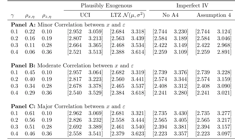
These examples document performance of plausexogandimperfectiv under one particular DGP. Below, in table 2, we consider a range of DGPs where we vary γ
(within each panel), and µ (across each panel). Here, γ refers to the failure of the exclusion restriction with which Conley et al. (2012) are concerned, and the resulting correlations betweenxandη (the compound error term) andz andη with which Nevo and Rosen (2012b) are concerned are displayed in subsequent columns. Bounds are then documented under 2 cases in Conley et al. (2012) (the UCI and LTZ approach, each with correctly specified priors), and 2 cases in Nevo and Rosen (2012b) (with and without assumption 4). In the case of Nevo and Rosen (2012b), the assumptions for “No A4” will be met providing that the sign onρx,η andρz,η are the same, and will be
met for “Assumption 4” only ifρx,η≥ρz,η.
The bounds produced in each case on the endogenous variable of interest are pre-sented in table 2. In nearly all simulations, the bounds include the true value ofβ= 3. The only cases in which this is not seen is with those in the right-most columns at the bottom of panel A. This is to be expected, given that in this case, the assumptions un-derlying the bounds (Assumption 4 of Nevo and Rosen (2012b)) are not met, and hence the imperfectiv command should correctly have been run with the noassumption4
option. In each circumstance, the Conley et al. (2012) bounds contain the true parame-ter, but this is dependent on correctly specifying the prior overγ, as we ensure in table 2. Given that in practice, knowing the true prior forγis an empirical challenge (see for example Bhalotra and Clarke (2016)), conservative assumptions onγmay be preferred.
Table 2: Performance of Various Bounds under Monte Carlo Simulation
Plausibly Exogenous Imperfect IV
γ ρx,η ρz,η UCI LTZN(µ, σ2) No A4 Assumption 4
Panel A: Minor Correlation betweenxandε
0.1 0.22 0.10 [2.952 3.059] [2.684 3.318] [2.744 3.230] [2.744 3.124] 0.2 0.16 0.19 [2.807 3.213] [2.563 3.439] [2.584 3.189] [2.584 3.046] 0.3 0.11 0.28 [2.664 3.365] [2.468 3.534] [2.422 3.149] [2.422 2.968] 0.4 0.06 0.36 [2.521 3.513] [2.388 3.614] [2.259 3.109] [2.259 2.891]
Panel B:Moderate Correlation betweenxand ε
0.1 0.45 0.10 [2.957 3.064] [2.682 3.319] [2.739 3.376] [2.739 3.228] 0.2 0.40 0.19 [2.817 3.223] [2.560 3.441] [2.574 3.344] [2.574 3.159] 0.3 0.34 0.28 [2.678 3.378] [2.465 3.537] [2.408 3.312] [2.408 3.090] 0.4 0.29 0.36 [2.540 3.529] [2.384 3.618] [2.241 3.280] [2.241 3.021]
Panel C:Major Correlation betweenxandε
0.1 0.61 0.10 [2.962 3.069] [2.681 3.321] [2.735 3.430] [2.735 3.277] 0.2 0.56 0.19 [2.826 3.232] [2.558 3.444] [2.565 3.405] [2.565 3.217] 0.3 0.51 0.28 [2.692 3.389] [2.461 3.540] [2.394 3.381] [2.394 3.157] 0.4 0.46 0.36 [2.558 3.541] [2.379 3.623] [2.223 3.357] [2.223 3.097]
95% confidence intervals associated with the parameterβare displayed in square parentheses. The true value ofβis 3 in the DGP described in (8). The value ofγin each case is displayed in the left-hand column (between 0.1 and 0.4), and the correlation betweenxandηandzandηinferred in each case is listed in subsequent columns. Hereηrefers to the compound error term which causes endogeneity and instrumental invalidity. 1000 simulated observations are used. Different panels allow the correlation between the endogenous variablexand theεterm to vary, makingx‘more’ or ‘less’ endogenous. Confidence intervals for the Plausibly Exogenous UCI case are based on a support assumption implying that the true value of
γis at the mean, and hence is [0,2γ]. In the LTZ case, the distribution forγis assumed to be normal, with mean equal to the value of gamma, and variance equal toγ/10. Confidence intervals for Imperfect IV estimates are based on assumptions that ρx,η > 0 and ρz,η > 0 in the “No A4” case, and that
ρx,η ≥ρz,η>0 in the “Assumption 4” case. The veracity of each assumption can be determined from
Damian Clarke and Benjam´ın Matta 17
relationship between instruments and unobservables. Ideally, these assumptions should be well founded in a theory related to the nature of failure of IV validity. In the case of Nevo and Rosen (2012b), a willingness to assume that an instrument is positively or negatively related to unobservables may reflect some underlying model of selection into an instrument or of behavioural response to a particular draw of the instrumental variable. Consider briefly two well known instruments in models of human fertility: the gender mix of children, and the occurrence of twin births. In the case of gender mix of births, Dahl and Moretti (2008) document a “demand for sons”, suggesting that investments following sons may depend positively on this particular realisation of the instrumental variable. In the case of twins, Bhalotra and Clarke (2016) document a cross-cutting positive selection of twin births, where many (positive) maternal health behaviours in utero increase the likelihood of giving live births to twins (even if twin conception is random). Here, assumptions relating to a positive correlation between the instrument and unobservables seems reasonable based on positive correlations between the instrument and many hard-to-measure and frequently unobserved variables.13 As
discussed above, the willingness to assume a particular range or distribution for the failure of the exclusion restriction is also an empirical challenge. While in the case of Conley et al. (2012) bounds are constructed based on stronger assumptions than just the sign of the correlation, a benefit of this approach is that it allows for the sign to be indeterminate, if for example, one is concerned that instruments may only be “close” to exogenous but not certain of the direction in which failures of validity occur. We return to these considerations below.
Abstracting now from why identifying assumptions may be met, table 2 offers a number of lessons regarding the relative performance of Conley et al. and Nevo and Rosen bounds. Firstly, the bounds on the endogenous parameter using Conley et al. (2012)’s plausexogprocedure are approximately constant across panels (given a par-ticular value for γ), as the degree of endogeneity of xdoes not impact the estimated bounds. In the case of Nevo and Rosen (2012b), all else constant, bounds are more (less) wide when the independent variable of interest is more (less) exogenous. This owes to the fact that Nevo and Rosen (2012b) use information from the original endogenous variable to form one side of their bounds (when two-sided bounds are formed). In the limit case when assumption 4 is not assumed, the bound on the OLS estimate ofβitself is used.
Secondly, it is noted that bounds from Nevo and Rosen (2012b) are always tighter when Assumption 4 is used (in the case shown in table 2, the upper bound onβ always falls). Of course, this is not free, but rather a direct result of the assumption that z
is less endogenous than x. In the case that this is true, bounds are both tighter and contain the true parameter, but when assumption 4 is not met, bounds are tighter, but
donotcontain the true parameter.
Finally, we note that in this case, adding additional structure in the Conley et al. (2012) bounding procedure via the Local to Zero approach actually results in wider bounds. This is a direct result of the parameters assumed in each case. In the UCI case, we allow for a support of [0,2×γ] for each implementation, while the LTZ case assumes thatγ∼ N(γ, γ/10), which consistently results in a probability distribution forγwhich has a considerable probability mass outside of the values allowed in the UCI approach. This should not be seen as necessarily representative of the use of the UCI and LTZ approaches. Frequently, the LTZ approach leads to tighter bounds, given the additional structure placed on the prior forγ. Indeed, in the above simulations, if we were to use a Gaussian prior in the LTZ approach with an identical variance of a uniform spanning the UCIγminandγmaxvalues, bounds in the LTZ approach would be tighter than those
in the UCI approach. This is a direct result of placing greater weight on values closer to the true value ofγwhen using the normal prior. Unlike the Nevo and Rosen (2012b) method, the Conley et al. (2012) method allows for a prior that the instrument may be positively related, negatively related, or unrelated with the unobserved error term. However, the additional flexibility of the Conley et al. (2012) method also comes with the caveat that rather than knowing the sign of the correlation between the instrument and the error term, we must assume something about the magnitude of the failure of the exclusion restriction.
While Nevo and Rosen (2012b) are based on two assumptions and no further priors are required, (as documented in the two columns of table 2), Conley et al. (2012) bounds are based on parametric priors which can take an unlimited range of values. Thus, if using Conley et al. (2012) bounds, it may be particularly useful or illustrative to visualize bounds based on a range of values for a particular parametric prior14. This
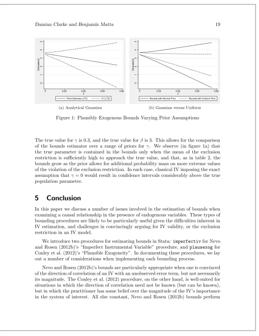
can be achieved using the graphing capabilities ofplausexog. We document an example of this code below, which produces Figure 1a below.15
. gen x = 0.33*u + 0.6*z + v . gen y3 = Beta*x + 0.3*z + u .
. quietly plausexog ltz y3 (x=z), omega(0.01) mu(0.3) graph(x) graphomega(0 0.0 > 225 0.09 0.2025 0.36 0.5625) graphmu(0 0.15 0.3 0.45 0.6 0.75) graphdelta(0 0 > .15 0.3 0.45 0.6 0.75) scheme(sj) ytitle(Estimated {&beta}) xtitle({&delta}) > xlabel(0 "0" 0.2 "0.20" 0.4 "0.40" 0.6 "0.60" 0.8 "0.80") legend(order(1 "Poi > nt Estimate (LTZ)" 2 "CI (LTZ)")) ylabel(0(1)5)
Figure 1a assumes a Gaussian (Normal) prior forγ in the LTZ approach of Conley et al. (2012), however varying the mean and variance. Bounds at each point on the graph are based on the assumption thatγ∼ N(δ, δ2). Figure 1b compares the bounds from the
Gaussian prior to bounds based on a uniform prior which assumes thatγ∼U(0,2×δ).
14. A comprehensive example of this procedure is provided in the original Conley et al. (2012, p. 267) paper. We show how to replicate a portion of their results using theplausexogado in Appendix 1.2.
Damian Clarke and Benjam´ın Matta 19
0
1
2
3
4
5
Estimated
β
0 0.20 0.40 0.60 0.80
δ
Point Estimate (LTZ) CI (LTZ)
(a) Analytical Gaussian
0
1
2
3
4
5
Estimated
β
0 0.20 0.40 0.60 0.80
δ
Bounds with Normal Prior Bounds with Uniform Prior
[image:20.612.46.574.54.740.2](b) Gaussian versus Uniform
Figure 1: Plausibly Exogenous Bounds Varying Prior Assumptions
The true value forγis 0.3, and the true value forβ is 3. This allows for the comparison of the bounds estimator over a range of priors forγ. We observe (in figure 1a) that the true parameter is contained in the bounds only when the mean of the exclusion restriction is sufficiently high to approach the true value, and that, as in table 2, the bounds grow as the prior allows for additional probability mass on more extreme values of the violation of the exclusion restriction. In each case, classical IV imposing the exact assumption thatγ= 0 would result in confidence intervals considerably above the true population parameter.
5
Conclusion
In this paper we discuss a number of issues involved in the estimation of bounds when examining a causal relationship in the presence of endogenous variables. These types of bounding procedures are likely to be particularly useful given the difficulties inherent in IV estimation, and challenges in convincingly arguing for IV validity, or the exclusion restriction in an IV model.
We introduce two procedures for estimating bounds in Stata: imperfectivfor Nevo and Rosen (2012b)’s “Imperfect Instrumental Variable” procedure, andplausexogfor Conley et al. (2012)’s “Plausible Exogeneity”. In documenting these procedures, we lay out a number of considerations when implementing each bounding process.
relatively better when the endogenous variable is less correlated with unobservables, while Conley et al. (2012) bounds perform equally well regardless of the correlation be-tween the endogenous variable of interest and unobservables. Finally, while Conley et al. (2012) bounds are often based on more parametric or otherwise stronger assumptions related to the unobservable behaviour of IVs, it is simple to undertake sensitivity test-ing of estimated bounds’ stability to changes in these assumptions, and such sensitivity tests are encouraged when dealing with questionable IVs.
Damian Clarke and Benjam´ın Matta 21
6
References
Angrist, J. D., and W. N. Evans. 1998. Children and Their Parents’ Labor Supply: Evidence from Exogenous Variation in Family Size. American Economic Review 88(3): 450–77.
Angrist, J. D., and A. B. Krueger. 1991. Does Compulsory School Attendance Affect Schooling and Earnings? The Quarterly Journal of Economics106(4): 979–1014.
Angrist, J. D., and J.-S. Pischke. 2008. Mostly Harmless Econometrics: An Empiricist’s Companion. Princeton University Press.
Bekker, P., A. Kapteyn, and T. Wansbeek. 1987. Consistent Sets of Estimates for Re-gressions with Correlated or Uncorrelated Measurement Errors in Arbitrary Subsets of all Variables. Econometrica55(5): 1223–1230.
Bhalotra, S. R., and D. Clarke. 2016. The Twin Instrument. IZA Discussion Papers 10405, Institute for the Study of Labor (IZA).
Bound, J., D. A. Jaeger, and R. M. Baker. 1995. Problems with instrumental vari-ables estimation when the correlation between the instruments and the endogenous explanatory variable is weak.Journal of the American Statistical Association90(430): 443–450.
Buckles, K. S., and D. M. Hungerman. 2013. Season of Birth and Later Outcomes: Old Questions, New Answers. The Review of Economics & Statistics95(3): 711–724.
Conley, T. G., C. B. Hansen, and P. E. Rossi. 2012. Plausibly Exogenous. The Review of Economics and Statistics 94(1): 260–272.
Dahl, G. B., and E. Moretti. 2008. The Demand for Sons. Review of Economic Studies 75(4): 1085–1120.
Hansen, L. P. 1982. Large Sample Properties of Generalized Method of Moments Esti-mators. Econometrica50(4): 1029–1054.
Hotz, V. J., C. H. Mullin, and S. G. Sanders. 1997. Bounding Causal Effects Using Data from a Contaminated Natural Experiment: Analysing the Effects of Teenage Childbearing. Review of Economic Studies64(4): 575–603.
Kang, H., A. Zhang, T. T. Cai, and D. S. Small. 2016. Instrumental Variables Estimation With Some Invalid Instruments and its Application to Mendelian Randomization. Journal of the American Statistical Association 111(513): 132–144.
Kitagawa, T. 2015. A Test for Instrument Validity. Econometrica83(5): 2043–2063.
Koles´ar, M., R. Chetty, J. Friedman, E. Glaeser, and G. W. Imbens. 2015. Identification and Inference With Many Invalid Instruments. Journal of Business and Economic Statistics 33(4): 474–484.
Leamer, E. E. 1981. Is it a Demand Curve, Or Is It A Supply Curve? Partial Identifica-tion through Inequality Constraints. The Review of Economics and Statistics63(3): 319–327.
Manski, C. F., and J. V. Pepper. 2000. Monotone Instrumental Variables: With an Application to the Returns to Schooling. Econometrica 68(4): 997–1010.
———. 2009. More on monotone instrumental variables. Econometrics Journal 12: S200–S216.
Nevo, A., and A. Rosen. 2008. Identification with imperfect instruments. CeMMAP working papers CWP16/08, Centre for Microdata Methods and Practice, Institute for Fiscal Studies.
———. 2012a. Replication data for: Identification With Imperfect Instruments. http://hdl.handle.net/1902.1/18721.
———. 2012b. Identification With Imperfect Instruments. The Review of Economics and Statistics 94(3): 659–671.
Rosenzweig, M. R., and K. I. Wolpin. 1980a. Testing the Quantity-Quality Fertility Model: The Use of Twins as a Natural Experiment. Econometrica48(1): 227–40.
———. 1980b. Life-Cycle Labor Supply and Fertility: Causal Inferences from Household Models. Journal of Political Economy 88(2): 328–348.
———. 2000. Natural “Natural Experiments” in Economics. Journal of Economic Literature 38(4): 827–874.
Rosenzweig, M. R., and J. Zhang. 2009. Do Population Control Policies Induce More Human Capital Investment? Twins, Birth Weight and China’s One-Child Policy. Review of Economic Studies 76(3): 1149–1174.
Rossi, P. 2015. bayesm: Bayesian Inference for Marketing/Micro-Econometrics. https://cran.r-project.org/web/packages/bayesm/index.html. Accessed: 2017-06-16.
Rossi, P. E., T. G. Conley, and C. B. Hansen. 2012. Replication data for: Plausibly Exogenous. http://hdl.handle.net/1902.1/18022.
Rubin, D. 1974. Estimating Causal Effects of Treatments in Randomized and Nonran-domized Studies. Journal of Educational Psychology 66(5): 688–701.
Damian Clarke and Benjam´ın Matta 23
Small, D. S. 2007. Sensitivity Analysis for Instrumental Variables Regression with Overi-dentifying Restrictions. Journal of the American Statistical Association 102(479): 1049–1058.
Wiseman, N., and T. A. Sørensen. 2017. Bounds with Imperfect Instruments: Leverag-ing the Implicit Assumption of Intransitivity in Correlations. IZA Discussion Papers 10646, Institute for the Study of Labor (IZA).
About the authors
Damian Clarke is an Associate Professor at The Department of Economics of The Universidad de Santiago de Chile, and a research associate at the Centre for the Study of African Economies, Oxford.
Benjam´ın Matta is a final year Master student in the Master in Economic Sciences at the Universidad de Santiago de Chile.
Acknowledgments
Appendices
1
Empirical Examples Using Original Data
We illustrate the performance of each of theimperfectivandplausexogprograms in Stata by replicating empirical examples from Nevo and Rosen (2012b) and Conley et al. (2012). These use data from the original papers16and the syntax of each command as laid out in section 3.
1.1
Nevo and Rosen (2012b)’s Demand for cereal Example
Below we replicate the bounds calculated by Nevo and Rosen (2012b) in their empirical application examining the demand for cereal. We use the imperfectiv command de-scribed above to calculate bounds. This syntax replicates the results in table 2 of Nevo and Rosen (2012b, p. 667), and in particular columns 3 and 4 where the Imperfect IV methodology is used.
We first show the case where “Assumption 4” is not imposed, and output bounds on both the endogenous and each exogenous variable, and then replicate the results as-suming that “Assumption 4” holds. In the second case, we only display the bounds on the endogenous variable of interest using theshortoption to simplify output. We note that in each case the results displayed here are marginally different (at the third deci-mal place) given that theimperfectiv command estimates 2SLS results using Stata’s currentivregresscommand, in place of the now outdated ivregcommand. If using
ivreg, bounds replicate those in Nevo and Rosen (2012b) exactly.
(Continued on next page)
Damian Clarke and Benjam´ın Matta 25
. use NevoRosen2012.dta
(Nevo and Rosen´s (2012) REStat cereal demand example) .
. replace addv=addv/10 (986 real changes made)
. local w addv bd1 bd2 bd3 bd4 bd5 bd6 bd7 bd8 bd9 bd10 bd11 bd12 bd13 bd14 bd1 > 5 bd16 bd17 bd18 bd19 bd20 bd21 bd22 bd23 bd24 bd25 dd2 dd3 dd4 dd5 dd6 dd7 > dd8 dd9 dd10 dd11 dd12 dd13 dd14 dd15 dd16 dd17 dd18 dd19 dd20 sfdum . gen z1=p_bs
. replace z1=p_sf if city==7 (495 real changes made) .
. imperfectiv y `w´ (price=z1 qavgp), prop5 noassumption
Nevo and Rosen (2012)´s Imperfect IV bounds Number of obs = 990 Variable Lower Bound Upper Bound
price -11.4 -2.363483 addv .146914 .418325 bd1 .033972 .599707 bd2 .455624 .298904 bd3 .382829 .450718 bd4 .187206 .401833 bd5 .605444 -.492812 bd6 -.125019 -.27417 bd7 .202934 -.19722 bd8 -.530749 -.864742 bd9 -.386157 -.807136 bd10 .894826 .716074 bd11 .4386 .373726 bd12 -.709916 -.558852 bd13 .750836 .23102 bd14 -.010961 -.316191 bd15 -.000558 -.619963 bd16 .405134 -1.042088 bd17 -.521734 -.887364 bd18 -.05868 -.505367 bd19 -.224799 -.370595 bd20 .498622 -.156238 bd21 -.763825 -.882123 bd22 .191673 -.503372 bd23 -.605655 -.555918
bd24 0 0
dd16 -.031882 -.025253 dd17 .092846 .112414 dd18 .089866 .140122 dd19 .105029 .131951 dd20 -.009224 .003433 sfdum -.097125 -.268704
. imperfectiv y `w´ (price=z1 qavgp), prop5 short
Nevo and Rosen (2012)´s Imperfect IV bounds Number of obs = 990 Variable Lower Bound Upper Bound
price -11.4 -4.082247
1.2
Conley et al. (2012)’s 401(K) Example
Below we replicate the plausibly exogenous bounds calculated by Conley et al. (2012) in their empirical application examining the effect of participation in 401(k) on asset accumulation. We use theplausexogcommand described in section 3 to calculate local to zero (ltz) bounds.
. use Conleyetal2012
(Conely et al´s (2012) REStat for 401(k) participation)
. local xvar i2 i3 i4 i5 i6 i7 age age2 fsize hs smcol col marr twoearn db pira > hown
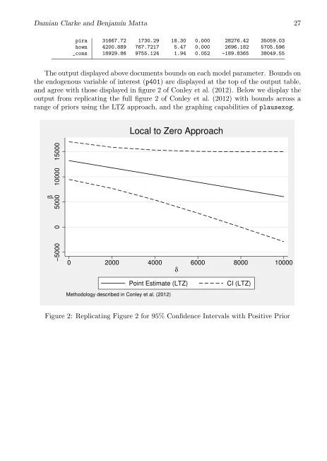
. plausexog ltz net_tfa `xvar´ (p401 = e401), omega(25000) mu(0) level(.95) vce > (robust) graph(p401) graphmu(1000 2000 3000 4000 5000) graphomega(333333.33 1 > 333333.3 3000000 5333333.3 8333333.3) graphdelta(2000 4000 6000 8000 10000) Estimating Conely et al.´s ltz method
Exogenous variables: i2 i3 i4 i5 i6 i7 age age2 fsize hs smcol col marr twoearn > db pira hown
Endogenous variables: p401 Instruments: e401
Damian Clarke and Benjam´ın Matta 27
pira 31667.72 1730.29 18.30 0.000 28276.42 35059.03 hown 4200.889 767.7217 5.47 0.000 2696.182 5705.596 _cons 18929.86 9755.124 1.94 0.052 -189.8365 38049.55
The output displayed above documents bounds on each model parameter. Bounds on the endogenous variable of interest (p401) are displayed at the top of the output table, and agree with those displayed in figure 2 of Conley et al. (2012). Below we display the output from replicating the full figure 2 of Conley et al. (2012) with bounds across a range of priors using the LTZ approach, and the graphing capabilities ofplausexog.
−5000
0
5000
10000
15000
β
0 2000 4000 6000 8000 10000
δ
Point Estimate (LTZ) CI (LTZ)
Methodology described in Conley et al. (2012)
[image:28.612.69.532.71.723.2]