Munich Personal RePEc Archive
Poverty in Malawi: Policy Analysis with
Distributional Changes
Mussa, Richard
Department of Economics, Chancellor College, University of Malawi
4 January 2017
Poverty in Malawi: Policy Analysis with
Distributional Changes
Richard Mussa
4 January 2017
Abstract
This paper addresses an issue which has hitherto been ignored in the existing studies on poverty and its correlates. Existing poverty studies ignore the fact that changes in the correlates of poverty may not only a¤ect the average level of con-sumption, but may also a¤ect the distribution of consumption. The paper develops methods for addressing this weakness. Using Malawian data from the Third In-tegrated Household Survey, the empirical application of the methods suggest that ignoring these distribution e¤ects leads to mismeasurement both quantitatively and qualitatively of policy interventions on poverty. It is found that an additional year of female education for urban households without distributional changes reduces the poverty headcount by 7.6%, and the reduction almost doubles to 11.4% with distributional e¤ects. A similar pattern is observed for the rural simulation. This in turn suggests that policy conclusions based on the existing methods might be misleading.
Keywords: Poverty; distribution; Malawi
1
Introduction
Global poverty has been declining since the 1990s; there are however disagreements about the exact magnitudes of the declines. The di¤erence in the size of the declines is primarily explained by whether one uses national accounts data or household survey data. Studies using national accounts data (e.g..Martin (2002, 2006), and Pinkovskiy and Sala-i-Martin (2009, 2014, 2016)) point to much larger declines in global poverty while studies based on household survey data indicate modest declines (e.g. Chen and Ravallion (2001, 2004, 2010)). What is also evident from these studies is that Sub-saharan Africa lags behind all other regions in terms of the pace of poverty reduction.
This aggregated picture about Sub-saharan Africa hides alot of diversity in terms poverty reduction within the region. The impact of the recent impressive economic growth in Sub-saharan Africa on poverty has been mixed. Growth has led to signi…cant poverty reduction in countries such as Ethiopia, Ghana, Uganda, and Rwanda while the same
growth has been associated with no reduction or indeed a worsening of poverty in countries including Madagscar, Kenya, and Nigeria (Arndt et al., 2016). Another phenomenon which has characterised growth in Sub-Saharan Africa is that it has been accompanied by growing inequality in some countries such as Kenya, Uganda, and Zambia (Fosu, 2015).
Despite these positive trends in poverty reduction, understanding the drivers of poverty especially in Sub-saharan Africa is still important and relevant today as it was two decades.ago. Knowledge of what factors determine poverty is important for poverty reduction. A number of studies have identi…ed factors which in‡uence poverty (Grootaert, 1997; Mukherjee and Benson, 2003; Datt and Jollife, 2005; Zhang and Wan, 2006; Cruces and Wodon, 2007; Gunther and Harttgen, 2009; Echevin, 2012; Mason and Smale, 2013). A de…ning weakness of the existing poverty studies is that in analysing the correlates of poverty they narrowly focus on how the changes in the mean of a particular correlate in‡uences poverty. These studies thus ignore the fact that changes in the correlates of poverty do not only a¤ect poverty through the direct channel of changing the average level of consumption or income, but can also a¤ect poverty indirectly by changing the distribution of consumption or income.
In light of this research gap, the paper makes two contributions to the poverty liter-ature. The …rst contribution is that this paper goes beyond this narrow focus and looks at both the direct channel (a mean e¤ect) and the indirect channel (an inequality e¤ect) of determinants of poverty. Precisely, it augments existing poverty simulation methods (see e.g. Datt and Jollife (2005) and Mukherjee and Benson (2003)) by more realistically accounting for both mean and inequality e¤ects. These proposed changes to the basic linear simulation model ensure a more accurate measurement of the impact of simulated policy interventions on poverty.
The second contribution is that the paper uses the proposed methods to re-examine determinants of poverty in Malawi. The empirical application of the methods is based on data from the Third Integrated Household Survey (IHS3). The results con…rm that ignoring these distribution e¤ects leads to mismeasurement both quantitatively and qual-itatively of policy interventions on poverty. This in turn implies that policy conclusions based on the existing methods might be misleading.
The rest of the paper is structured as follows. Section ?? looks at trends in poverty, inequality, and economic growth in Malawi. Section 3 presents the methodology and a description of the data and variables used. This is followed by the empirical results in Section 4. Finally, Section 5 concludes.
2
Growth, Inequality, and Poverty in Malawi
and 2014. The economy grew at an average annual rate of 6.2% between 2004 and 2007, and marginally decelerated to an average growth of 6.1% between 2008 and 2014. Over the same period, the agriculture sector was by far Malawi’s most important contributor to economic growth, with a contribution averaging 34.0% to overall GDP growth. Given that economic growth was primarily driven by growth in the agriculture sector, and considering that about 90% of Malawians live in farm households (Benin et al. 2012), one would expect that this impressive growth would lead to signi…cant reductions in poverty.
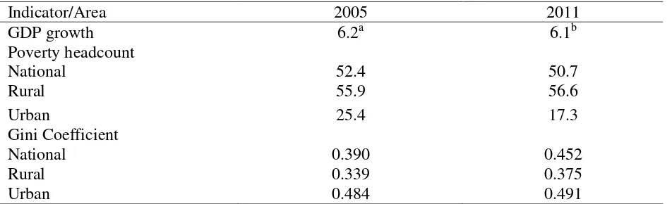
Poverty statistics however indicate that the high economic growth rates could only translate into marginal poverty reduction. The poverty …gures in Table 1 show that the percentage of poor people in Malawi was 52.4% in 2004, and slightly declined to 50.7% in 2011. Interestingly, the high economic growth rate had contrasting e¤ects on rural and urban poverty. For the period 2004-2011, the poverty headcount in rural areas minimally increased from 55.9% to 56.6% while urban poverty declined from 25.4% to 17.3%. Ironically, this dismal poverty reduction performance coincided with the Farm Input Subsidy Program (FISP), which every year provides low-cost fertilizer and improved maize seeds to poor smallholders who are mostly rural based (Chirwa and Dorward, 2013). Implementation of the FISP started in the 2005/6 cropping season, and in the 2012/13 …nancial year, the programme represented 4.6% of GDP or 11.5% of the total national budget (World Bank, 2013).
The high economic growth rates did not only fail to lead to substantial poverty re-duction but also worsened income inequality. Table 1 shows that nationally, the Gini coe¢cient increased from 0.390 in 2004 to 0.452 in 2011. The magnitude of the disequal-ising e¤ect of growth varies with location. It was more pronounced in rural areas which saw the Gini coe¢cient increase from 0.339 in 2004 to 0.375 in 2011 while the urban Gini coe¢cient rose from 0.484 to 0.491 over the same period. It can thus be concluded that many people did not bene…t from the high economic growth registered by Malawi; suggesting that growth was not inclusive. Further to this, rural households compared to their urban counterparts were the most excluded from the bene…ts of the high economic growth.
3
Methods
3.1
Distribution-Neutral Changes in the Poverty Headcount
cluster/community are likely to be dependent because they are exposed to a wide range of common community factors such as the same traditional norms regarding the roles of men and women. This dependency means that standard errors from a standard linear regression model are downward biased, and inferences about the e¤ects of the covariates may lead to many spurious signi…cant results (Hox, 2010; Cameron and Miller, 2015).
I model these common community traits as random e¤ects. Suppose that the ith
household (i= 1::::Mj) resides in the jth (j = 1::::Jl) community, then the determinants
of consumption expenditure allowing for spatial community random e¤ects can be modeled using the following two level linear regression
lnyij = 0xij+ 0qj+uj+"ij (1)
where; and are coe¢cients,xij andqj are observed household level and community
level characteristics respectively, uj N(0; 2u) are community-level spatial e¤ects
(ran-dom intercepts), assumed to be uncorrelated across communities, and uncorrelated with covariates, and "ij N(0; 2") is a household-speci…c idiosyncratic error term assumed
to be uncorrelated across households, and uncorrelated with covariates. uj and "ij are
assumed to be independent. The assumptions aboutuj and"ij imply that ij N 0; 2
where ij =uj+"ij and 2 = 2u+ 2": Thus, the overall error variance is partitioned into
two components, and this leads to an intracluster correlation coe¢cient (ICC), = 2u
2; which measures the strength of clustering within the community. If unobserved di¤erences between communities matter more than unobserved di¤erences within communities, the ICC approaches one, and the ICC will be close to zero if the reverse holds.
After estimating the regression, the next task in this paper is to simulate changes in the aggregate levels of poverty. The goal here is to assess how policy interventions which change the determinants of poverty would a¤ect the proportion of poor people. A household is de…ned as poor if it’s per capita consumption expenditure is less than a poverty line, z:Using equation (1), and noting that ij N 0; 2 ; the probability that
a household is poor can be written as
P0ij = Prob( ij <lnz ( 0xij + 0qj)) (2) = lnz (
0x
ij + 0qj)
where ( ) is a distribution function of the standard normal distribution. Estimated values of the parameters are used to predict the probability that a household is poor. Equation (2) shows how for given values of the estimated parameters, changes in levels of covariates lead to changes in the probability that a household is poor.
impact that changes in the levels of the determinants of poverty have on the aggregate incidence of poverty. Using regression coe¢cients to assess relationships between poverty and its determinants can be di¢cult if the determinants are intrinsically interrelated. Sec-ondly, and most importantly, households face signi…cant binding constraints to reducing poverty. Government policies and programs are often put in place to remove or relax these constraints. The simulation methods can be used to demonstrate the e¤ects that various policies can have on the prevalence poverty .
A simulation model which is based on the standard linear model has been used before by Datt and Jollife (2005) in Egypt and Mukherjee and Benson (2003) in Malawi. There is however one fundamental di¤erence between what they used, and what I have derived here. Unlike the previous modeling procedures, equation (2) takes into account the hierarchical nature of the data by allowing for community level random e¤ects through the division by and not ".
The population poverty headcount, a measure of the percentage of poor people in a population, can then be computed as a weighted average of P0ij; where the weight of
each household is de…ned as the product of the survey sampling weight of the household and the number of members in the household. The weighting mechanism employed here assumes that poverty is distributed equally within the household; this assumption is obviously strong. It is however di¢cult to avoid it because individual-speci…c consumption expenditure is rarely available.
Let Pb
0 be the headcount for the base scenario; this is obtained from the regressions
which use the original values of the determinants of poverty, as per equation (1). Let
Ps
0 be the headcount for an alternative scenario arising from simulated changes in the
values of the determinants of poverty, then the impact of the simulation on the incidence of poverty is simply P0 =P0s P0b:The simulated change increases poverty if P0 >0;
and reduces poverty if P0 <0:To test for statistical signi…cance of a simulated change,
I use bootstrapped standard errors for the base and the simulated headcounts, and then use pV ar( P0) = pV ar(Ps
0) +V ar(P0b)to get the standard error of the di¤erence.
In performing the simulations, the paper focuses on those selected characteristics that are amenable to change through public policy. It is worth noting that these simulations assume that there are no general equilibrium e¤ects in the sense that changes in the determinants do not a¤ect the partial regression parameters or other exogenous variables. This assumption may be valid if the simulated changes are incremental. The interpretation of the results must therefore be looked at with this caveat in mind.
3.2
Distribution-Sensitive Changes in the Poverty Headcount
the fact that changes in the correlates of poverty may not only a¤ect the average level of consumption i.e. the numerator in equation (2), but may also a¤ect the distribution of consumption i.e. the denominator in equation (2). A failure to account for distributional changes may therefore lead to misleading conclusions about the size of the impacts of policy interventions. To accommodate consumption inequality as measured by a Gini coe¢cient, equation (2) can be respeci…ed to get
P0ij =
0
@lnz (
0x
ij + 0qj)
p
2 1 (G+1) 2
1
A (3)
where G is a Gini coe¢cient. This result uses the fact that under lognormality of a welfare indicator, a Gini coe¢cient is a monotone increasing function of ; i.e. G = 2 p
2 1 (see, e.g., Kleiber and Kotz (2003) and Cowell (2009)). This reformulation
makes it more explicit that the probability that a household is poor not only depends on household and community characteristics but also depends on the extent of inequality. It further shows that increases in inequality lead to increases in poverty.
Ignoring sampling weights for expositional purposes, the Gini coe¢cient of consump-tion is expressed as (see e.g. van Doorslaer and Koolman (2004)),
G= 2
ycov(yij; Rij) (4)
where, y = N1 Pijyij; and cov(:) is a covariance, and Rij is a fractional rank of the ith
household in the consumption distribution, with households ranked from the poorest to the richest. The Gini coe¢cient in equation (4) is a Gini coe¢cient for consumption yij,
and not the log of consumption. I consequently, re-specify the poverty equation (1) so that the dependent variable is now linear to get
yij = 0xij + 0qj +u0j +"0ij (5)
Substituting equation (5) into equation (4), yields a linear regression based Gini coe¢cient as (Wagsta¤ et al., 2003)
G=X k
k
xk
y Ck+
X
k k
qk
y Ck+
...
C (6)
where, Ck is the concentration index of a regressor. The Gini coe¢cient is decomposed
into two parts. The …rst part is the observed and explained component which is equal to a weighted sum of the concentration indices of the covariates, where the weight for regressor is simply the elasticity of yij with respect to a regressor. The second part,
Cu0
j y + C" y = ... C ;
The e¤ect of a simulated change in a regressor on the Gini coe¢cient can come from two sources; a change in the mean of the regressor, and a change in the distribution of the regressor as measured by a concentration index. The corresponding total change in the Gini coe¢cient emanating from a change in a regressor is thus given by
dG=
mean ef f ect
z }| {
1
y[ kdCk]dxk+
Inequality ef f ect
z }| {
xk
y [ kdCbk] (7)
The …rst term in square brackets represents a change in the Gini following a change in the mean of a regressor. Similarly, the second term captures the inequality e¤ect. For a community level variable, qj the corresponding change in the Gini is computed
analogously.
E¤ectively two possible poverty simulation exercises can be performed. First, one can assume away distributional changes in the covariates as in Datt and Jollife (2005) and Mukherjee and Benson (2003). Second, simulated changes in policy variables can rather more realistically be considered to have both mean and inequality e¤ects. These proposed changes to the basic linear simulation model ensure a more accurate measurement of the impact of simulated policy interventions on poverty.
3.3
Data description, poverty lines, and variables used
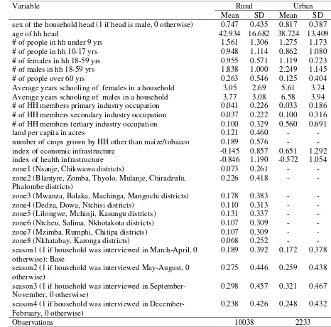
The data used in the paper are taken from the Third Integrated Household Survey (IHS3) conducted by Malawi’s National Statistical O¢ce (NSO). It is a multi-topic survey which is statistically designed to be representative at both national, district, urban and rural levels. It was conducted from March 2010 to March 2011. A strati…ed two-stage sample design was used. At the …rst stage, enumeration areas, representing communities, as de…ned in the 2008 Population Census, strati…ed by urban/rural status were selected with probability proportional size. At the second stage, systematic random sampling was used to select households.
The survey collected information from a sample of 12271 households; 2233 (represent-ing 18.2%) are urban households, and 10038 (represent(represent-ing 81.8%) are rural households. A total of 768 communities were selected from 31 districts across the country1. In each
district, a minimum of 24 communities were interviewed while in each community a total of 16 households were interviewed. In addition to collecting household level data, the survey collected employment, education, and other socio-economic data on individuals within the households. It also collected community level information on access to basic
1Malawi has a total of 28 districts. However, the IHS3 treats Lilongwe City, Blantyre City, Mzuzu
services.
In order to capture possible locational di¤erences, the paper distinguishes between rural and urban households, and I use the new annualized consumption aggregate for each household generated by Pauw et al. (2016) instead of the o¢cial aggregate as a welfare indicator i.e. the dependent variable. This choice is necessitated by the fact that the food component in the o¢cial aggregate is based on conversion factors which have been shown to have inconsistencies and errors (Verduzco-Gallo and Ecker, 2014). The computation of quantities of food consumed is based on conversion factors which are used to covert non-standard units of measurements such as pails, basins, and pieces into standard units such as kilograms and grams. The new aggregate uses a new set of conversion factors developed by Verduzco-Gallo and Ecker (2014) to generate the new food component. The o¢cial and the new consumption aggregates however have the same non-food component. I also adopt two area-speci…c poverty lines generated by Pauw et al. (2016) instead of the national level o¢cial annualised poverty line of 37002 Malawi Kwacha (MK). The poverty lines are: MK31463 for rural areas, and MK46538 for urban areas. Three groups of independent variables are included in the regressions namely; household, community, and …xed e¤ects variables. The choice of variables is guided by previous literature (e.g. Mukherjee and Benson, 2003; Datt and Jollife, 2005, Cruces and Wodon, 2007) on de-terminants of poverty. At the household level, I include a set of demographic variables: number of individuals aged below 9 years, number of individuals aged 10-17 years, number of females aged 18-59 years, number of males aged 18-59 years, the number of the elderly (above age 60) household members, the square of household size, linear and quadratic terms in the age of the household head to capture possible life cycle e¤ects, and a dummy variable for male head of household.
I include average years of schooling in a household, and this is gender-disaggregated to measure the possibility that education can have a gender-di¤erentiated e¤ect on poverty. In terms of agricultural variables, I include the number of crops the household cultivated that are not maize or tobacco, a measure of the diversity of crop cultivation. These in-clude the food crops cassava, groundnut, rice, millet, sorghum, and beans, and the cash crops cotton. Another agriculture variable included is the area of cultivated land that is owned by the household. The agriculture variables are included in the rural regressions only. The regressions also contain variables capturing the number of household members employed in the primary, secondary, and tertiary industries.
common medicines, a health clinic, a nurse, midwife or medical assistant, and groups or programs providing insecticide-treated mosquito bed nets free or at low cost. The eco-nomic infrastructure index is based on the presence of the following in a community: a perennial and passable main road, a daily market, a weekly market, a post o¢ce, a commercial bank, and a micro…nance institution.
Two sets of spatial and temporal …xed e¤ects variables are included. I include ecological zone dummies which capture zone level …xed e¤ects. There are eight agro-ecological zones. The agro-agro-ecological zone dummies control for di¤erences in land pro-ductivity, climate, and market access conditions in an area. Agro-ecological zones are rural, consequently, they only appear in the rural regression. Being an agro-based econ-omy, household welfare in Malawi may vary across the year due to possible seasonal e¤ects. I account for these variations by including three seasonal dummies re‡ecting the harvest, postharvest, and preplanting periods. I use a Wald test to check for the presence of these …xed e¤ects. Detailed de…nitions and summary statistics for all the independent variables are given in Table 2.
4
Results
4.1
Regression Results
The determinants of poverty results for rural and urban areas are reported in Table 3. Wald test results for the null of parameter homogeneity give 2 = 1828:8; suggesting that
estimating separate rural and urban regressions is appropriate. In both rural and urban areas, log likelihood tests reject the null hypothesis of no community random e¤ects. This conclusion has two implications; …rst, even after controlling for individual characteristics, there are signi…cant community-speci…c factors which a¤ect poverty, and second, estimat-ing a linear model as in for example Mukherjee and Benson (2003) and Datt and Jollife (2005) is invalid.
Gender of the household head emerges as a signi…cant correlate of poverty. Holding other things constant, female headed households are poorer than male headed households in rural areas. Precisely, their per capita consumption is 17% lower than that of male headed households. A comparison with a previous study by Mukherjee and Benson (2003) reveals some di¤erences in the relationship between gender and poverty in Malawi. Unlike the …nding in this paper, they found a rather puzzling result that in rural areas of Malawi, male headed households are poorer. A negative sign on the gender dummy in urban areas suggests that this gender di¤erence is in favour of female headed households. This rather counterintuitive …nding in urban areas is however consistent with what Mukherjee and Benson (2003) also found.
The age of the household head has a signi…cant inverted u-shaped relationship with standard of living in both areas. Precisely, I …nd that household living standards increase with the age of the head up to 65 years (90th percentile) in rural areas, and 74 years (99th percentile) in urban areas, and diminish thereafter. This means that there are signi…cant life cycle e¤ects which re‡ect increased earning capacity arising from greater experience and smoothing of consumption over one’s lifetime. This common …nding (e.g. Grootaert,1997; Datt and Jollife, 2005) is however in stark contrast to a previous study by Mukherjee and Benson (2003) who found a negative relationship between age and welfare in Malawi.
In terms of household composition, the results indicate that the coe¢cients are more negative for children aged 0-9 and the elderly (aged 60 above) than for the economically active category (i.e. 18-59 age category). This means that an increase in dependent household members leads to a larger welfare reduction than an increase in those in the economically active group. Moreover, in both areas, an increase in the household of female adults does not a¤ect per capita consumption. In contrast, the e¤ect on welfare following the addition of a male in a household is statistically signi…cant in both areas, but, it is larger in rural areas (about 31%) than in urban areas (about 22%). Considering that economic opportunities tend to favour men, one would expect a reverse pattern.
To make certain that the e¤ect of household size on consumption in Malawi is not driven by the per capita normalization, I re-estimated the poverty models by adjusting consumption for composition and economies of scale2. In both rural and urban models,
the results show that the coe¢cients on the di¤erent age-sex composition variables are negative and signi…cant, but critically, the coe¢cients are smaller in size compared to those from the per capita normalisation. For instance, in the rural model, the coe¢cient on children below 9 is -0.038 when the economies of scale parameter is 0.4, and then the coe¢cient rises to -0.239 for an economies of scale parameter of 1. Similarly, for urban areas, the coe¢cient on children below 9 is -0.029 when the economies of scale parameter is put at 0.4, it then rises to -0.226 when the parameter is 1. This means that the negative relationship between household size and welfare is not necessarily driven by the per capita normalisation but that larger households are indeed poorer than smaller ones. Besides, using the per capita measure merely leads to an overestimation of the impact of household size on poverty.
All the household education variables have statistically signi…cant positive e¤ects on per capita consumption; implying that the level of education in a household reduces the likelihood of poverty in Malawi. However, this e¤ect is gender-di¤erentiated. For instance, in rural areas and holding other factors constant, an additional year of schooling for females in a household leads to a 3.9% increase in per capita consumption while for males the corresponding e¤ect is 2.7%. Irrespective of gender, the results further indicate that there are spatial di¤erences in the size of the intrahousehold returns to education with urban areas exhibiting quantitatively larger returns than rural areas. For example, the marginal e¤ect of the years of education for females in a household is 3.9% in rural areas while it jumps to 4.6% in urban areas. This rural-urban di¤erence in the role of education perhaps re‡ects the paucity of remunerative economic opportunities in rural areas of Malawi (Mukherjee and Benson, 2003).
Employment as measured by the number of adults in a household employed in the primary, secondary, and tertiary economic sectors exhibit a mixed pattern. There are no statistically signi…cant welfare advantages to …nding employment in the primary (agricul-ture, …shing, mining, etc.) and secondary (manufacturing) sectors. However, regardless of location, employment in the tertiary sector (sales and service industries) has a statistically signi…cant, and positive e¤ect on welfare. Holding all else constant, having an additional household member employed in a tertiary industry occupation increases consumption by 21% in rural areas and by about 15% in urban areas. Notably, Mukherjee and Benson (2003) found a rather counterintuitive result that employment in a tertiary occupation does not in‡uence welfare in urban areas in Malawi.
2Instead of normalising by household size, I normalise consumption by
In terms of agriculture, the results indicate that land ownership and crop diversi-…cation have statistically signi…cant e¤ects on poverty. Holding other factors constant, an increase in cultivated area per capita by an acre increases per capita consumption in rural Malawi by 7.7%. Crop diversi…cation beyond maize and tobacco leads to a rather modest ceteris paribus increase in living standards of 2.9%. Both health and economic infrastructure in the community have a positive e¤ect on household welfare. Furthermore, in rural areas, improvements in economic infrastructure such as a perennial and passable main road, a daily market, a weekly market have a larger e¤ect on welfare than health infrastructure such as clinics and nurses. However, a reverse pattern is observed in urban areas.
There are some di¤erences in the results of this paper and a previous study by Murkherjee and Benson (2003). These di¤erences merit some comment. There are three possible explanations for these di¤erences. First, it could be driven by di¤erences in the consumption aggregates used in the two studies. Due to di¤erences in consumption in-formation collected, the consumption aggregate used by Murkherjee and Benson (2003) which was from the …rst integrated household survey is not comparable to the one used in this study which is taken from the third integrated household survey. Second, it could also be that these di¤erences re‡ect structural changes since this study is being done two decades after that of Mukherjee and Benson (2003). Finally, as the Wald test results have shown, estimating a linear model as was the case with Mukherjee and Benson (2003) is problematic, so the di¤erence could be due to fact this paper is using a superior model set up. The paper does not to attempt isolate and interrogate further which explanation drives these di¤erences by the two studies.
4.2
Simulation Results
There are ten simulations focusing on changes in population, education, employment, and agriculture. Precisely, the study simulates what would happen to the incidence of poverty under each one of the interventions. Before running these simulations a reference point or base simulation is necessary since the predicted levels of poverty are not directly comparable to the actual levels of poverty (Mukherjee and Benson, 2003; Datt and Jollife, 2005). This arises from the fact that the correlates of poverty are not perfect predictors of poverty. The base scenario is obtained from the regressions which use the original values of the determinants of poverty.
a¤ected by the simulation. Broadly, accounting for distributional e¤ects leads to more statistically signi…cant and quantitatively larger poverty changes.
The …rst two simulations are essentially population related interventions, and they involve (a) adding a child if there is no child in a household, and (b) adding a child to all households. These simulations lead to statistically signi…cant increases in the rural and urban poverty headcounts over the base scenario. Simulation 1 is a more targetted approach as it involves adding a child to households with no children, and this is associated with an increase in the rural poverty headcount of 12.3% without distribution e¤ects. The headcount jumps by 16.4% when distribution e¤ects are included. Similarly, the urban headcount increases by 13% without distribution e¤ects and then rises by 21.4% when the distributional changes are accounted for.
Simulation 2 examines the impact of adding a child to all households on the incidence of poverty, and as would be expected, this leads to an even larger increase in the poverty incidence. The urban headcount for instance increases by 65.2% without distributional e¤ects and then goes up by 80.2% after including distributional e¤ects. The correspond-ing changes in the incidence of poverty for rural areas are 54.4% and 54.8% with and without distributional e¤ects respectively. This implies that under the two simulations and regardless of whether or not one allows for distribution e¤ects, urban areas experience a larger increase in the poverty headcount than rural areas. This positive relationship be-tween children and poverty is consistent with previous studies (e.g. Eastwood and Lipton, 1999; Mussa, 2014).
Simulations 3 to 6 explore what would happen if there was an increase in average years of schooling in households. The results indicate that regardless of location, the four education simulations lead to lower levels of poverty as compared to the base scenario. Moreover, the sizes of the impacts increase as one moves from not controlling for distrib-utional e¤ects to adjusting for distribdistrib-utional e¤ects. For example, under simulation 3, an additional year of female education for urban households without distributional changes reduces the headcount by 7.6%, and the reduction almost doubles to 11.4% with distrib-utional e¤ects. A similar pattern is replicated for the rural simulation. This means that a failure to account for distributional e¤ects leads to a gross underestimation of the impact of potential education policy interventions.
the urban poverty headcount by 21.4% compared to 22.7% for females.
In addition to the gender di¤erentials in the impacts of the interventions, all the education simulations show that the reductions in the poverty headcounts are more pro-nounced in urban areas than in rural areas. Notably, there is an interaction between gender and location in terms of the size of the gender di¤erence in the impact of sim-ulated changes in schooling on poverty. For instance, after adjusting for distributional changes, the urban gender gap in the impact of a two-year increase in male education is 1.3 percentage points higher than that of female education while the rural gap of a two-year increase in female education is 3.7 percentage points higher than of male education.
It bears mentioning that there is potential for overestimating the impact of increas-ing education on poverty especially the two-year increase in years of education which is quite signi…cant in size (Datt and Jollife, 2005). Two factors could be at play and both could lead to an upward bias of the results; …rst, such an increase in education could also lead to a decline in the return to education through an increase in educated labour supply, and secondly, the returns to education may be confounded by innate abilities of household members. This …nding is nonetheless relevant for gender policy as it indicates that education interventions which deliberately seek to improve women’s education have signi…cant potential for reducing poverty in Malawi.
Simulations 7 and 8 deal with employment, and they consider the potential poverty-reduction impacts of hypothetical movements of a household member from a primary industry to a tertiary industry, and from a secondary industry to a tertiary industry. The simulation results suggest that changing the structure of employment has a signi…cant potential for reducing poverty in Malawi. There is a clear hierarchy, moving from primary to tertiary as compared to a movement from secondary to tertiary is associated with lower reductions in rural and urban poverty. Furthermore, this pattern is more evident when distributional changes are accounted for.
interven-tion leads to a decline in the rural poverty headcount of 3.9%. Simulainterven-tion 10 represents a further increase in crop diversi…cation by agriculture households from 0 or 1 to 2, and this doubling of crop diversi…cation induces a drop in the rural poverty headcount by 8.4%.
5
Concluding Remarks
This paper addresses an issue which has hitherto been ignored in the existing studies on poverty and its correlates. Existing poverty studies ignore the fact that changes in the correlates of poverty may not only a¤ect the average level of consumption, but may also a¤ect the distribution of consumption. The paper has developed methods for address-ing this weakness. Usaddress-ing Malawian data from the Third Integrated Household Survey, the empirical application of the methods suggest that ignoring these distribution e¤ects leads to mismeasurement both quantitatively and qualitatively of policy interventions on poverty.
It has been found that an additional year of female education for urban households without distributional changes reduces the headcount by 7.6%, and the reduction almost doubles to 11.4% with distributional e¤ects. A similar pattern is observed for the rural simulation. This in turn suggests that policy conclusions based on the existing methods might be misleading. Furthermore, it has been shown that an interaction exists between gender and location in terms of the size of the gender di¤erence in the impact of simulated changes in schooling on poverty. In urban areas a two-year increase in male education leads to a reduction in the headcount which is 1.3 percentage points higher than that of female education, in contrast, for rural areas a similar increase in female education is associated with a reduction in poverty which is 3.7 percentage points higher than of male education.
References
Arndt, C, McKay, A. and Tarp, F. 2016. "Synthesis: Two cheers for the African growth renaissance" in: Arndt C, McKay A, and F. Tarp (eds), Growth and Poverty in Sub-Saharan Africa, Oxford University Press: Oxford; p. 89-111.
Asselin LM. 2002. Multidimensional poverty: Composite indicator of multidimensional poverty. Levis, Quebec: Institut de Mathematique Gauss.
Blasius J, Greenacre M. 2006. Correspondence analysis and related methods in practice. In M.Greenacre, and J. Blasius (Eds.), Multiple correspondence analysis and related methods (pp. 3-40). London: Chapman and Hall.
Cameron AC and Miller DL. 2015. A Practitioner’s Guide to Cluster-Robust Inference, Journal Human Resources, 50:317-372.
Chen, S, and Ravallion, M. 2001. How Did the World’s Poorest Fare in the 1990s?,Review of Income and Wealth, 47: 283-300.
Chen, S, and Ravallion, M. 2004. How Have the World’s Poorest Fared since the Early 1980s?, World Bank Research Observer, 19: 141-169.
Chen, S, and Ravallion, M. 2010. The Developing World Is Poorer Than We Thought, but No Less Successful in the Fight against Poverty,Quarterly Journal of Economics 125: 1577-1625.
Chirwa, E. Dorward, A.2013.Agricultural Input Subsidies: The Recent Malawi Experience, Oxford: Oxford University Press.
Cruces, G., Wodon Q, 2007. Risk-adjusted poverty in Argentina: measurement and de-terminants, Journal of Development Studies,43:1189-1214.
Cowell, F. A. 2009. Measuring Inequality. New York and Oxford:: Oxford University Press.
Datt G Jolli¤e D. 2005. Poverty in Egypt: Modeling and Policy Simulations, Economic Development and Cultural Change, 53:327-346.
Eastwood, R., and M. Lipton. 1999. The impact of changes in human fertility on poverty. Journal of Development Studies 36: 1-30.
Fosu, A. K. 2015. Growth, inequality and poverty in Sub-Saharan Africa: recent progress in a global context, Oxford Development Studies 43: 44-59.
Goldstein, H. 2011. Multilevel Statistical Models: New York: John Wiley & Sons, Ltd
Grootaert, C. 1997. Determinants of Poverty in Cote d’Ivoire in the 1980s. Journal of African Economies 6: 169-96.
Hox JJ. 2010. Multilevel Analysis:Techniques and Applications, New York: Routledge.
Lanjouw, P. F. and Ravallion, M. 1995. Poverty and household size, Economic Journal, Vol. 105, pp. 1415-1434.
Lipton, M., and M. Ravallion. 1995. Poverty and policy. In Handbook of development economics, Vol. 3, ed. J. Behrman and T. N. Srinivasan. Amsterdam: North-Holland.
Mason, N. and M. Smale. 2013. Impacts of subsidized hybrid seed on indicators of eco-nomic well-being among smallholder maize growers in Zambia. Agricultural Economics 44: 1-12.
McCulloch, CE, Searle, SR and Neuhaus, JM, 2008.Generalized, Linear and Mixed Mod-els, New York: Wiley.
Mukherjee S, Benson T. 2003. The Determinants of Poverty in Malawi, 1998, World Development, 31:339-358.
Mussa, R. 2014. Impact of fertility on objective and subjective poverty in Malawi, Devel-opment Studies Research, 1: 202-222.
NSO (National Statistics O¢ce). 2005. Integrated Household Survey 2004-2005. Volume I: Household Socio-economic Characteristics, National Statistics O¢ce, Zomba, Malawi.
NSO (National Statistics O¢ce). 2012a. Integrated Household Survey 2004-2005. House-hold Socio-economic Characteristics Report, National Statistics O¢ce, Zomba, Malawi.
NSO (National Statistics O¢ce). 2012b. Quarterly Statistical Bulletin, National Statistics O¢ce, Zomba, Malawi.
Pauw K, Beck U, and Mussa R. (2016). “Did rapid smallholder-led agricultural growth fail to reduce rural poverty? Making sense of Malawi’s poverty puzzle”, in: Arndt C, McKay A, and F. Tarp (eds), Growth and Poverty in Sub-Saharan Africa, Oxford University Press: Oxford; p. 89-111.
Pinkovskiy, ML, and Sala-i-Martin, X. 2009. Parametric Estimations of the World Distri-bution of Income.NBER Working Paper No.15433.
Pinkovskiy, ML, and Sala-i-Martin, X. 2014. Africa is on Time. Journal of Economic Growth 19:311-338.
Pinkovskiy, ML, and Sala-i-Martin, X. 2016. Lights, Camera,....Income! Illuminating the National Accounts-Household Surveys Debate,The Quarterly Journal of Economics, doi: 10.1093/qje/qjw003
Sala-i-Martin, X. 2002. The Disturbing ’Rise’of Global Income Inequality, NBER Working Paper No. 8904.
Sala-i-Martin, X. 2006. The World Distribution of Income: Falling Poverty and ...Con-vergence, Period. Quarterly Journal of Economics, 121: 351-397.
van Doorslaer, E., and X. Koolman. 2004. Explaining the Di¤erences in Income-Related Health Inequalities across European Countries. Health Economics 13: 609-628.
Verduzco-Gallo, I. E. Ecker, and K. Pauw. 2014. Changes in Food and Nutrition Security in Malawi: Analysis of Recent Survey Evidence, MaSSP Working Paper 6, International Food Policy Research Institute.
Wagsta¤, A., and E. van Doorslaer. 2003. Catastrophe and Impoverishment in Paying for Health Care: with Applications to Vietnam 1993-98. Health Economics 12: 921-34.
White, H. and Masset, E. 2003. Constructing the poverty pro…le: An illustration of the importance of allowing for household size and composition in the case of Vietnam, Development and Cultural Change, Vol. 34, pp. 105-126.
Table 1: Trends and levels of economic growth, poverty, and inequality
Indicator/Area 2005 2011
GDP growth 6.2a 6.1b
Poverty headcount
National 52.4 50.7
Rural 55.9 56.6
Urban 25.4 17.3
Gini Coefficient
National 0.390 0.452
Rural 0.339 0.375
Urban 0.484 0.491
aAverage GDP growth for 2004-2007,baverage GDP growth for 2008-2014.
Table 2: Descriptive statistics of variables
Variable Rural Urban
Mean SD Mean SD
sex of the household head (1 if head is male, 0 otherwise) 0.747 0.435 0.817 0.387
age of hh head 42.934 16.682 38.724 13.409
# of people in hh under 9 yrs 1.561 1.306 1.275 1.173
# of people in hh 10-17 yrs 0.948 1.114 0.862 1.080
# of females in hh 18-59 yrs 0.955 0.571 1.119 0.723
# of males in hh 18-59 yrs 1.838 1.000 2.249 1.145
# of people over 60 yrs 0.263 0.546 0.125 0.404
Average years schooling of females in a household 3.05 2.69 5.61 3.74
Average years schooling of males in a household 3.77 3.08 6.58 3.94
# of HH members primary industry occupation 0.041 0.226 0.033 0.186
# of HH members secondary industry occupation 0.037 0.222 0.100 0.316
# of HH members tertiary industry occupation 0.100 0.329 0.560 0.691
land per capita in acres 0.121 0.460 -
-number of crops grown by HH other than maize/tobacco 0.189 0.576 -
-index of economic infrastructure -0.145 0.857 0.651 1.292
index of health infrastructure -0.846 1.190 -0.572 1.054
zone1 (Nsanje, Chikwawa districts) 0.073 0.261 -
-zone2 (Blantyre, Zomba, Thyolo, Mulanje, Chiradzulu, Phalombe districts)
0.226 0.418 -
-zone3 (Mwanza, Balaka, Machinga, Mangochi districts) 0.178 0.383 -
-zone4 (Dedza, Dowa, Ntchisi districts) 0.110 0.313 -
-zone5 (Lilongwe, Mchinji, Kasungu districts) 0.131 0.337 -
-zone6 (Ntcheu, Salima, Nkhotakota districts) 0.107 0.309 -
-zone7 (Mzimba, Rumphi, Chitipa districts) 0.107 0.309 -
-zone8 (Nkhatabay, Karonga districts) 0.068 0.252 -
-season1 (1 if household was interviewed in March-April, 0 otherwise): Base
0.189 0.392 0.172 0.378
season2 (1 if household was interviewed May-August, 0 otherwise)
0.275 0.446 0.259 0.438
season3 (1 if household was interviewed in September-November, 0 otherwise)
0.298 0.457 0.321 0.467
season4 (1 if household was interviewed in December-February, 0 otherwise)
0.238 0.426 0.248 0.432
Table 3: Determinants of poverty in Malawi, contextual e¤ects (CE) and no contextual e¤ects
Variable Rural Urban
Coefficient SE Coefficient SE
sex of the household head 0.157*** (0.014) -0.076* (0.039)
age of hh head 0.013*** (0.002) 0.027*** (0.006)
square of age of hh head -0.000*** (0.000) -0.000*** (0.000)
# of people in hh under 9 yrs -0.330*** (0.009) -0.329*** (0.020)
# of people in hh 10-17 yrs -0.329*** (0.010) -0.256*** (0.022)
# of females in hh 18-59 yrs -0.011 (0.016) -0.035 (0.029)
# of males in hh 18-59 yrs -0.311*** (0.013) -0.222*** (0.025)
# of people over 60 yrs -0.338*** (0.018) -0.143** (0.058)
square of hh size 0.017*** (0.001) 0.013*** (0.002)
Average years schooling of females in a household 0.039*** (0.002) 0.046*** (0.004)
Average years schooling of males in a household 0.027*** (0.002) 0.041*** (0.004)
# of HH members primary industry occupation 0.022 (0.026) 0.031 (0.070)
# of HH members secondary industry occupation 0.048* (0.026) 0.043 (0.042)
# of HH members tertiary industry occupation 0.210*** (0.018) 0.146*** (0.021)
land per capita in acres 0.077*** (0.014)
number of crops grown by HH other than maize/tobacco 0.029** (0.013)
index of economic infrastructure 0.085*** (0.014) 0.045* (0.027)
index of health infrastructure 0.037*** (0.010) 0.042 (0.033)
zones included Yes No
Chi2 (significance of agro-ecological zones) 262.79
-P-value of Chi2 0.00
-seasons included Yes Yes
Chi2 (significance of seasonal effects) 7.51 6.67
P-value of Chi2 0.06 0.08
Chi2 (regression) 5159.71 1231.92
P-value of Chi2 0.00 0.00
Chi2 (random effects) 847.83 314.13
P-value of Chi2 0.00 0.00
intracluster correlation coefficient (ICC) 0.16 0.24
Observations 10038 2233
Notes: Dependent variable: ln of annualised per capita household consumption in Malawi Kwacha (MK). Standard errors in parentheses. *** indicates significant at 1%; ** at 5%; and, * at 10%.
Table 4: Poverty simulations (percent change over base simulation), rural
Simulation Description
No Distribution Effect Distribution Effect
P0 % P0 %
0 Base 32.286 32.286
(0.408) (0.408)
1 Adding a child if there is no child in HH 36.249 12.3*** 37.567 16.4***
(0.418) (0.383)
2 Adding a child to all HHs 50.172 55.4*** 49.964 54.8***
(0.478) (0.339)
3 Increase average HH schooling of females by 1 year 30.334 -6.0*** 30.068 -6.9***
(0.396) (0.400)
4 Increase average HH schooling of males by 1 year 30.919 -4.2*** 30.670 -5.0***
(0.400) (0.404)
5 Increase average HH schooling of females by 2 years 28.434 -11.9*** 27.798 -13.9***
(0.383) (0.391)
6 Increase average HH schooling of males by 2 years 29.577 -8.4*** 28.998 -10.2***
(0.391) (0.399)
7 Adult moves from primary industry occupation to tertiary 23.376 -27.6*** 19.855 -38.5***
(0.342) (0.364)
8 Adult moves from secondary industry occupation to tertiary 24.529 -24.0*** 21.392 -33.7***
(0.352) (0.376)
9 Increase diversity of crops from 0 to 1 31.027 -3.9*** 31.042 -3.9***
(0.400) (0.399)
10 Increase diversity of crops to 2, if 0 or 1 29.532 -8.5*** 29.566 -8.4***
(0.390) (0.390)
Notes: Bootstrapped standard errors in parentheses. Statistical significance tests are based on absolute changes in the headcounts. *** indicates significant at 1%; ** at 5%; and, * at 10%.
Table 5: Poverty simulations (percent change over base simulation), urban
Simulation Description
No Distribution Effect Distribution Effect
P0 % Change P0 % Change
0 Base 19.789 19.789
(0.364) (0.364)
1 Adding a child if there is no child in HH 22.370 13.0*** 24.017 21.4
(0.352) (0.336)
2 Adding a child to all HHs 32.687 65.2*** 35.665 80.2
(0.463) (0.385)
3 Increase average HH schooling of females by 1 year 18.276 -7.6*** 17.535 -11.4
(0.348) (0.35–2)
4 Increase average HH schooling of males by 1 year 18.410 -7.0*** 17.670 -10.7
(0.349) (0.353)
5 Increase average HH schooling of females by 2 years 16.836 -14.9*** 15.295 -22.7
(0.331) (0.337)
6 Increase average HH schooling of males by 2 years 17.091 -13.6*** 15.556 -21.4
(0.334) (0.340)
7 Adult moves from primary industry occupation to tertiary 16.099 -18.6*** 13.203 -33.3
(0.323) (0.330)
8 Adult moves from secondary industry occupation to tertiary 16.484 -16.7*** 14.501 -26.7
(0.327) (0.334)
Notes: Bootstrapped standard errors in parentheses. Statistical significance tests are based on absolute changes in the headcounts. *** indicates significant at 1%; ** at 5%; and, * at 10%.