Munich Personal RePEc Archive
Effect of Aging on Urban Land Prices in
China
Sun, Tianyu and Chand, Satish and Sharpe, Keiran
UNSW Canberra
26 June 2018
Online at
https://mpra.ub.uni-muenchen.de/89237/
Effect of Aging on Urban Land Prices in
China
(Paper to be presented at the International Conference on Economic Modelling -
EcoMod2018 in Venice, Italy, 4th to 6th, July, 2018)
PRELIMINARY DRAFT
Tianyu Sun∗, Satish Chand and Keiran Sharpe
ABSTRACT
This paper investigates the effect of demographic changes on land prices in urban China
using an Overlapping Generation (OLG) model. The model suggests that the rapid rise in
land prices could be explained by the rise in per capita income and demographic changes.
This finding is validated by fitting the historical data of China. We then simulate land price
dynamics for China from 2000 to 2100. The simulation indicates that the rate of rise in land
prices is softening. From 2035 to 2055, the effect of demographic changes on urban land
prices in China will be close to zero. After 2055, the effect will turn to negative until the end
of this century; however, a meltdown is unlikely.
JEL classification: E21, E31, J11, R21, R31
Keywords: Aging Population; OLG Model; Urban Land Prices; Forecast
∗ Corresponding author, Tianyu.Sun@student.adfa.edu.au
Introduction
Aging population has been happening across the world. Booming research is focusing on it
because it may have a profound impact on the economy. As China is facing a significant
aging population, it is one of the best examples in examining its effect. According to the Life
Cycle Hypothesis (LCH), this demographic change indicates that more assets would be sold
by the elderly, and thus put downward pressure on the prices of houses. If true, will aging
stop the undergoing rapid rising of land price in China, or even flip it to decline? Due to the
importance of land price to both the households and macroeconomics1, the scope of this
effect should be investigated quantitatively beforehand. The results will also provide clues to
other countries that will themselves encounter the same problems.
There is a vast literature emerges discussing the linkage between demography and economic
activities2. Among the literature, the OLG model in chapter 4 is one of the first that
systematically discussed the effect of demographic changes on land prices. Most conclusions
of that chapter have not been covered in the previous research. In this chapter, we will extend
this model and simulate the land price dynamics according to the predicted demographic
changes of the United Nations (UN). This study is meaningful in at least two aspects as
follows. First, it tests the model performance in relatively realistic situations. Second, a bulk
of the literature that forecasts the land or house prices has adopted methods that are
data-driven3. This study will provide an alternative solution, which is based on economic theories,
in forecasting the dynamics of land prices.
In particular, this study attempts to quantitatively forecast the land price dynamics according
to the demographic changes from 2000 to 2100 in China. The model, as mentioned above, is
extended from the model of Chapter 4, and it includes four new ingredients as follows. First,
this model incorporates 16 age groups, covering the adulthood from 20 to 99. Each age group
has a range of five years so as to be consistent with the dataset of the UN. The multiple age
groups will allow us to simulate the demographic changes in more detail. Second, the
rural-urban migration has been taken into consideration in this model. In real situations, the land
1 For households, the land price will affect their total wealth as housing assets constitute a large part of it (Xie
and Jin 2015). In addition, the land price has a close relationship with the macroeconomic fluctuations (Liu, Wang, and Zha 2013).
2 See, for example, Cervellati and Sunde (2011), Balestra and Dottori (2011), Curtis, Lugauer, and Mark (2015),
and Muto, Oda, and Sudo (2016).
3 See, for example, Rapach and Strauss (2009) ,Gupta and Majumdar (2015), Plakandaras et al. (2015), and Wei
price dynamics we care about mainly refers to those in the urban areas, and the rapid
urbanization in China has been recognized as an important factor influencing the land price4.
Thus, this migration should be essential in our simulation. Third, instead of designing a
complicated inheritance system as exists in reality, we introduce a simple way to avoid this
discussion. The key of this method is the introduction of a government sector, and the details
are left in the corresponding section of this chapter. Lastly, the tax rate that serves as a
pay-as-you-go pension system will be flexible in this chapter, to better corresponds with the
reality.
Assuming perfect foresight of households, our baseline projection computes the transitional
path of the land prices affected by the demographic changes. To show that our model could
provide clues on the dynamics of urban land price in China, we use the projection results to
fit the historical data from 2005 to 20155. The fitted result indicates that the trend of the
historical land price can be explained from the perspective of income and demography, and
the well-fitting confirms the meaningfulness of our projection. In the out-of-sample periods,
this projection shows that the effect of demographic changes on land prices could be divided
into three periods. The first period lasts from 2000 to 2035, in which the effect stays positive.
After that, this effect would be close to zero until 2055, forming a stable period. The third
period consists the rest of this century, and the negative effect dominates in this period.
Although a long-lasting declining period is predicted, this decline can hardly be described as
a meltdown because the fall is moderate.
In addition to the baseline projection, we decompose the overall demographic changes into
the changes in three distinct sources, i.e. 1) worker population, 2) longevity and 3) age
structures. To analyse their effects, we conduct counterfactual simulations to reveal their
roles in forming the land price dynamics. In particular, the worker population is discovered to
be the main force raising the land price in China from 2000 to 2100. On the contrary, the age
structure changes will depress the land prices. The effect of longevity increase is not
significant in this simulation because its effect is absorbed by 1) the price rise beforehand,
and 2) the effect of age structure changes. The details will be provided in the corresponding
sections.
Besides, we further studied the effect of age structure changes by looking into the behaviours
of households in different age groups. To the results, we find that the per capita land demand
of households by age is conditional and varies in different circumstances. Thus, the forecasts
in the literature that are based on the historical survey data of households’ land demand could
be biased. In particular, a higher / lower growth rate of worker population will raise / depress
the per capita land demand. When longevity is higher / lower, the land demand will also be
higher / lower. For the age structure, a more / less centred age structure will imply a lower /
higher per capita land demand.
The remainder of this chapter is organized as follows. Section 2 describes the OLG model,
Section 3 presents the data, the calibration of parameters, and assumptions. The quantitative
results are shown in Section 4, including the fitting of historical data, baseline projection and
the counterfactual simulations. A discussion on the relationship between age structure and
Model
A. Demography
Our model consists of 16 age groups, covering the households’ age from 20 to 99, and each
age group spans 5 years. The households younger than 20 years are assumed not to be
participating in the land market, thus the children and young teenagers aged from 0 to 19 are
omitted from the model. Meanwhile, households older than 99 are assumed to leave the
economy system. Within the modelled age groups, those aged from 20 to 64 are assumed to
be workers as in Curtis, Lugauer, and Mark (2015), and the corresponding age groups are
numbered from 1 to 9. While the rest of the households are retirees, whose age groups are
from 10 to 16 (i.e. aged between 65 and 99). Although in practice the retirement ages differ
across genders and careers, we take a fixed retirement age for simplicity.
The cohort size dynamics of urban residents follow the following rules:
𝑁𝑁𝑡𝑡,𝑖𝑖 =𝜋𝜋𝑡𝑡,𝑖𝑖𝑁𝑁𝑡𝑡−1,𝑖𝑖−1+𝑀𝑀𝑡𝑡,𝑖𝑖 (7-1)
where 𝑁𝑁𝑡𝑡,𝑖𝑖 represents the worker population of age group 𝑖𝑖 at period 𝑡𝑡, and 𝜋𝜋𝑡𝑡,𝑖𝑖 denotes the survival rate of 𝑖𝑖 −1 age group from period 𝑡𝑡 −1 to 𝑡𝑡. The variable 𝑀𝑀𝑡𝑡,𝑖𝑖 represents the migrants of age group 𝑖𝑖 from rural to urban areas in period𝑡𝑡.
In this model, although we focus on the urban land prices, the urban population is not a
closed system because of rural-urban migration. Here, the urban residents consist of two
parts. The term 𝜋𝜋𝑡𝑡,𝑖𝑖𝑁𝑁𝑡𝑡−1,𝑖𝑖−1 denotes the urban residents that survived to period 𝑡𝑡, and the term
𝑀𝑀𝑡𝑡,𝑖𝑖 represents the immigrants.
B. Households
Preference
All households have the same preferences. They prefer consumption and land; meanwhile,
they have a dis-preference for labour supply. The land is incorporated in preferences because
it is tightly related with houses (Liu, Wang, and Zha 2013). This preference could be
described by the utility function as follows:
𝑈𝑈𝑡𝑡,𝑖𝑖 = ln�𝑐𝑐𝑡𝑡,𝑖𝑖�+𝑗𝑗𝑙𝑙 ln (𝑙𝑙𝑡𝑡,𝑖𝑖)− 𝜏𝜏𝑛𝑛𝑡𝑡,𝑖𝑖
1+𝜂𝜂 (7-2)
respectively. The consumption and land are in natural-logs, so that the utility would be
concave with respect to these factors. Meanwhile, the dis-utility of labour supply is in an
exponential form as in Iacoviello and Neri (2010) and Liu, Wang, and Zha (2013). The
parameter 𝑗𝑗𝑙𝑙 represents the preference of land. The dis-preference of labour supply are
characterized by the parameters 𝜏𝜏 and 𝜂𝜂. Because the retirees 10≤ 𝑖𝑖 ≤16 have no labour
supply, the above function could be simplified as 𝑈𝑈𝑡𝑡,𝑖𝑖 = ln�𝑐𝑐𝑡𝑡,𝑖𝑖�+𝑗𝑗𝑙𝑙 ln (𝑙𝑙𝑡𝑡,𝑖𝑖) for these age groups.
When households are at 20 years old (the beginning of the 1st age group), they will plan their
consumption, land and labour supply to maximize their utility of whole lifetime. More
concretely, the utility function of their whole lifetime is as follows:
𝑈𝑈𝑡𝑡 =� 𝛽𝛽𝑖𝑖−1
16
𝑖𝑖=1 𝜋𝜋𝑡𝑡,𝑖𝑖𝑈𝑈𝑡𝑡,𝑖𝑖
(7-3)
Here, 𝑈𝑈𝑡𝑡,𝑖𝑖 is the utility function of the ith age group as shown in Eq. (7-1) and (7-2), and the lifetime utility is the weighted sum of 𝑈𝑈𝑡𝑡,𝑖𝑖 (1≤ 𝑖𝑖 ≤ 16). The weight is characterized by the time preference of households, 𝛽𝛽, and the survival rate of households, 𝜋𝜋𝑡𝑡,𝑖𝑖. In particular, 𝜋𝜋𝑡𝑡,1 is assumed to be 1, while 𝜋𝜋𝑡𝑡,𝑖𝑖 (𝑖𝑖 ≠1) are calculated from the statistical data of the UN
(details provided in the section of data).
Budget
For the urban residents, the budget constraint when they are workers (ith age group, 1≤ 𝑖𝑖 ≤
9) is as follows:
𝑐𝑐𝑡𝑡,𝑖𝑖+𝑝𝑝𝑙𝑙,𝑡𝑡𝑙𝑙𝑡𝑡,𝑖𝑖 = (1− 𝑇𝑇)�𝑤𝑤𝑡𝑡𝑛𝑛𝑡𝑡,𝑖𝑖+𝑑𝑑𝑡𝑡�+𝑝𝑝𝑙𝑙,𝑡𝑡𝑙𝑙𝑡𝑡−1,𝑖𝑖−1 (7-4)
The left side of this equation is the per capita expenditure of this age group. The expenditure
consists of the consumption, 𝑐𝑐𝑡𝑡,𝑖𝑖, and the market value of land, 𝑝𝑝𝑙𝑙,𝑡𝑡𝑙𝑙𝑡𝑡,𝑖𝑖, where the variable 𝑝𝑝𝑙𝑙,𝑡𝑡 denotes the price of land in period 𝑡𝑡.
The right side of Eq. (7-4) represents the income of urban workers that comes from three
sources. The first source is the wage from labour supply. The wage and per capita labour
supply are denoted by 𝑤𝑤𝑡𝑡 and 𝑛𝑛𝑡𝑡,𝑖𝑖 respectively. Thus, the per capita wage earning of this age group is 𝑤𝑤𝑡𝑡𝑛𝑛𝑡𝑡,𝑖𝑖. The second source is the profit of firms. This profit is assumed to be
distributed evenly across the worker population, and the per worker profit is denoted by 𝑑𝑑𝑡𝑡.
and this transfer could be viewed as a pay-as-you-go pension system. This tax rate is assumed
to be flexible according to demographic conditions, and the details can be found in the
parameterization section below.
The last source of income comes from the market value of the land that was owned by the
households in the last period. Here, we assume that the inheritance of land is not included in
this model6. Thus, the per capita land that could be sold in period t would be 𝑙𝑙𝑡𝑡−1,𝑖𝑖−1, which is the same as the per capita land owned by this generation in the previous period. The land is
sold at the current price 𝑝𝑝𝑙𝑙,𝑡𝑡, thus the market value is 𝑝𝑝𝑙𝑙,𝑡𝑡𝑙𝑙𝑡𝑡−1,𝑖𝑖−1. In addition, the age group one that has no land owned in the previous period (𝑙𝑙𝑡𝑡−1,0 = 0), so the market value would be zero.
For the migrants of this age group, their per capita budget constraint is shown as follows:
𝑐𝑐𝑡𝑡𝑚𝑚,𝑖𝑖+𝑝𝑝𝑙𝑙,𝑡𝑡𝑙𝑙𝑡𝑡𝑚𝑚,𝑖𝑖 = (1− 𝑇𝑇)�𝑤𝑤𝑡𝑡𝑛𝑛𝑡𝑡𝑚𝑚,𝑖𝑖+𝑑𝑑𝑡𝑡𝑚𝑚�+𝑠𝑠𝑡𝑡,𝑖𝑖 (7-5)
Same as the urban residents, the migrants spend their income on consumption, 𝑐𝑐𝑡𝑡𝑚𝑚,𝑖𝑖, and land, 𝑙𝑙𝑚𝑚𝑡𝑡,𝑖𝑖. They also receive income as wage, 𝑤𝑤𝑡𝑡𝑛𝑛𝑚𝑚𝑡𝑡,𝑖𝑖, and profit distribution, 𝑑𝑑𝑡𝑡𝑚𝑚. The difference
between migrants and urban residents lies on that the migrants not owning urban land in the
previous period. However, we assume that they will bring an amount of wealth 𝑠𝑠𝑡𝑡,𝑖𝑖 when they enter the urban areas. One could rationalise it as their savings. Furthermore, we assume that
the wealth they bring with them follow the equation:
𝑠𝑠𝑡𝑡,𝑖𝑖 =𝑝𝑝𝑙𝑙,𝑡𝑡𝑙𝑙𝑡𝑡−1,𝑖𝑖−1 (7-6)
The right side of Eq. (7-6) is exactly the market value of land of urban residents. This
assumption indicates that there is no wealth inequality between urban residents and migrants.
This is a simplifying assumption that eases calculation since it means that all workers face the
same budget constraint Eq. (7.4).
Because the profit is evenly distributed to all the workers, the profit earnings of urban
residents and migrants are also equal, i.e. 𝑑𝑑𝑡𝑡𝑚𝑚 =𝑑𝑑𝑡𝑡. In addition, because the preferences of
migrants are the same as that of residents in every age group, the migrants will choose the
6 In this chapter, we assume that the land without an owner will be collected by the government, and this
same consumption, land and labour supply as the residents due to their equality7, i.e. 𝑐𝑐𝑡𝑡𝑚𝑚,𝑖𝑖 =
𝑐𝑐𝑡𝑡,𝑖𝑖,𝑙𝑙𝑡𝑡𝑚𝑚,𝑖𝑖 =𝑙𝑙𝑡𝑡,𝑖𝑖,𝑛𝑛𝑡𝑡𝑚𝑚,𝑖𝑖 = 𝑛𝑛𝑡𝑡,𝑖𝑖. Therefore, the budget constraint of workers, regardless of whether
they are residents or migrants, could be represented by the same form as Eq. (7-4).
For urban residents, the per capita budget constraint of retirees of age group 𝑖𝑖 (10≤ 𝑖𝑖 ≤ 16)
is shown as follows:
𝑐𝑐𝑡𝑡,𝑖𝑖+𝑝𝑝𝑙𝑙,𝑡𝑡𝑙𝑙𝑡𝑡,𝑖𝑖 =
1
𝑟𝑟 𝑇𝑇 (𝑤𝑤𝑡𝑡𝑛𝑛𝑡𝑡+𝑑𝑑𝑡𝑡) +𝑝𝑝𝑙𝑙,𝑡𝑡𝑙𝑙𝑡𝑡−1,𝑖𝑖−1 (7-7)
The left side of Eq. (7-7) is the expenditures of retirees. Similarly to workers, they purchase
consumption and land. The income of retirees (right side of Eq. (7-7)) could be divided into
two parts. The far RHS term is the land that they owned in the previous period, and the
market value of this land is 𝑝𝑝𝑙𝑙,𝑡𝑡𝑙𝑙𝑡𝑡−1,𝑖𝑖−1. This part is the same as that of the workers.
The remaining part is the pension income, and this part is represented by 1
𝑟𝑟 𝑇𝑇 (𝑤𝑤𝑡𝑡𝑛𝑛𝑡𝑡+𝑑𝑑𝑡𝑡) in
Eq. (7-7), where the variable 𝑛𝑛𝑡𝑡 represents the averaged labour supply per worker. In Eq.
(7-7), the parameter r denotes retiree dependent ratio8. Assuming that the pension income for
each retiree is the same, this formula can be derived by the following steps. First, all the
pension tax received from workers can be denoted by 𝑇𝑇 (𝑤𝑤𝑡𝑡𝑛𝑛𝑡𝑡𝑁𝑁𝑡𝑡+𝑑𝑑𝑡𝑡𝑁𝑁𝑡𝑡), where 𝑁𝑁𝑡𝑡 is the
total worker population. Thus, for each retiree, the pension income is 𝑇𝑇 (𝑤𝑤𝑡𝑡𝑛𝑛𝑡𝑡+𝑑𝑑𝑡𝑡)𝑁𝑁𝑡𝑡/𝑂𝑂𝑡𝑡,
where the variable 𝑂𝑂𝑡𝑡 denotes the population of retirees. Let’s define 𝑟𝑟=𝑁𝑁𝑂𝑂𝑡𝑡
𝑡𝑡, then the per
capita pension income is 1
𝑟𝑟 𝑇𝑇 (𝑤𝑤𝑡𝑡𝑛𝑛𝑡𝑡+𝑑𝑑𝑡𝑡).
The per capita budget constraint of migrant retirees (10≤ 𝑖𝑖 ≤ 16) is as follows:
𝑐𝑐𝑡𝑡𝑚𝑚,𝑖𝑖+𝑝𝑝𝑙𝑙,𝑡𝑡𝑙𝑙𝑡𝑡𝑚𝑚,𝑖𝑖 =
1
𝑟𝑟 𝑇𝑇 (𝑤𝑤𝑡𝑡𝑛𝑛𝑡𝑡+𝑑𝑑𝑡𝑡) +𝑠𝑠𝑡𝑡,𝑖𝑖 (7-8)
Here, we assume that the migrant retirees will receive the same pension income as urban
residents, and they will bring an amount of wealth 𝑠𝑠𝑡𝑡,𝑖𝑖. Similarly to workers, we assume that 𝑠𝑠𝑡𝑡,𝑖𝑖 = 𝑝𝑝𝑙𝑙,𝑡𝑡𝑙𝑙𝑡𝑡−1,𝑖𝑖−1, so there will be no wealth inequality between resident and migrant retirees.
In addition, because the households are assumed to have the same preference, residents and
7 Every household maximize the utility function according to the budget constraints. For the migrants, no matter
what value of utility function is before migration, the decisions on expenditure and labour supply depend only on the budget constraint thereafter. Because the migrants have the same wealth and preference as residents, the decisions of migrants will be the same as residents.
8 The retiree dependent ratio = the population of retirees / the population of workers. This ratio denotes the
migrants will have the same expenditure choices on consumption and land, i.e. 𝑐𝑐𝑡𝑡𝑚𝑚,𝑖𝑖 =
𝑐𝑐𝑡𝑡,𝑖𝑖,𝑙𝑙𝑚𝑚𝑡𝑡,𝑖𝑖 =𝑙𝑙𝑡𝑡,𝑖𝑖. Thus, for each retiree of age group𝑖𝑖, the per capita budget constraint can be
denoted by the Eq. (7-7).
C. Firms
In the modelling of households, the equations are denoted by per capita variables, such as per
capita consumption, land and labour supplies. However, for the simplicity of illustration, we
will use aggregate variables instead of the per capita variables in the following model
sections. These aggregate variables will be denoted using uppercase letters. For example, the
variables 𝐷𝐷𝑡𝑡 will represent the aggregate profits of firms at period 𝑡𝑡, and it equals the product
of per worker profit and worker population, i.e. 𝐷𝐷𝑡𝑡= 𝑑𝑑𝑡𝑡𝑁𝑁𝑡𝑡. Meanwhile, the aggregate labour
supply will be denoted as 𝑁𝑁𝑐𝑐,𝑡𝑡 that:
𝑁𝑁𝑐𝑐,𝑡𝑡=� 𝑛𝑛𝑡𝑡,𝑖𝑖
9
𝑖𝑖=1 𝑁𝑁𝑡𝑡,𝑖𝑖 =𝑛𝑛𝑡𝑡𝑁𝑁𝑡𝑡
(7-9)
Besides, the aggregate consumption and land of age group 𝑖𝑖 at period 𝑡𝑡 are denoted by 𝐶𝐶𝑡𝑡,𝑖𝑖 and 𝐿𝐿𝑡𝑡,𝑖𝑖. They satisfy the equations 𝐶𝐶𝑡𝑡,𝑖𝑖 = 𝑐𝑐𝑡𝑡,𝑖𝑖𝑁𝑁𝑡𝑡,𝑖𝑖 and 𝐿𝐿𝑡𝑡,𝑖𝑖 = 𝑙𝑙𝑡𝑡,𝑖𝑖𝑁𝑁𝑡𝑡,𝑖𝑖.
Technology
The production technology is assumed to have the following specification:
𝑌𝑌𝑡𝑡 =𝐴𝐴𝑡𝑡𝐾𝐾𝑡𝑡−1𝜇𝜇𝑐𝑐 𝐿𝐿𝜇𝜇𝑒𝑒𝑙𝑙,𝑡𝑡−1𝑁𝑁𝑐𝑐1−𝜇𝜇,𝑡𝑡 𝑐𝑐−𝜇𝜇𝑙𝑙 (7-10)
In each period, the production 𝑌𝑌𝑡𝑡 requires input of capital, land and labour, which are denoted
by 𝐾𝐾𝑡𝑡−1,𝐿𝐿𝑒𝑒,𝑡𝑡−1 and 𝑁𝑁𝑐𝑐,𝑡𝑡. Following Liu, Wang, and Zha (2013), the values for capital and land are those for the previous period. The production function has Cobb-Douglas form. The
parameters 𝜇𝜇𝑐𝑐 and 𝜇𝜇𝑙𝑙 denote the contribution share of capital and land respectively, and the
parameter 1− 𝜇𝜇𝑐𝑐− 𝜇𝜇𝑙𝑙 represents the share of labour income. Besides, the Total Factor
Productivity (TFP) affects the final output and is denoted by 𝐴𝐴𝑡𝑡.
Aim and budget
In the same manner as the model of Chapter 4, the firms maximize profits as follows:
𝑀𝑀𝑀𝑀𝑀𝑀 � 𝛽𝛽𝑒𝑒𝑡𝑡 ln (𝐷𝐷𝑡𝑡) 𝑡𝑡
The total profits of firms in period 𝑡𝑡 is denoted by 𝐷𝐷𝑡𝑡, and it equals the product of per worker
profit and worker population, i.e. 𝐷𝐷𝑡𝑡 = 𝑑𝑑𝑡𝑡𝑁𝑁𝑡𝑡. The time preference of firms is denoted by 𝛽𝛽𝑒𝑒.
The firms will maximize the profits according to the budget constraint as follows:
𝐷𝐷𝑡𝑡+𝐴𝐴𝐾𝐾𝑡𝑡 𝑘𝑘,𝑡𝑡
+𝑤𝑤𝑡𝑡𝑁𝑁𝑐𝑐,𝑡𝑡+𝑝𝑝𝑙𝑙,𝑡𝑡𝐿𝐿𝑒𝑒,𝑡𝑡+Φ𝑡𝑡 =𝑌𝑌𝑡𝑡+1− 𝛿𝛿k
𝐴𝐴𝑘𝑘,𝑡𝑡 𝐾𝐾𝑡𝑡−1
+𝑝𝑝𝑙𝑙,𝑡𝑡𝐿𝐿𝑒𝑒,𝑡𝑡−1 (7-12)
This budget constraint is the same as that of Chapter 4 except that we omit the housing
production sector.
In Eq. (7-12), the left-hand side of the equation is the expenditures of the firms. Besides
distributing profits 𝐷𝐷𝑡𝑡, the firms have to decide on the value of capital, 𝐾𝐾𝑡𝑡. The latter is
affected by an investment specific technology 𝐴𝐴𝑘𝑘,𝑡𝑡 as in Chapter 4. Thus, this expenditure is denoted by 𝐾𝐾𝑡𝑡
𝐴𝐴𝑘𝑘,𝑡𝑡
in Eq. (7-12). During the investment, the adjustment cost is denoted by Φ𝑡𝑡,
and its specification is the same as that of Chapter 4; that is:
Φ𝑡𝑡 =Φ(𝐾𝐾𝑡𝑡,𝐾𝐾𝑡𝑡−1) =𝜙𝜙2𝑘𝑘(𝐾𝐾𝐾𝐾𝑡𝑡
𝑡𝑡−1− 𝑔𝑔𝑘𝑘,𝑡𝑡) 2𝐾𝐾
𝑡𝑡−1 (7-13)
where the parameter 𝜙𝜙𝑘𝑘 denotes the frictions in adjusting the capital. The variable 𝑔𝑔𝑘𝑘,𝑡𝑡 represents the balance growth rate of capital at period t, and this setting makes the capital
adjustment cost equal zero along the balanced growth path.
The firms also pay workers for their labour supply. The variable 𝑁𝑁𝑐𝑐,𝑡𝑡 represents the total labour supply, and formula 𝑤𝑤𝑡𝑡𝑁𝑁𝑐𝑐,𝑡𝑡 denotes the total wage payment of the firms. In addition, the firms have to decide on the land, 𝐿𝐿𝑒𝑒,𝑡𝑡, and this expenditure is represented by the
formula𝑝𝑝𝑙𝑙,𝑡𝑡𝐿𝐿𝑒𝑒,𝑡𝑡.
The right side of Eq. (7-12) is the income of the firms. The income is from: 1) the production,
𝑌𝑌𝑡𝑡, 2) the capital owned in the last period, 𝐾𝐾𝑡𝑡−1, and 3) the land, 𝐿𝐿𝑒𝑒,𝑡𝑡−1. The capital is affected
by the depreciation rate, 𝛿𝛿k, and the investment specific technology 𝐴𝐴𝑘𝑘,𝑡𝑡, thus its value is
1−𝛿𝛿k
𝐴𝐴𝑘𝑘,𝑡𝑡 𝐾𝐾𝑡𝑡−1. The land is not affected by these factors, and its market value is 𝑝𝑝𝑙𝑙,𝑡𝑡𝐿𝐿𝑒𝑒,𝑡𝑡−1.
D. Government
In this model, instead of designing an inheritance rule of land owned by households, we
assume that the government will acquire all the land whose owners have passed away. For
owned will be transferred to government. After that, the land collected by the government
will be sold to the households and firms at the market price, 𝑝𝑝𝑙𝑙,𝑡𝑡. We assume that the government holds no land at the end of every period. Thus, the role of the government is to
re-distribute the land though the market. Lastly, all the revenue received by the government
will be spent as government expenditure (denoted by G𝑡𝑡) on the goods market.
Introducing the government into this model alleviates the need for the design of an
inheritance system. Different from the case in Chapter 4, the inheritance in multiple
generation model could affect the wealth of generations significantly. For example, suppose
that we use the same setting as in Chapter 4 that the land is inherited by the same generation
as the ones that pass away. Then, if the survival rate 𝜋𝜋𝑖𝑖,𝑡𝑡 is 0.2, then this generation will receive land that is 5 times the per capita land that they owned before. Thus, the wealth of
this generation will increase significantly and affect the households’ behaviour accordingly.
To avoid the significant behaviour changes illustrated above, we can either design a
complicated inheritance system to fit the reality or design no inheritance at all. Because the
inheritance is not the focus of our research, we choose the second option and the government
sector is introduced to collect and sell the land.
E. Equilibrium
The three markets in our model are the goods market, land market and labour market. For the
goods market, the equilibrium condition is as follows:
𝐶𝐶𝑡𝑡+ IK𝑡𝑡+ G𝑡𝑡+Φ𝑡𝑡 =𝑌𝑌𝑡𝑡+ S𝑡𝑡 (7-14)
The supply side of the goods market is represented by the right side of Eq. 7-14. The two
sources are production 𝑌𝑌𝑡𝑡 and the wealth brought by migrants S𝑡𝑡. The left side of Eq. 7-14
represents the demand of the goods market. The demand consists of consumption 𝐶𝐶𝑡𝑡,
investment IK𝑡𝑡, government expenditure G𝑡𝑡 and the adjustment cost Φ𝑡𝑡.
Here, 𝐶𝐶𝑡𝑡 denotes the aggregate consumption of all the age groups, i.e. 𝐶𝐶𝑡𝑡 =∑16𝑖𝑖=1𝐶𝐶𝑡𝑡,𝑖𝑖; IK𝑡𝑡
represents the aggregate investment that has the specification: IK𝑡𝑡= 1
𝐴𝐴𝑘𝑘,𝑡𝑡𝐾𝐾𝑡𝑡− 1−𝛿𝛿kc
𝐴𝐴𝑘𝑘,𝑡𝑡 𝐾𝐾𝑡𝑡−1; the
aggregate wealth brought by migrants is denoted by 𝑆𝑆𝑡𝑡, and it follows the specification that 𝑆𝑆𝑡𝑡 =∑16𝑖𝑖=1𝑆𝑆𝑡𝑡,𝑖𝑖.
𝐿𝐿𝑡𝑡=𝐿𝐿ℎ,𝑡𝑡+𝐿𝐿𝑒𝑒,𝑡𝑡 (7-15)
This condition is the same as that of Chapter 4, meaning that the aggregate land is owned by
households and firms. The variable 𝐿𝐿ℎ,𝑡𝑡 denotes the aggregate land owned by households, and it equals the sum of land owned by all the age groups, i.e. 𝐿𝐿ℎ,𝑡𝑡 =∑16𝑖𝑖=1𝐿𝐿𝑡𝑡,𝑖𝑖.
Lastly, the labour market equilibrium indicates that the demand and supply of labour is equal.
Data, Calibration, and Assumptions
A. Parameter Calibration
The parameters of the model is listed in Table 7-1. Comparing with the parameter values in
Chapter 4, there are three main differences.
Firstly, the time lengths of age groups are different. Specifically, each age group in Chapter 4
live 30 years, while an age group in this chapter is 5 years. Thus, the parameters, such as time
preference and capital depreciation, must be adjusted to fit the difference. For example, the
time preference of households 𝛽𝛽 is adjust to 0.9, corresponding to the annual value of 0.98.
The time preference of firms 𝛽𝛽𝑒𝑒 is calibrated lower than that of the households, so that the
firms undertake investment (Liu, Wang, and Zha 2013, Iacoviello 2005). This parameter is
calibrated as 0.8, so the corresponding annual rate is 0.958, and this annual rate is the same as
that of Chapter 4. Similarly, the capital depreciation rate 𝛿𝛿k is calibrated as 0.4 for 5 years,
indicating the annual depreciation rate is 10 percent, which is consistent with the estimations
of Ng (2015).
Secondly, we omit the housing production sector that exists in the model of Chapter 4. Thus,
the parameters describing the housing production sector will not exist in the model of this
chapter. In addition, the land is assumed to be a necessary input of production as in Liu,
Wang, and Zha (2013), thus the corresponding parameter values have to be adjusted. In
particular, the land / capital share 𝜇𝜇𝑙𝑙 / 𝜇𝜇𝑐𝑐 are calibrated as 0.035 / 0.465 respectively, and the
corresponding labour income share will be 0.59. These calibrations corresponds with the real
labour income share in China (Bai, Hsieh, and Qian 2006, Ng 2015), and the land / capital
share estimation in Liu, Wang, and Zha (2013). Besides, the parameter of adjustment friction
𝜙𝜙k is calibrated as 10.5 (Ng 2015).
Thirdly, the parameter of the retiree dependency ratio and pension share will vary according
to demographic changes. For example, when the worker population shrinks and the retiree
population increases, the retiree dependency ratio will increase. The assumption that the
pension share will change according to demographic changes is based on the practice of
China (see the Context chapter). Specifically, we assume that the pension share will follow a
9 The labour income share equals 1− 𝜇𝜇
certain rule: the pension income of retirees equals half of the per capita income of workers,
i.e.:
(1− 𝑇𝑇) (𝑤𝑤𝑡𝑡𝑛𝑛𝑡𝑡+𝑑𝑑𝑡𝑡)
2 =
1
𝑟𝑟 𝑇𝑇 (𝑤𝑤𝑡𝑡𝑛𝑛𝑡𝑡+𝑑𝑑𝑡𝑡)
(7-16)
From this equation, we can solve the relation between pension share and retiree dependency
ratio as follows:
𝑇𝑇= 𝑟𝑟
𝑟𝑟+ 2
(7-17)
Thus, the demographic changes will affect the pension share according to the equation above.
Besides these changes, the parameters denoting the preferences of households are assumed to
have the same value as those in the Chapter 4. These parameters include: 1) the
dis-preference on labour supply, 𝜏𝜏, 2) weight on land in utility, 𝑗𝑗𝑙𝑙, and 3) the elasticity of utility
function with respect to the labour supply, 𝜂𝜂. The calibrated values of all the parameters are
[image:15.595.69.527.407.572.2]shown in Table 7-1 below.
Table 7-1 Parameter Calibration of the Model
Description Symbols Values Sources
Time preference of households 𝛽𝛽 0.9 See text
Time preference of firms 𝛽𝛽𝑒𝑒 0.8 See text
Capital depreciation 𝛿𝛿k 0.18 See text
Capital share 𝜇𝜇𝑐𝑐 0.465 See text
Land share 𝜇𝜇𝑙𝑙 0.035 Liu, Wang, and Zha (2013)
Adjustment Friction 𝜙𝜙k 10.5 Ng (2015)
Dis-preference on Labour supply 𝜏𝜏 1 Ng (2015)
Weight on land in utility 𝑗𝑗𝑙𝑙 0.045 Liu, Wang, and Zha (2013)
See text 𝜂𝜂 0.5 Ng (2015)
Pension share 𝑇𝑇 flexible See text
Retiree dependent ratio r flexible See text
B. Exogenous Variables
In this study, our simulations rest on assumptions regarding the urban worker population, life
expectancy, and age structures. These demographic factors are viewed as exogenous
variables, and the data is relying on the projection of the United Nations (UN).
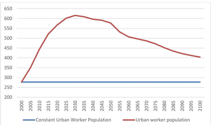
The first exogenous variable is urban worker population. According to the conclusions of
Chapter 5, the worker population has a profound influence on land prices. Because we focus
consideration. In particular, we assume that the rural and urban areas have the same age
structure. Thus, the urban worker population can be calculated by the total worker population
and the rate of urbanization (the projection data of the UN on these two factors can be seen in
the survey chapter (Chapter 3)). Here, because there is no projection of urbanization rate from
2050 to 2100, we assume this rate would rise from 77 percent (the UN projection of 2050) to
80 percent with a uniform speed during this period. Then, the calculated urban worker
population from 2000 to 2100 is shown in Fig. 7-1.
From Fig. 7-1, we can see that the urban worker population of China rises from 2000 to 2030
and then declines until the end of this century. The rising of the population is caused by rapid
urbanization, while the decline is driven by the decline of fertility rate that is lower than the
replacement level. As shown in Fig. 7-1, the population peaks in 2030 and then drops off.
Although the decline will last for a long time, the range of this decline is modest compared
[image:16.595.121.477.364.557.2]with that of the rising before (relying on the UN projections).
Figure 7-1 Urban Worker Population Projection
Note: source from the projection data of the UN. From 2050 to 2100, the projected
urbanization rate is assumed to increase from 77 percent to 80 percent.
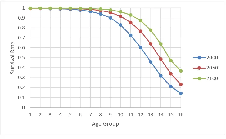
The second exogenous variable is the longevity of households. This variable is denoted by
the survival rates of different age groups. According to the dataset of the UN, the projection
of longevity in China will increase from 2000 to 2100. This increase has been shown in Fig.
7-2 by presenting the survival rates of different age groups in 2000, 2050 and 2100. As we
can see, the survival rates in 2100 is higher than those in the 2050 and 2000, and this higher
survival rate implies a higher longevity.
200 250 300 350 400 450 500 550 600 650
2000 2005 2010 2015 2020 2025 2030 2035 2040 2045 2050 2055 2060 2065 2070 2075 2080 2085 2090 2095 2100
M
il
li
o
Notice that the survival rates of age group 16 increase from 14 percent to 37 percent within
the period, there could be a number of households aged more than 99. For these households,
their behaviours are not modelled. Here, we assume that they are taken care of by the health
care centre that owned by the government. The funding of this centre could come from the
housing assets of these households. Recall that the houses and land of households who are
aged more than 99 are assumed to be collected by the government, the operation of this
[image:17.595.116.480.227.451.2]centre is funded by selling these assets.
Figure 7-2 Survival Rates of Age Groups in 2000, 2050 and 2100
Note: source from the projection data of the UN.
The last exogenous variable is the age structure of households. This variable is independent
only when the migration is significant. In this case, the age structure cannot be determined by
the fertility rates and survival rates. Specifically, we denote this variable by the ratio of the
population of age group 𝑖𝑖and total worker population. The selected age structures in 2000,
2050 and 2100 are shown in Fig. 7-3. In this figure, we can see a significant population
ageing since the share of the elderly is rising along with time. Besides, the shares of age
groups are not smooth. For example, in 2050, the share of the ninth age group (that is, those
aged between 60 and 64) is substantially higher than the other age groups and this spike10
10 The age structure spike is due to a baby boom that happens during 1986 and 1990. The birth rate during this
period is higher than both the before and after. Along with the time, this baby boom will reach age 60-64 (group 9) in 2050, forming the spike as shown in the figure.
0 0.1 0.2 0.3 0.4 0.5 0.6 0.7 0.8 0.9 1
1 2 3 4 5 6 7 8 9 10 11 12 13 14 15 16
Su
rv
iv
a
l Ra
te
Age Group
may impact on the land price. These impacts of different age structures will be discussed in
[image:18.595.109.489.124.343.2]section 5.
Figure 7-3 Age Structures in 2000, 2050 and 2100
Note: source from the projection data of the UN.
0 0.02 0.04 0.06 0.08 0.1 0.12 0.14 0.16 0.18
1 2 3 4 5 6 7 8 9 10 11 12 13 14 15 16
Ra
ti
o
s
Age Group
Quantitative Results
A. Fitting Historical Data
Before the projection and simulation, we want to know if our model could provide insights
into the land price dynamics in China. In particular, we check this question by fitting our
model to the historical data.
Here, this historical data is the quotient of total transaction price and land area purchased by
the real estate development enterprises. Thus, it is an averaged contract price. We use this
total transaction price instead of the total expenditure because: 1) according to the National
Bureau of Statistics (NBS) of China, the transaction price and the land area have the same
statistical calibre11; 2) the total expenditure includes taxes, land requisition compensation,
and accounting rules12, and these factors have not been considered in our model. Therefore,
we will study the transaction price only.
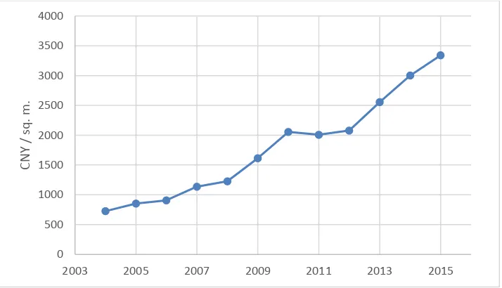
This transaction price data is shown in Fig. 7-4. From 2004 to 2015, the land price in nominal
terms rises from 726 to 3341 CNY/sq. m., amounting to an increase of 3.6 times. The
demography itself may not form such a rapid rise, and, at least, the increase of per capita
income during this period should be taken into consideration. Nevertheless, when fitting the
historical data, we want to exclude the effect of income on the land price and focus on the
effect of demographic changes. The reason is that, in the simulations, the expectations of
future income can significantly affect the current growth rates of land price. However,
forecasting income has proved to be hard in practice, and thus beyond the scope of this thesis.
To exclude the effect of income, we take the assumption that, when income increase by one
percent, the land price will also increase by one percent (the elasticity is one), and this
assumption is based on the following reasons. Theoretically, using the method presented in
the appendix of Chapter 5, the trend growth rate of land price can be expressed as:
𝑔𝑔𝑝𝑝𝑙𝑙,𝑡𝑡 =𝑔𝑔𝑦𝑦,𝑡𝑡+𝑔𝑔𝑁𝑁,𝑡𝑡− 𝑔𝑔𝐿𝐿,𝑡𝑡 (7-18)
Here, the variables 𝑔𝑔𝑝𝑝𝑙𝑙,𝑡𝑡, 𝑔𝑔𝑦𝑦,𝑡𝑡,𝑔𝑔𝑁𝑁,𝑡𝑡 and 𝑔𝑔𝐿𝐿,𝑡𝑡 denote the trend growth rates of land price, per
capita income, urban worker population and land restrictions. This equation implies that our
assumption will hold true when the trend in land prices net of the rate of growth in per capita
GDP is considered. In addition, the empirical studies, such as Takáts (2012) and Wang and
Zhang (2014), have suggested that the one percent increase in income would correspond with
one percent increase in house price. As an important constituent of housing, we suppose that
it is also the case for the land price. If true, we can subtract the income growth rate from the
[image:20.595.120.477.187.392.2]land price growth rate to obtain the requisite data13.
Figure 7-4 Historical Land Price of China (2004-2015)
Note: source from the database of National Bureau of Statistics of China and author
calculation.
The fitted result is shown in Fig. 7-5. The blue line denotes the cumulative growth of land
price that excluded the effect of income as discussed above. Comparing with the land price in
Fig. 7-4, this cumulative growth is moderate. In Fig. 7-5, the red line is the baseline
projection of our model. Here, the results from the baseline projection is yearly averaged so
as to fit the historical data. In this figure, although the projection cannot capture all of the
fluctuations in the land price, these two matches well in trend from 2005 to 2015. This result
suggests that the effects of demographic changes are important in forming the land price, and
our model would provide clues in forecasting these effects. Nevertheless, because the data
length of this fitting is relatively short, these conclusions may need further examination as
more data is made available.
In addition, the fitting result also implies that the bulk of land price dynamics in China could
be explained from the perspective of income and demography. This conclusion suggests that
13 Because both the land price and the income are in nominal terms and have inflation included, the subtraction
of their growth rates would exclude the inflation.
0 500 1000 1500 2000 2500 3000 3500 4000
2003 2005 2007 2009 2011 2013 2015
C
N
Y
/
s
q
. m
there could be no bubble in the housing prices of China in the current stage as the findings in
the empirical studies14. Here, the rising per capita income has contributed the most to the rise
in the land price, and the demography is a secondary factor. Yet, the demographic changes
are more predictable and stable. Thus, in the following section, we will focus on the impact
of the demographic changes on the land price and omit the influences from other factors.
[image:21.595.114.480.206.421.2]Also, in all the results below, the land price and its dynamics are calculated in real terms.
Figure 7-5 Fitting the Historical Data (excluded the effect of income, 2005-2015)
Source: author calculation.
14 See, for example, Ren, Xiong, and Yuan (2012), Shen (2012), and Deng, Girardin, and Joyeux (2016).
0.6 0.7 0.8 0.9 1 1.1 1.2
2005 2006 2007 2008 2009 2010 2011 2012 2013 2014 2015
B. Baseline Projection15
Our main results of the baseline projection can be represented by the cumulative growth of
urban land price as shown in Fig. 7-6. In this figure, the dynamics of land prices from 2000 to
2100 can be divided into three stages. In the first stage, the positive effect of demographic
changes will dominate from 2000 and last until 2035. After that, the second stage lasts from
2035 to 2055. Within this period, the effect of demographic changes on land price is close to
zero. This stable period implies there may not be a sharp turning point in the price dynamics.
In the last stage starts from 2055, the impacts from demographic changes turn to negative and
will last until the end of this century. However, the downward effect is not symmetric
compared with the rising in the beginning of this century. By 2100, our simulation indicates
[image:22.595.110.485.310.528.2]that the cumulative growth would be nearly the same as that of 2015.
Figure 7-6 Baseline Projection: Cumulative Growth of Urban Land Price (2000-2100)
Source: author calculation.
The growth rates of urban land price from 2000 to 2100, which is shown in Fig. 7-7, can
provide additional information from another angle. As we can see, the rapid rising land price
has been cooling down, implying the booming of land price may not reoccur to the same
extent. This result corresponds well with other empirical studies (see Wu, Gyourko, and Deng
(2016)). Along with this cooling down, the growth rates will turn to negative between 2050
and 2055. After 2055, although the growth rates could be positive around 2070 (see Fig 7-7),
15 The detail settings of the simulation will be shown in Appendix.
0 5 10 15 20 25 30 35 40
2000 2005 2010 2015 2020 2025 2030 2035 2040 2045 2050 2055 2060 2065 2070 2075 2080 2085 2090 2095 2100
P
er
cen
the overall growth rate is negative. Nevertheless, the fall can hardly be described as a
[image:23.595.113.485.123.359.2]meltdown because the decline is moderate.
Figure 7-7 Baseline Projection: Growth Rates of Urban Land Price (2000-2100)
Source: author calculation.
Here, we want to explain three features implied in this baseline projection. The first feature is
the asymmetry of the rising and the declining prices of urban land, and we will argue that this
asymmetry is due to the urbanization. In 2000, the urbanization rate in China is 36 percent;
however, according to the forecasts of the UN, this ratio would be 77 percent by 2050. The
fast-rising urbanization continues to provide labour to the urban area, supporting the urban
economic development and the corresponding rise in the price of land. Meanwhile, the rising
urbanization ratio is unlikely to be reversed given the worldwide experience. Thus, the
predicted decline will not be as dramatic as the rising (see Fig. 7-6, 7-7). In addition, we
assume that the urbanization ratio continues to rise after 2050, and a conservative estimate of
this ratio would be 80 percent by 2100, and our Baseline Projection above is based on this
assumption.
Second, the cumulative growth of the land price in Fig. 7-6 is much lower than that of the
worker population. Note that the worker population determines the trend of land price16
16 We only consider the demographic factors in the baseline projection, and the accurate trend formed by worker
population is 𝑔𝑔𝑝𝑝𝑙𝑙 =1−𝜇𝜇𝑐𝑐−𝜇𝜇𝑙𝑙
1−𝜇𝜇𝑐𝑐 𝑔𝑔𝑛𝑛. When the parameter 𝜇𝜇𝑙𝑙 is small, the trend of land price would be approximately
the same as the trend of worker population.
-6 -4 -2 0 2 4 6 8 10 12
2000 2005 2010 2015 2020 2025 2030 2035 2040 2045 2050 2055 2060 2065 2070 2075 2080 2085 2090 2095 2100
P
er
cen
according to Eq. 7-18, this result indicates that the projection is lower than the trend. Why is
that? The reason lies in the assumption that households have perfect foresight. Thus, the
households foresee that the worker population will decline in the future and so will the land
price. This mechanism can be explained by the Euler Equation of households as follows:
𝑝𝑝𝑙𝑙,𝑡𝑡 = 𝛽𝛽𝐸𝐸𝑡𝑡�𝑝𝑝𝑙𝑙,1+𝑡𝑡
𝑐𝑐𝑡𝑡,𝑖𝑖
𝑐𝑐𝑡𝑡+1,𝑖𝑖+1
𝜋𝜋1+𝑡𝑡,1+𝑖𝑖
𝜋𝜋𝑡𝑡,𝑖𝑖 �
+𝑗𝑗𝑙𝑙𝑐𝑐𝑖𝑖,𝑡𝑡
𝑙𝑙𝑖𝑖,𝑡𝑡
(7-19)
According to this equation, when a lower future land price, 𝑝𝑝𝑙𝑙,1+𝑡𝑡, is predicted, the current land price, 𝑝𝑝𝑙𝑙,𝑡𝑡, will also decline. Therefore, the rising of the land price will not reach the same extent as indicated by the worker population. This mechanism will prevent the prices
from suddenly spiking.
Third, the dynamics of the worker population suggests that the prices would tend to decline
from 2035. However, our simulation indicates a stable period from 2035 to 2055. How does
this difference arise? Here, we argue that this difference comes from the movement of age
structure of households. Specifically, if the age structure is more / less centred, the aggregate
land demand will be higher / lower, and thus the land price will tend to rise / decline17. After
2035, the fertility rate decline will drag down the worker population; nevertheless, because of
the fall in the share of the youth population, the age structure would be more centred (as an
example, see the red line in Fig. 7-3), forming an upward force supporting the land price.
Consequently, the stable period of land prices comes from the overall effect of these two
forces.
17 This is one of the conclusions of the section 5 of this chapter. In that section, a detailed discussion on the
C. Counterfactual Simulations
In this study, the demographic changes are described by 1) worker population, 2) survival
rates (longevity), and 3) age structures. The overall effect on the land price dynamics is
caused by all the three factors. Nevertheless, the effect of each of the three factors is missing
in the baseline projection above, and this question is important for the further understanding
of the influence of an aging population. To this end, following Muto, Oda, and Sudo (2016),
we conduct counterfactual simulations to check the effects of these three factors respectively.
First, we assume that the worker population stays the same during our simulation, and the
other settings are the same as in the baseline projection. In this circumstance, the worker
population would be lower than that of the baseline projection (see Fig. 7-8). The
[image:25.595.117.478.322.536.2]consequences of this setting on the urban land price are shown in Fig. 7-9 and 7-10.
Figure 7-8 Constant Worker Population (2000-2100)
Source: author calculation.
Comparing with the baseline projection, we can see that a lower worker population will
greatly lower the cumulative growth of the urban land price (see Fig. 7-9). This result
suggests that the growth of urban worker population is the dominant demographic factor
supporting the rising of the urban land price in the baseline projection.
Second, if we suppose that the survival rates of households are constants from 2000 (see Fig.
7-2), the counterfactual simulation results are shown in Fig. 7-11 and 7-12. As we can see,
this change has little impacts on the growth rates from 2000 to 2100. Recall that we have
200 250 300 350 400 450 500 550 600 650
2000 2005 2010 2015 2020 2025 2030 2035 2040 2045 2050 2055 2060 2065 2070 2075 2080 2085 2090 2095 2100
shown that the changes in longevity have significant effect on land prices in Chapter 5, then
[image:26.595.110.487.157.368.2]why the lower longevity here has little influence on the growth rates?
Figure 7-9 Counterfactual Simulation with Lower Worker Population: Cumulative Growth of
the Urban Land Price (2000-2100)
[image:26.595.112.484.447.681.2]Source: author calculation.
Figure 7-10 Counterfactual Simulation with Lower Worker Population: Growth Rates of the
Urban Land Price (2000-2100)
Source: author calculation.
-10 -5 0 5 10 15 20 25 30 35 40
2000 2005 2010 2015 2020 2025 2030 2035 2040 2045 2050 2055 2060 2065 2070 2075 2080 2085 2090 2095 2100
P
er
cen
t
Counterfactual Simulation Baseline Projection
-6 -4 -2 0 2 4 6 8 10 12
2000 2005 2010 2015 2020 2025 2030 2035 2040 2045 2050 2055 2060 2065 2070 2075 2080 2085 2090 2095 2100
P
er
cen
t
The first reason is that, because of perfect foresight, the bulk of the effect of survival rate
changes happen before 2000. Thus, for the periods of our concern, the impacts have been
absorbed beforehand. Second, the survival rate changes here have different consequences
compared with that of the Chapter 5. When we change the survival rates in Chapter 5, the
corresponding households’ age structure changes. However, in this chapter, the age structure
is viewed as an independent exogenous variable because of migration. Therefore, the effects
of age structure changes are isolated from that of the longevity changes, so the impacts of the
[image:27.595.113.484.248.467.2]longevity changes are weakened.
Figure 7-11 Counterfactual Simulation with Lower Longevity: Cumulative Growth of the
Urban Land Price (2000-2100)
Source: author calculation.
0 5 10 15 20 25 30 35 40
2000 2005 2010 2015 2020 2025 2030 2035 2040 2045 2050 2055 2060 2065 2070 2075 2080 2085 2090 2095 2100
P
er
cen
t
Counterfactual Simulation Baseline Projection
-6 -4 -2 0 2 4 6 8 10 12
2000 2005 2010 2015 2020 2025 2030 2035 2040 2045 2050 2055 2060 2065 2070 2075 2080 2085 2090 2095 2100
P
er
cen
t
Figure 7-12 Counterfactual Simulation with Lower Longevity: Growth Rates of the Urban
Land Price (2000-2100)
[image:28.595.113.483.144.362.2]Source: author calculation.
Figure 7-13 Counterfactual Simulation with Younger Age Structure: Cumulative Growth of
the Urban Land Price (2000-2100)
[image:28.595.112.485.444.673.2]Source: author calculation.
Figure 7-14 Counterfactual Simulation with Younger Age Structure: Growth Rates of the
Urban Land Price (2000-2100)
Source: author calculation.
0 10 20 30 40 50 60
2000 2005 2010 2015 2020 2025 2030 2035 2040 2045 2050 2055 2060 2065 2070 2075 2080 2085 2090 2095 2100
P
er
cen
t
Counterfactual Simulation Baseline Projection
-6 -4 -2 0 2 4 6 8 10 12
2000 2005 2010 2015 2020 2025 2030 2035 2040 2045 2050 2055 2060 2065 2070 2075 2080 2085 2090 2095 2100
P
er
cen
t
Regarding the age structure, when it is held constant to that of 2000 during the simulation, the
results comparing with the baseline projection are shown in Fig. 7-13 and 7-14. Note that the
age structure in 2000 is the youngest in this century (see Fig. 7-3), this comparison could tell
us the effect of a younger age structure on the land price dynamics. As shown in Fig. 7-13,
because of a younger age structure, the growth rates of land price are higher than that of the
baseline projection in most of the periods. This result suggests that the age structure changes
from 2000 to 2100 will significantly depress the growth rates of land price in urban China.
The key findings of the quantitative study in this section can be summarized as follows. First,
the historical land price dynamics in China can be explained from the perspective of income
and demography. Second, the on-going aging population in China will drag down the land
price during the second half of this century, but will not force the dynamics into a crash.
Third, the demographic factors have divergent effects on the land price. Specifically, the
rising of the urban worker population is supporting the price in general, while the age
Age Structure and Land Demand
Within the three exogenous variables, the effects of worker population and longevity on land
prices have been discussed in detail in the previous chapters. Nonetheless, the effect of age
structure changes has not been discussed. Since this factor can only be isolated when
migration is significant in the demographic changes, this discussion has to be located here
instead of the previous chapters. Then, how does age structure affect land prices?
The key to answer the above question is noting the difference in demand for land by different
age groups. As shown in Fig. 7-15, the land demand in our simulation varies across the age
groups. In general, the land demand of the middle age groups is higher, and that of the youth
and elderly is lower. This result corresponds well with the life cycle hypothesis about
households saving behaviour. When age structure changes, the total land demand will change
accordingly. For example, if more of the households are in the age group nine / sixteen, the
total land demand will be higher / lower. Note that the land supply is fixed in our simulation,
ceteris paribus, the changes in land demand will determine the price dynamics. Consequently,
[image:30.595.114.480.412.628.2]the land price will rise / decline.
Figure 7-15 De-trended Per Capita Land Demand of Different Age Groups (Baseline
Projection in 2000)
Source: author calculation.
The mechanism above provides a brief explanation about how changes in the age structure
affect land prices. In fact, the empirical studies, such as Mankiw and Weil (1989), have
adopted this mechanism in predicting the house prices. They used a survey data of house
0 0.2 0.4 0.6 0.8 1 1.2 1.4 1.6
1 2 3 4 5 6 7 8 9 10 11 12 13 14 15 16
la
nd de
m
a
nd
owned per capita by age to forecast the house price dynamics according to the predicted age
structure changes. However, the model in this chapter will show that the demand is
conditional on and subject to demographic changes. Therefore, the historical survey data
cannot provide accurate predictions about the demand in the future.
To begin with, the growth rate of worker population will change the land owned per capita.
For instance, when the worker population keeps growing, the land owned per capita would
tend to decline because the land supply is fixed in our assumptions. Furthermore, even if we
only consider the de-trended value of the per capita owned land, this value will also change in
different circumstances. For example, the de-trended per capita owned land of the baseline
projection in different periods is shown in Fig. 7-16. As we can see, this land demand by age
groups varies across the periods. In 2000, the households have the highest per capita land
demand among all the periods. After that, this demand decreases along with time until 2060.
[image:31.595.114.482.364.581.2]From 2060 to 2100, this land demand stays in a stable state.
Figure 7-16 De-trended Per Capita Land Demand of the Baseline Projection
Source: author calculation.
Next, we will study the specific mechanisms that how the demand of land is affected by the
demographic changes. First, we argue that a higher / lower growth rate of worker population
will indicate a higher / lower land demand of households. To illustrate, we calculate the per
capita land demand of households when the worker population growth rates are 0.2, 0, and
-0.1 respectively, and the results are shown in Fig. 7-17. As we can see, the results correspond
well with our argument above. The direct reason is that a higher land price is predicted by the
0 0.2 0.4 0.6 0.8 1 1.2 1.4 1.6
1 2 3 4 5 6 7 8 9 10 11 12 13 14 15 16
la
nd de
m
a
nd
age groups
households in the next period. When the worker population growth rate is higher, the price of
land would tend to rise according to Eq. 7-18. Thus, purchasing land becomes a better saving
[image:32.595.116.480.142.363.2]method, and consequently, the land demand of households rises.
Figure 7-17 De-trended Per Capita Land Demand for three rates of growth of Worker
Population
Note: the calculation is based on hypothetical worker population growth rates, and the other
settings are the same as the baseline projection in 2000.
Figure 7-18 De-trended Per Capita Land Demand of Various Longevity
Note: the lower / higher longevity uses the survival rates in 2000 / 2100, other settings are the
same as in the baseline projection in 2000.
0 0.2 0.4 0.6 0.8 1 1.2 1.4
1 2 3 4 5 6 7 8 9 10 11 12 13 14 15 16
la
nd de
m
a
nd
age groups
n=0.2 n=0 n=-0.1
0 0.2 0.4 0.6 0.8 1 1.2 1.4 1.6
1 2 3 4 5 6 7 8 9 10 11 12 13 14 15 16
la
nd de
m
a
nd
age groups
[image:32.595.117.478.474.689.2]Second, we argue that a higher / lower longevity suggests a higher / lower land demand of
households. To test this argument, we simulate the land demand of households by changing
the longevity only, and the results are shown in Figure 7-18. As we can see, the results are
supportive of our argument above. The mechanism of this movement can also be explained
from the perspective of households’ behaviour. Note that a higher longevity indicates more
savings are required to support the consumption, the land demand will increase
correspondingly because land ownership is the only means of saving in the model (as it is one
[image:33.595.92.509.258.303.2]of the major sources of saving in reality).
Figure 7-19 The Effect Channel from Age Structure Changes to Per capita Land Demand
Figure 7-20 De-trended Per Capita Land Demand: Age Structure Changes
Note: the calculation is based on hypothetical age structures, the detail will be listed in
Appendix. The other settings are the same as the baseline projection in 2000.
Lastly, the per capita land demand will vary when age structure changes. Specifically, when
the age structure is more centred, the per capita owned land will be lower ceteris paribus. The
mechanism driving the differences is shown in Fig. 7-19. In the first step, the changes of age
structure will affect the total land demand of households as discussed above. Supposing the
age structure is more centred, then the total land demand will rise. Then, because of the rising
of the land demand, the land price will rise accordingly. Finally, the raised land price will
0 0.2 0.4 0.6 0.8 1 1.2 1.4
1 2 3 4 5 6 7 8 9 10 11 12 13 14 15 16
la
nd de
m
a
nd
age groups
less centred age structure more centred age structure
Age Structure
Total Land
Demand Land Price
[image:33.595.114.480.350.574.2]depress the per capita land demand. When we face a less centred age structure, the effects are
Conclusion
The literature on the drivers for land prices suggests that demography is an important
factor18. However, the forecasting of the land price dynamics has long been long reliant on
the data-driven methods instead of theoretical models. In this study, we want to fill this gap
by forecasting the effects on land price using the case of China. Choosing China also has
significant practical meaning because China is experiencing a strongly aging population,
which would, according to the life-cycle hypothesis, drag down land prices. Since the land
price has profound influences on the households’ wealth and macroeconomic stability, our
forecasting should answer the question that whether the price of land will collapse due to the
aging of the population?
To answer this question, this chapter develops an OLG model with multiple generations, and
uses simulations to forecast the land price dynamics using parameters for the model from
urban China. To check if this simulation could provide clues to the future land price, we fit
the historical data from 2005 to 2015 using the projections. The reasonable fit of the
historical data to the results from the simulation indicates that the rapid rise in land price over
the past decade can be explained from the perspective of income and demography. Although
demography plays a secondary role in driving land prices, it is the more predictable and
stable factor compared to GDP.
Next, we present the baseline projection of land price dynamics from 2000 to 2100. The
result shows that the aging of the population on its own will not lead to a collapse in land
prices. Specifically, although the land prices have been cooling down, demographic changes
will continue to raise land prices until 2035, following which they stabilise until 2055. After
that, the impact on land prices from demographic changes are negative, meaning that land
prices decline until the end of this century. However, the decline of land price is predicted to
be moderate and very different to the pattern during the upswing.
The forecast above is based on three exogenous variables used in this simulation: 1) worker
population, 2) longevity, and 3) age structure. This chapter also examined their effects using
counterfactual simulations. In particular, from 2000 to 2100, the overall effect of worker
population on land price dynamics is positive, and the bulk of the rise is caused by the
increase of worker population. In contrast, the overall effect of the aging age structure is
negative from 2000 to 2100, which corresponds well with the Life-Cycle Hypothesis. Here,
we want to emphasize that the age structure changes cannot represent the whole aging
population process on its own. Instead, as illustrated in the context, the age structure is only a
part of it and could be viewed as an independent variable only when the migration is
significant. Lastly, the effect of longevity is not significant from 2000 to 2100 because the
bulk of its effects are absorbed by 1) the price changes beforehand, and 2) the effect of age
structure changes.
Besides an analysis of these issues, we discussed the drawbacks of the forecast when
conducted by historical survey data. We argue that this kind of forecast depends on the per
capita land owned of households; however, this land demand is conditional and will vary in
different circumstances. In fact, our simulations suggest that all the three exogenous
demographic factors can change the demand significantly. Thus, the data-driven methods
may have limited capacity in forecasting the land price when the demographic changes are
substantial.
Several caveats to the conclusions drawn above are in order here. These include the fact that
the OLG model has been used for the simulations, in which the households are assumed to be
homogenous in each and every age group. Further research may consider the heterogeneity
agent models for improvements. The other issue regards with the data of land price that we
adopt. We care about the average contract price of the land in this study; however, the real
payment of the building business could also include the taxes and the compensation to
households for land acquisition. Thus, the real payment could be much higher than the
contract price, and these extra payments are left for further studies.
In sum, this chapter contributes the literature that studying the effect of aging by analysing
the case of China. The results suggest that the demography has profound impact on the land
prices, but a meltdown is unlike to happen in China. These results could also be of practical