Patchwise Mapping Method for Solving Elliptic Boundary Value Problems Containing Multiple Singularities

http://www.scirp.org/journal/jamp ISSN Online: 2327-4379

ISSN Print: 2327-4352

DOI: 10.4236/jamp.2019.77107 Jul. 29, 2019 1572 Journal of Applied Mathematics and Physics

Patchwise Mapping Method for Solving Elliptic

Boundary Value Problems Containing Multiple

Singularities

Hyunju Kim

Department of Mathematics, North Greenville University, Tigerville, SC, USA

Abstract

In the paper [1], the geometrical mapping techniques based on Non-Uniform Rational B-Spline (NURBS) were introduced to solve an elliptic boundary value problem containing a singularity. In the mapping techniques, the in-verse function of the NURBS geometrical mapping generates singular func-tions as well as smooth funcfunc-tions by an unconventional choice of control points. It means that the push-forward of the NURBS geometrical mapping that generates singular functions, becomes a piecewise smooth function. However, the mapping method proposed is not able to catch singularities emerging at multiple locations in a domain. Thus, we design the geometrical mapping that generates singular functions for each singular zone in the phys-ical domain. In the design of the geometrphys-ical mapping, we should consider the design of control points on the interface between/among patches so that global basis functions are in 0

C space. Also, we modify the B-spline func-tions whose supports include the interface between/among them. We put the idea in practice by solving elliptic boundary value problems containing mul-tiple singularities.

Keywords

Mapping Method, Non-Uniform Rational B-Spline (NURBS), Galerkin Approximation, Isogeometric Analysis, Multiple Singularities

1. Introduction

It has been introduced to solve multiple crack problems by using various nu-merical methods. First, converting the multiple crack problems into Fredholm integral equation using two elementary solutions was introduced in [2]. A

nu-How to cite this paper: Kim, H. (2019) Patchwise Mapping Method for Solving Elliptic Boundary Value Problems Con-taining Multiple Singularities. Journal of Applied Mathematics and Physics, 7, 1572-1598.

https://doi.org/10.4236/jamp.2019.77107

Received: February 5, 2019 Accepted: July 26, 2019 Published: July 29, 2019

Copyright © 2019 by author(s) and Scientific Research Publishing Inc. This work is licensed under the Creative Commons Attribution International License (CC BY 4.0).

DOI: 10.4236/jamp.2019.77107 1573 Journal of Applied Mathematics and Physics

merical method by using both Fredholm integral equation method and the weighted residual method was introduced in [3]. Numerical methods based on Galerkin approximation such as the finite element methods, boundary element methods, and meshless method were also applied to solve them [3]-[10].

In this paper, we solve the elliptic boundary value problems with multiple singularities based on the mapping method [1]. But, the mapping technique proposed is not able to catch singularities emerging at multiple locations in a domain. In order to resolve the drawback, we introduced the enriched Isogeo-metric Analysis (IGA) in [11]. In the paper [11], we approximate the solution on the small circular zone centered at the crack tip or point singularity by enriching the finite approximation space generated by the singular mapping introduced in the mapping method. However, it is hard to evaluate the inverse functions of the singular mapping, and the NURBS mapping so that tracking the domains of in-tegrals whose integrand is involved both B-spline function from the singular mapping and NURBS function from the NURBS geometrical mapping, is an ad-ditional work. Also, the conad-ditional number of the stiffness matrix could be an issue for the enriched IGA. In order to alleviate these problems, we design the geometrical map having multiple singularities by using the singular mappings only. To do that, we divide the physical domain into multiple patches which may have a singularity for each, and then design the geometrical maps by the map-ping methods for each patch having a singularity. Here, we consider the design of control points on the interface between/among patches. Because this is related to the smoothness of the global basis functions. Also, we modify the B-spline functions whose supports include the interface between/among them due to the compatibility condition. In this paper, the potential of the mapping method proposed with multiple patches regarding to handling the multiple fatigue-cracks propagation in various types of plate will be shown by solving the elliptic boun-dary value problems with multiple singularities or cracks.

In Section 1 and 2, we briefly review definitions and terminologies that are used throughout this paper. We follow those in the book [12], and we thus refer to these texts for details. And then we introduce the mapping method that gene-rates singular functions by using B-spline or NURBS in Section 3. In Section 4, we introduced the patchwise mapping method by solving elliptic boundary value problems containing multiple singularities. Finally, the conclusions is in Section 5.

2. Nomenclature

In this section, we introduce B-spline, NURBS, and design geometrical map-pings referring to [12].

2.1.

B

-Splines

A knot vector U =

{

u u1, 2,,um

}

is a nondecreasing sequence of real numbers

DOI: 10.4236/jamp.2019.77107 1574 Journal of Applied Mathematics and Physics

1 p1 p 2 m p 1 m p m,

u ==u ₊ <u ₊ ≤≤u _{− −} <u ₋ ==u in which the first and the last p+1 knots are repeated.

The B-spline functions Bi k,

( )

ξ of order k= +p 1 corresponding to the

knot vector U =

{

u u1, 2,,um

}

are piecewise polynomials of degree p which

are constructed recursively by the Cox-de Boor recursion formula:

( )

( )

( )

( )

1 ,1

, , 1 1, 1

1 1

1 if ,

0 otherwise,

, i i

i

i i k

i k i k i k

i k i i k i

u u

B

u u

B B B

u u u u

ξ ξ

ξ ξ

ξ ξ ξ

+ +

− + −

+ − + +

≤ < 

=  

− −

= +

− −

for 1≤ ≤i

(

m−k

)

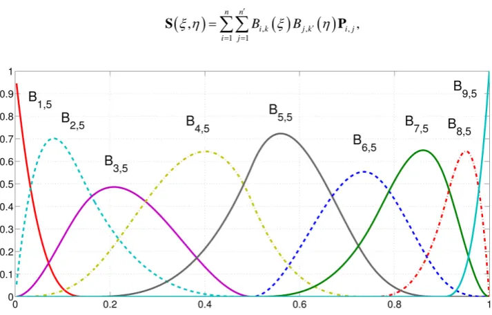
For example, the piecewise quadratic polynomial B-spline

functions Bi,5

( )

ξ corresponding to the open knot vector

{

0, 0, 0, 0, 0, 0.15, 0.5, 0.75, 0.9,1,1,1,1,1

}

U=

are depicted in Figure 1.

The B-spline functions are useful in design as well as finite element analysis because they have the following properties: variation diminishing, convex hull, non-negativity, piecewise polynomial, compact support, and partition of unity.

A B-spline curve is defined as follows:

( )

,

( )

1

, n

i k i i

B

ξ

ξ

=

=

∑

C P

where n= −m k and

{ }

P_i are control points that make B-spline functions draw a desired curve as shown in Figure 2(a).

Let Uη =

{

v1,,vm′

}

be an open knot vector and let pη and k′ = pη +1,

respectively, be the polynomial degree and order of B-spline functions Bj k, ′

( )

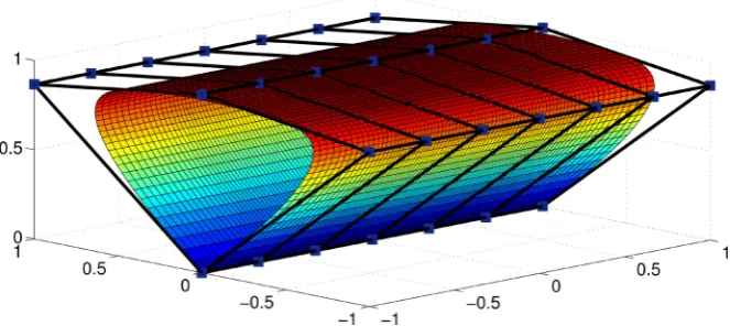
η .

Then a B-spline surface is defined by

(

)

,

( )

,

( )

,

1 1

, ,

n n

i k j k i j

i j

B B

ξ η ′ ξ ′ η = =

=

∑∑

[image:3.595.182.539.461.689.2]

S P

Figure 1.B-spline functions Bi,5

( )

ξ , i=1, 2,,9 of order k=5 corresponding to the knot

[image:4.595.173.540.65.458.2]

DOI: 10.4236/jamp.2019.77107 1575 Journal of Applied Mathematics and Physics

Figure 2. (a) B-spline curve and control points on the open knot vector

{

0,0,0,0.15,0.42,0.76,0.76,0.91,0.91,1,1,1

}

. (b) B-spline basis functions corresponding to the

B-spline curve shown in (a). (a) B-spline curve and control points; (b) B-spline basis functions.

where n′=m′−k′ and P_{i j,} are control points that make a bidirectional control net as shown in Figure 2(b).

2.2. Nonuniform Rational

B

-Spline (NURBS)

In this section, we review the non-uniform rational B-splines (NURBS), NURBS curve and surface, and primary properties of NURBS.

2.2.1. NURBS Curve

A pth-degree NURBS curve is defined by

( )

( )

( )

, 1

, 1

, n

i k i i i

n

i k i i

B w

a b

B w

ξ

ξ ξ

ξ

= =

=

∑

≤ ≤

∑

P C

(1)

DOI: 10.4236/jamp.2019.77107 1576 Journal of Applied Mathematics and Physics

and the

{

Bi k,

( )

ξ

}

are the pth-degree B-spline basis functions defined on the

nonperiodic (and non-uniform) knot vector

2

1 1

, , , p , , m k, , , .

p p

U a a u + u − b b

+ +     =        

We assume that a=0,b=1, and wi>0 for all i. Setting

( )

( )

( )

, , , 1

i k i

i k n

j k j

j B w R B w ξ ξ ξ = =

∑

(2)

allows us to rewrite Equation (1) in the form

( )

,

( )

1 n

i k i i R

ξ

ξ

= =

∑

C P (3) The

{

Ri k,

( )

ξ

}

are the rational basis functions; they are piecewise rational

functions on ξ∈

[ ]

0,1.

2.2.2. NURBS Surface

A NURBS surface of degree p_ξ in the ξ direction and degree p_η in the

η

direction is a bivariate vector-valued piecewise rational function of the form

(

)

( )

( )

( )

, , , , 1 1 , , , 1 1 ( )

, , 0 , 1

n n

i k j k i j i j i j

n n

i k j k i j i j

B B w

B B w

ξ η

ξ η ξ η

ξ η ′ ′ = = ′ ′ = = =

∑∑

≤ ≤

∑∑

P S (4)

The

{ }

Pi j, form a bidirectional control net, the

{ }

wi j, are the weights, and

the

{

Bi k,

( )

ξ

}

and

{ }

Bj k, ′ are the nonrational B-spline basis functions defined

on the knot vectors

( ) 

1 1

1 1

0, , 0 , _p , , ,1, ,1 ,

m p p p

U u_ξ u

ξ ξ ξ + − + + +     =           ( )  1 1 1 1

0, , 0 , _p , , ,1, ,1 .

m p p p

V v v

ξ η η η + ′− + + +     =          

Introducing the piecewise rational basis functions

(

)

( )

( )

( )

( )

, , , , , , , 1 1

, i k j k i j

i j n n

s k t k s t

s t

B B w

R

B N w

ξ η ξ η ξ η ′ ′ ′ = = =

∑∑

the surface Equation (4) can be written as

(

)

,

(

)

,

1 0

, , .

n n

i j i j

i j

R

ξ η ′ ξ η = =

=

∑∑

S P

An example of the NURBS surface is shown in Figure 3.

2.3. Weak Solution in Sobolev Space

[image:6.595.209.541.74.222.2]

DOI: 10.4236/jamp.2019.77107 1577 Journal of Applied Mathematics and Physics

Figure 3. An example of B-spline surface with control net in three dimensional space.

to consist of all those functions φ which, together with all their partial

deriva-tives

(

1

)

1 d d

α α

α_{φ φ}

∂ = ∂ _∂ _{of orders} α =α₁++α_d ≤m, are continuous on

Ω. A function

φ

_∈m

( )

_{Ω is said to be a }m-function. If _Ψ is a function defined on Ω_{, we define the support of} Ψ _as

( )

{

}

suppΨ = x∈ Ω Ψ| x ≠0 .

For an integer k≥0, we also use the usual Sobolev space denoted by

( )

k

H Ω . For u∈Hk

( )

Ω , the norm and the semi-norm, respectively, are

( )

{

}

( )

{

}

1 2 2

, , ,

1 2 2

, , ,

d , max ess.sup : ;

d , max ess.sup : .

k

k k

k

k

k k

k

u u x u u x x

u u x u u x x

α α

α α

α α

α α

≤

Ω Ω ∞ Ω

≤

=

Ω ₌ Ω ∞ Ω

 

=_ ∂ _ = ∂ ∈ Ω

 

 

=_ ∂ _ = ∂ ∈ Ω

 

∑ ∫

∑ ∫

Suppose we are concerned with an elliptic boundary value problem on a do-main Ω with Dirichlet boundary condition g x y

(

,

)

along the boundary

∂Ω

_{. Let}

{

1

}

{

1

( )

}

( ) : and : 0 .

w H w_∂Ω g w H w_∂Ω

= ∈ Ω = = ∈ Ω =

 

The variational formulation of the Dirichlet boundary value problem can be written as: Find

u

∈



such that

( )

u v, =

( )

v , for allv∈ ,

   ₍₅₎

where



is a continuous bilinear form that is



-elliptic ([13]) and



is a li-near functional. The solution to (5) is called a weak solution which is equivalent to the strong (classical) solution corresponding elliptic PDE whenever u is smooth enough. The energy norm of the trial function u is defined by

( )

1 2 eng

1

, .

2

u =  u u _   

DOI: 10.4236/jamp.2019.77107 1578 Journal of Applied Mathematics and Physics

squares method as follows: _gh_∈h such that 2

d minimum.

h

g g

γ

∂Ω − =

∫

We can write the Galerkin form (a discrete variational equation) of (5) as fol-lows: Given h

g , find uh=wh+gh, where wh∈h, such that

(

u vh, h

) ( )

= vh , for allvh∈ h,

  

which can be rewritten as: Find the trial function h h

w ∈ such that

(

w vh, h

) ( ) (

= vh − g vh, h

)

, for all test functionsvh∈ h.

   

(6)

2.4. Variational Formulation of Equilibrium Equations of Elasticity

In elasticity, the displacement field is denoted by

{ }

{

( ) ( )

}

T

, , ,

x y

u = u x y u x y , and the stress field is denoted by

{ }

{

}

T

, , x y xy

σ = σ σ τ _{. Let}

{ }

{

}

T , , x y xy ε = ε ε γ _be the strain field. Then the strain-displacement and the stress-strain relations are given by

{ }

ε =

[ ]

D u

{ } { }

, σ =

[ ]

E

{ }

ε ,

₍₇₎ respectively, where

[ ]

D is the differential operator matrix,

[ ]

0

0

x

D

y

y x

_∂ 

 

∂

 

 ∂

=  _∂ 

 

∂ ∂

 

∂ ∂

 

and

[ ]

E is the

3 3

×

symmetric positive definite matrix of material constants.

Material constants are classified by the property of the material. For an isotropic elastic body,

[ ]

2

1 0

1 0 for plane stress, 1

1

0 0

2 E

E

ν ν ν

ν

 

 

 

= _{ }

− _{ }

−

 

 

[ ]

2 2 00 for plane strain.

0 0

E

ζ µ ζ ζ ζ µ

µ +

 

 

=_ + _

 

 

Here,

(

)

,

(

)(

)

,

2 1 1 1 2

E νE

µ ζ

ν ν ν

= =

+ + −

where E is the Young’s modulus of elasticity and ν

(

0≤ ≤ν 1 2

)

is Poisson’s ratio.

The equilibrium equations of elasticity are

[ ]

T

{ }( ) { }( )

( )

, , 0, , ,

D

σ

x y + f x y = x y ∈ Ω

DOI: 10.4236/jamp.2019.77107 1579 Journal of Applied Mathematics and Physics

where

{ }

{

( ) ( )

}

T

, , ,

x y

f = f x y f x y is the vector of internal sources representing the body force per unit volume.

The equilibrium Equation (8) can be expressed in terms of the displacement field

{ }

u through the relations (7). Then we consider the following system of

elliptic differential equations in terms of the displacement field,

[ ] [ ][ ]

T

{ }( ) { }( )

( )

, , 0, , ,

D E D u x y + f x y = x y ∈ Ω

(9) subject to the boundary conditions,

[ ]{ }( )

{ }

( )

{ }

( )

{

( ) ( )

}

{ }( ) { }( )

{

( ) ( )

}

T

T

, , ,

, , ,

x y N

x y D

N s T s T s T s T s s

u s u s u s u s s

σ = = = ∈ Γ

= = ∈ Γ



(10)

where ΓNΓ = ∂ΩD ,

[ ]

0 ,

0

x y y x

n n

N

n n

 

=  

 

{

}

T , x y

n n is a unit vector normal to the boundary

∂Ω

of the domain Ω. For the Galerkin approximation to the equilibrium equations in terms of the displacement field (9), the variational form of (9) through (10) is:

find the vector

{ }

u such that u ux, y∈H1

( ) { } { }

Ω , u = u on ΓD, and

{ } { }

(

)

( )

{ }

{ }

1

( )

0

, , for all ,

u v = v v ∈H Ω

 

(11) where

{ } { }

(

)

(

[ ]

{ }

)

T

[ ] [ ]

(

{ }

)

, d d ,

u v =

∫

_Ω D v E D u x y



{ }

( )

{ } { }

T

{ }

T

{ }

d d d

N

v =

∫

_Ω v f x y+



∫

_Γ v T s



(12) The finite element approximation of the solution of (11) is to construct ap-proximations of each component of the vector

{ }

u .

3. Mapping Method

We introduce a geometrical mapping from the parameter space _{Ω =}ˆ

[ ] [ ]

_{0,1× 0,1}

to _2 _{that generates singular basis functions [1].}

3.1.

B

-Spline Curves That Generates Singular Basis Functions

In particular, we first show how a B-spline curve F

( )

η : 0,1

[ ] [ ]

× 0,1 → han-dles effectively one-dimensional singularities. Let Uη =

{

0,, 0,1,,1

}

be an

open knot vector of order k′ = p_η+1. Then the B-spline functions B_{j k, ′}

( )

η

corresponding to U_η are

( )

1

(

)

1

, 1 for 1, , .

1

p j j

j k

p

B j k

j

η

η

η η − η − + ′

  _′

=_{ } − =

−

  

(13)

Here, Bj k, ′, j=1,,k′, are also called the Bernstein polynomials of degree

p

_η. Let

( )

0, 0 , for 1, , 1, and

(

0,

)

j = j=  k′− k′ = γ

DOI: 10.4236/jamp.2019.77107 1580 Journal of Applied Mathematics and Physics

be control points, for a constant

γ

. Then the B-spline geometrical mapping

( )

,

( )

1 k

j k j

j

B

η ′ ′ η =

=

∑

F B

(14)

( )( )

( )( )

( )( )

1,k 0, 0 p ,k 0, 0 k k, 0,

B ′

η

B_η ′

η

B′ ′

η

γ

= + +_ +

(15)

(

0,

γη

pη

)

=

(16) maps the parameter space

[ ]

0,1 onto the physical space

{ }

0 ×

[ ]

0,

γ

⊂2 and

its inverse is

( ) ( )

1 1

1

0,y 1 pη y pη.

η

₌ − ₌

γ

F

Thus, the approximation space

{

1

}

,

span | 1, ,

h

i k

B ′′ − i k′′

= _F = _

 , where k′′

is an integer greater than or equal to k′ and Ni k,′′ are the Bernstein

polyno-mials (B-spline functions) of degree k′′ −1 and contain the following singular

as well as smooth functions:

1

, 0,1, , 1.

p

y η l=  k′′−

In other words, the geometrical mapping F is able to generate the

singulari-ty of singulari-type rλ, where 0< =

λ

1 p_η <1.

For example, if pη =2, then the Bernstein polynomials of degree 2 are

(

)

2

(

)

2

1,3 1 , 2,3 2 1 , 3,3 .

B = −

η

B =

η

−

η

B =

η

and

( )

( )

( )

1 = 0, 0 , 2 = 0, 0 , 3 = 0,γ

P P P

are control points. Then the geometrical mapping obtained by these control points and its inverse, respectively, are

( )

(

2

)

1

( )

0, and 0,y 1 y.

η

₌

γη

− ₌

γ

F F

Suppose span

{

,5| 1, , 5

}

h

j B j

η = = 

 where Bj,5 are the Bernstein

polyno-mials corresponding the the open knot vector U =

{

0, 0, 0, 0, 0,1,1,1,1,1

}

of order 5, then h

η

 contains _{1, ,}η_,η4. Hence the approximation space

{

1

}

,5

span : 1, , 5

h

y Bj j

−

= _F = _

 for isogeometric analysis contains

3 2 2

1, y y y, , ,y .

3.2. NURBS Surface That Generates Singular Basis Functions

The argument which is the construction of geometrical mapping that generates singular basis functions, can be extended to NURBS surface from the parameter space _{Ω =}ˆ

[ ] [ ]

_{0,1× 0,1 to Ω ⊂}2_{. To end this, we construct a NURBS surface}

to deal with monotone singularity of type q

( )

r

ψ θ

, where q is a rational num-ber with 0< <q 1, ψ θ

( )

is a piecewise smooth function,

( )

r,θ is the polar coordinates. the construction of the NURBS surface from _Ωˆ _{to the unit disk in} [1] is generalized in this section. We refer to this reference for the details.

DOI: 10.4236/jamp.2019.77107 1581 Journal of Applied Mathematics and Physics



1

1

1 1 1

0, , 0 , , , _l,1, ,1 , 0, 0, , 0 ,1,1, ,1 .

p

p p p

U U

ξ

ξ η η

ξ ζ ζ η

+

+ + +

   

   

=  = 

   

   

    

  

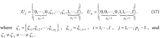
(17)

where

ζ

i=

{

ξ ξ

i,1, i,2,,

ξ

i p, _ξ

}

,

ξ

i j, =

ξ

i j, +1, i=1,,l , j=1,,pξ −1, and

1 2 l

ζ ≠ζ ≠_≠ζ _.

Let m and m′ be the number of knots in the knot vectors U_ξ and U_η, re-spectively. Also, let k and k′ be pξ+1 and pη+1, respectively. Here, if the

function to be approximated has a singularity of type

( )

q r

 with

0< =q nq mq <1, where n mq, q∈, then the polynomial degree of B-spline functions corresponding to U_η is pη =mq.

Let Bi k,

( )

ξ , i=1,,m−k be the B-splines corresponding to the knot

vec-tor U_ξ and let B_{j k,′}

( )

η , j=1,,p_η+1 be the B-splines corresponding to

the knot vector U_η. Here, the B-spline functions Bj k, ′, j=1,,pη +1,

cor-responding to the open knot vector U_η are the Bernstein polynomials of degree p_η.

Consider the control points Pi j, and the weights wi j, for 1≤ ≤ = −i n m k, 1≤ ≤j pη+1, that are listed in Table 1. We now construct a NURBS surface

from the parameter space _Ωˆ _{onto Ω as follows:}

(

)

,

(

)

,

1 1

, , .

n k

i j i j

i j

R

ξ η ′ ξ η = =

=

∑∑

F P

(18) Here Ri j,

(

ξ η,

)

,

1

≤ ≤

i

n

, 1≤ ≤j pη+1, are NURBS basis functions defined

by

(

)

,

( )

₍

,

( )

₎

,

, , ,

, i k j k i j i j

B B w

R

W

ξ η

ξ η

ξ η

′

=

(19) where

( )

,

( )

,

( )

,

1 1

, .

n k

s k t k s t s t

W

ξ η

B

ξ

B

η

w

′

′ = =

=

∑∑

Since Bj k, ′

( )

η is the Bernstein polynomial and Pi j, =

( )

0, 0 unless j=k′,

substituting Equations (13) into (19) the NURBS surface mapping (18) becomes

(

)

,

( )

, ,

(

)

1

, , .

n p

i k i k i k i

p_η η B w W

ξ η η ξ ′ ′ ξ η

=

 

= _{ }



∑



[image:10.595.206.540.66.146.2]

F P

Table 1. Control points Pi j, and weights wi j, .

1≤ ≤j p_η j=p_η+1

i Pi j, wi j, Pi j, wi j,

1 ( )0, 0 β1 (x y1, 1) β1

2 ( )0, 0 β2 (x y2, 2) β2

    

DOI: 10.4236/jamp.2019.77107 1582 Journal of Applied Mathematics and Physics

Now, we derive the derivative of the mapping F

(

ξ η,

)

by using formulas in Chapter 4.5 in [12].

Let

(

)

(

,

₍

) (

₎

,

)

(

₍

,

)

₎

, , , , W W W

ξ η ξ η ξ η ξ η

ξ η ξ η

= F = A

F

where A

(

ξ η,

)

is the numerator of F

(

ξ η,

)

. Denoting ( 1 2)

( )

1 2

( )

1 2 , , , α α α α α α

φ ξ η φ ξ η

ξ η

+

∂ =

∂ ∂ , the derivative of F

(

ξ η,

)

can be expressed as ( )

(

)

(

)

( )

(

) (

)

(

)

( )

1 2 1 2

1 2 , , , , , , , , W W W

α α α α

α α ξ η ξ η ξ η

ξ η ξ η

    =_{ } =_{ }         A F F Then

(

)

( )

₍

_{) (}

₎

( ) ( ) ( ) ( ) ( ) ( ) ( ) ( ) ( ) ( ) ( ) 1 2 1 2 2 1 1 2 1 2 1 2 1

1 2 1 2

2 1 2

1 2 , , ,0 ,0 1 0 , , 1 2 0 0

0,0 , 1 ,0 ,

1

0, ,

2 1

1 1 1

, , ,

i i i

i j i j i j

i i i

j j

j i j

W W i W i j W W i W j i α α α α α α α α α α α α α

α α α α

α α α

α α

ξ η ξ η ξ η α η α α α α α − = − − = = − = − = = = = _ _     ∂ = _{   } ∂         = _{   }       = + _{ }       + _{ } + _{ }    

∑

∑

∑

∑

∑

∑

A F F F F F

F 2 _W( ) (i j, 1 i, 2 j) j

α α

α _{− −}

     

∑

F

(20)

Solving the Equation (20) for F

(

ξ η,

)

, we obtain

(

)

( )

(

)

( ) ( ) ( )

( ) ( )

( ) ( )

1

1 2 1 2 1 2

2

1 2

1 2

1 2

, , 1 ,0 ,

1 0, , 2 1 , , 1 2 1 1 1 , , i i i j j j

i j i j i j W i W W j W i j α

α α α α α α

α α α α α α α α ξ η ξ η α α α − = − = − − = =    = _ − _{ }      − _{ }        − _{    }     

∑

∑

∑

∑

F A F

F

F

(21)

We employ the lemma below from Chapter 3 in [12] in order to determine

( )

(1, 2) , α α

ξ η

A and

( )

( 1, 2) ,

W

ξ η

α α . Lemma 1 Let ( )0

i = i

P P, and

( )

( )0

( )

,

( )

( )0 1

n

i k i i

C

ξ

C

ξ

B

ξ

=

= =

∑

P . Then

( )

_{( )}

1

_{( )}

( )

1 1

1 , 1 n

i k i

i

C B

α

α α

α

ξ − ₋ ξ =

=

∑

P

with ( ) ( ) ( )

(

)

1 1 1 1 1 1 1 1 1 1 , 0 , 0 i i i i i k i

k u u α α α α α

α − − _α

+ + +

= 

 ₋

=  _{− >}

 ₋ 

P P

P P

DOI: 10.4236/jamp.2019.77107 1583 Journal of Applied Mathematics and Physics ( )  1 1 1 1

0, , 0 , _k , , _{m k},1, ,1 .

k k

Uα u u

α α + − − −     =        

Applying the lemma 1 into (21), we have

( )

(

)

( )

( )

1 2

1 2 1

1 , , , 1 2 ! , ! n p

i k i k i

p

B p

η α α

η

α α α

α η

η

ξ

α

− − ′ − =   = _{ } − _

∑

_ A P where ( ) ( ) ( )

(

)

1 1 1 1 , 1 1 1 1 ,

1, , 1

, 0

, 0.

i k i k

i k i k i k i

k u u α α α α α α _α ′ − − ′ ′ ′ + + + =   ₋

=  _{− >}

 ₋ 

P P

P P

The derivative of the total weight function W

(

ξ η,

)

, also, can be described in detail by substituting the Bernstein polynomial into Bj k, ′

( )

η .

(

)

( )

( )

( )

{

₍

₎

}

( )

( )

( )

(

)

(

)

(

)

{

}

( )

(

)

1 2 2 1 1 2 2 ₂ , 1 , , 1 1 , ,1 1 ₂ 1 , , 2 ₂ , 1 1 ! 1 ! ! 1 . 1 ! n k k j j

i k i j

i j

n

p

i k i

i p

k j p

j

i j i k j W p B w j p B w p p p w w j p η η η α α α α η

α η α

η

α _{η α}

η

η

ξ η

ξ η η

ξ η

α

η η η

α ′ ′− − = = − = ′− − − ′ =     = _{  } − _ −       = − −     _ + _{ } − + − −    _

∑

∑

∑

∑

3.3. Numerical Example of Mapping Method for Solving

an Isotropic Elasticity Containing Single Singularity

The mapping method proposed was implemented in the paper [1], and the pa-per showed that the mapping technique using NURBS geometrical mappings constructed by an unconventional choice of control points are effective for nu-merical solutions of elliptic boundary value problems containing a single singu-larity. In this subsection, we solve an elastic problem containing a singularity to show that the proposed method is also applicable to implement elastic problems.

Throughout this paper, we measure the error

(

h

)

u u− of the computed solu-tions obtained by isogeomtric analysis using the proposed mapping method in the following norms:

• _{The relative error in the maximum norm in %:}

( )

,rel % 100

h h u u u u u ∞ ∞ ∞ − − = ×

• _{The relative error in L}2 norm in %:

( )

2

2

2

,rel % 100

h h L L L u u u u u − − = ×

DOI: 10.4236/jamp.2019.77107 1584 Journal of Applied Mathematics and Physics

( )

1

2 2 2

eng eng 2 eng,rel

eng

% 100

h u u

u u

u

 ₋ 

 

− =_{ } ×

 

 

Assuming that the Young’s modulus

E

=

1000

and the Poisson’s ratio

0.3

ν =

in a sector of the unit circle whose the central angle is 270˚, plane strain isotropic elastic body, we consider that the following analytic stress field,

(

)

(

)

(

(

)

)

(

)

(

(

)

)

(

)

(

)

(

(

)

)

(

)

(

(

)

)

(

)

(

(

)

)

(

)

(

(

)

)

1

1

1

2 1 cos 1 1 cos 3 ,

2 1 cos 1 1 cos 3 ,

1 sin 3 1 sin 1 ,

x

y

xy

r q

r q

r q

λ λ λ

σ λ λ λ θ λ λ θ

σ λ λ λ θ λ λ θ

τ λ λ λ θ λ λ θ

− − −

 

= _ − + − − − − _

 

= _ − + − − − − _

 

= _ − − + + − _

(22)

where λ =2 3, and

(

)

(

)

cos 1 0.75π

cos 1 0.75π

q λ

λ −

 

 

=

+

 

 . Then, the stress field (22) satisfies the equilibrium equations of elasticity on the sector shaped domain ΩL. And the displacement field has the singularity of the form 2 3

( )

r

φ θ

where φ θ

( )

is a smooth function.

For the design of the physical domain ΩL, we set pξ =2, pη =3 and

{

}

{

}

1 1 3,1 3 , 2 2 3, 2 3

ζ = ζ = in the knot vector (17) so that the open knot vector corresponding to ξ-direction is as follows:

{

0, 0, 0,1 3,1 3, 2 3, 2 3,1,1,1

}

Uξ =

₍₂₃₎

We construct the open knot vector corresponding to

η

-direction using the form of the knot vector U_η in (17):

{

0, 0, 0, 0,1,1,1,1 ,

}

Uη =

₍₂₄₎

which make Bernstein polynomials in

[ ]

0,1 on the parameter space. We choose

( )

0, 0 for control points P_{i j,} ,i=1,,k

( )

=7 ,j=1,,pη

( )

=3 , and set the other control points as depicted in Figure 4(a). Then the NURBS surface mapping

( )

_{, :}ˆ _, ˆ

[ ] [ ]

_{0,1 0,1 ,}

L L L L

F

ξ η

Ω Ω Ω = ×

and the inverse of the design mapping generates the singularity of the form

( )

1 3

r

φ θ

along the radial direction on the ΩL in Figure 4(a).

In order to enrich the NURBS or B-spline basis functions without failing the structure of the mapping technique, we employ refinements [14], [15] in the NURBS functions which are used to design the physical domain as depicted in Figure 4(a). In particular, we use p-refinement to enrich the basis functions corresponding to both the open knot vectors (24) and (23). Note that inserting new knots to increase the number of basis functions along the

η

-direction may cause malfunction regarding the production of singular functions [11].

Figure 4(b) and Table 2 depict the relative errors of the displacement u and v

in the maximum norm(blue and red line, respectively), and in the L2 norm

[image:13.595.290.456.77.121.2]

DOI: 10.4236/jamp.2019.77107 1585 Journal of Applied Mathematics and Physics

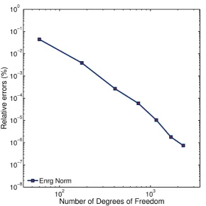
the maximum norm versus the number of degrees of freedom. Both Figure 4(b) and Figure 4(c) show that the proposed mapping method captures the singular-ity effectively, and follows the theoretical results in [1]. Figure 5 exhibits the rel-ative errors of the strain energy of the stress field.

[image:14.595.62.543.205.645.2]

4. Patchwise NURBS Mapping Method for Solving Elliptic

Boundary Value Problems Containing Multiple Singularities

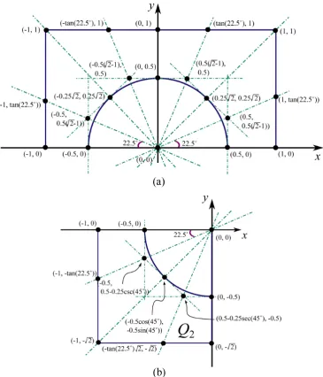
In the case of that a physical domain contains multiple cracks, we re-design the

Figure 4. (a) The NURBS surface F_L

(

ξ η,

)

maps from the parameter space Ω =ˆL

[ ] [ ]

0,1× 0,1 to the sector shaped domain ΩL.

The coordinates of the primary control points Pi p,η+1,i=1,,7 are described. (b) Relative errors of the displacement field

{ }

u

in the maximum norm and L2 norm for (22) (c) Relative errors of the stress field

{ }

σ in the maximum norm for (22). (a) The

scheme of the NURBS surface FL that generates singular functions; (b) Relative errors of the displacement field { }u ; (c) Relative

[image:15.595.208.538.101.370.2]

DOI: 10.4236/jamp.2019.77107 1586 Journal of Applied Mathematics and Physics

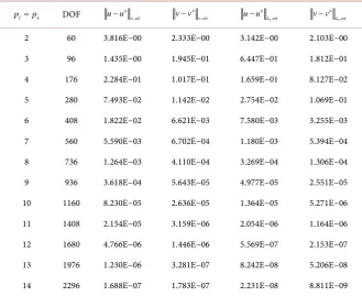
Table 2. The relative errors (%) of the elasticity containing singularity on the sector shaped elastic material (22): relative errors (%) of displacement field.

p_ξ=p_η DOF

,rel h

u−u _∞

,rel h

v−v _∞

2,rel h

L

u−u

2,rel h

L

v−v

2 60 3.816E−00 2.333E−00 3.142E−00 2.103E−00

3 96 1.435E−00 1.945E−01 6.447E−01 1.812E−01

4 176 2.284E−01 1.017E−01 1.659E−01 8.127E−02

5 280 7.493E−02 1.142E−02 2.754E−02 1.069E−01

6 408 1.822E−02 6.621E−03 7.580E−03 3.255E−03

7 560 5.590E−03 6.702E−04 1.180E−03 5.394E−04

8 736 1.264E−03 4.110E−04 3.269E−04 1.306E−04

9 936 3.618E−04 5.643E−05 4.977E−05 2.551E−05

10 1160 8.230E−05 2.636E−05 1.364E−05 5.271E−06

11 1408 2.154E−05 3.159E−06 2.054E−06 1.164E−06

12 1680 4.766E−06 1.446E−06 5.569E−07 2.153E−07

13 1976 1.230E−06 3.281E−07 8.242E−08 5.206E−08

14 2296 1.688E−07 1.783E−07 2.231E−08 8.811E−09

Table 3. The relative errors (%) of the elasticity containing singularity on the sector shaped elastic material (22): The computed strain energy and the relative errors (%) of the stress field

{ }

σ . The row “∞_{” indicates the exact values.}

p_ξ=p_η DOF h _,rel

x x σ −σ _∞

,rel h y y σ −σ _∞

,rel h xy xy

τ −τ _{∞ Strain Energy}

2 60 6.334E+03 9.922E+03 1.483E+04 88.98117013046564

3 96 3.670E+02 1.818E+02 2.030E+02 89.14930415746228

4 176 2.556E+02 3.853E+02 9.833E+02 89.15648698854705

5 280 6.185E+01 5.250E+01 1.091E+02 89.15771576771605

6 408 2.072E+01 3.242E+01 8.419E+01 89.15782485559064

7 560 5.732E−00 3.710E−00 6.687E−00 89.15782012258868

8 736 1.457E−00 2.070E−00 5.457E−00 89.15781818638276

9 936 5.276E−01 3.246E−01 5.544E−01 89.15781843245076

10 1160 1.049E−01 1.372E−01 3.657E−01 89.15781850351074

11 1408 3.942E−02 2.152E−02 3.261E−02 89.15781849595437

12 1680 6.713E−03 7.708E−03 2.116E−02 89.15781849355913

13 1976 2.915E−03 1.782E−03 2.515E−03 89.15781849380155

14 2296 6.877E−04 9.680E−04 2.107E−03 89.15781849389655

[image:15.595.190.535.427.737.2]

[image:16.595.231.522.65.355.2]

DOI: 10.4236/jamp.2019.77107 1587 Journal of Applied Mathematics and Physics

Figure 5. Relative errors of the strain energy of the stress field (22) on the sector shaped elastic body.

geometrical mapping by using both standard NURBS mappings and the pro-posed mappings. Then it simplifies things to describe these sub-domains by dif-ferent patches. We describe how to construct the set of global basis functions crossing interfaces between patches. Throughout the following examples, we show that the patchwise mapping method is effective in dealing with a problem containing multiple singularities.

First, We apply the mapping method for the elliptic boundary value problems with multiple singularities of type

( )

i i

rλ

ψ θ

, where 0< <l 1, and ψi’s are smooth functions. Example 1. Let

(

)

(

)

1 2 1 2

1 1 cos 1 2 2 sin 2 2 , 1, and 1

u =r

θ

+r

θ

f = −∆u g =u _Γ where

[

]

(

)

(

)

1

2 2

2 2

1 2

1 1

1 2

1 2

1,1 0,1 2

, 1 1 2

1

cos , cos

r x y r x y

x x

r r

θ − θ −

 

Ω = − ×_ + _

= + = − + − −

   − 

= _{ } = − _{ }

   

(25)

Then u1 is the analytic solution of the Poisson equation:

1 1

in and on

u f u g

DOI: 10.4236/jamp.2019.77107 1588 Journal of Applied Mathematics and Physics

and has two singularities at

( )

0, 0 and

(

1,1+ 2

)

.

4.1. Patchwise NURBS Mappings and Interfaces

In Example 1, we divide the physical domain into three patches:

[

] [ ]

[ ]

[

]

1,1

1,2

1,3

1,1 0,1 0,1 1,1 2

1, 0 1,1 2

Ω = − ×

 

Ω = ×_ + _

 

Ω = − ×_ + _

Let Ω1,i’s are physical patches. We construct NURBS geometrical mappings

1,1

F and F1,2 that generate singularities of the type

( )

1 2

1 1

r

ψ θ

and 1 2

( )

2 2

r

φ θ

, respectively. They are also the design maps from the parameter space Ωˆ1,i to the physical patch Ω1,i, for each i=1, 2. To build up F1,i,i=1, 2 we use the following knot vectors: For F1,1,

{

}

{

}

1 2 3 0, 0, 0, , , ,1,1,1

0, 0, 0, 0.5, 0.5,1,1,1 , U

U

ξ η

ζ ζ ζ =

=

(27)

where ζ1=

{

0.25, 0.25

}

, ζ2 =

{

0.5, 0.5

}

, and ζ3=

{

0.75, 0.75

}

. For F1,2,

{

}

{

}

1 0, 0, 0, ,1,1,1

0, 0, 0, 0.5, 0.5,1,1,1 , U

U

ξ η

ζ =

=

where ζ1=

{

0.5, 0.5

}

.

In the design mappings, we observe the following:

1) We employ control points and weights from Example 5.3 in [1] to build

1,1

F , and primary control points are shown in Figure 6(a).

2) We design the NURBS geometrical mapping Fˆ1,2

( )

ξ η

, that generates a

singularity

(

)

(

)

1 4

2 2 1

1 2

2 2

cos x

x y

x y

ψ −

  

  

+ _{  }

 

 _ + _

 

using the control points as

de-picted in Figure 6(b).

3) Using the affine transformation we define

(

)

(

(

)

)

1,2 , ˆ1,2 1, 1 2 .

F ξ η ≡F ξ+ η+ +

In Figure 6, the quasi-physical patch is a physical patch translated.

4) Since a singularity does not appear in the patch Ω1,3, we employ the

stan-dard NURBS design technique to build the mapping F1,3

(

ξ η,

)

from the

para-meter space Ωˆ1,3 to Ω1,3.

4.2. Construction of Global Basis Functions over Interfaces and

Approximation Space

Now, we construct an approximation space by using B-spline functions which were used in the design mapping F1,i. First, we consider connectivity among

B-spline functions defined on different patches and are nonzero along the inter-face as depicted in Figure 7(a). To obtain 0

[image:18.595.172.538.68.495.2]

DOI: 10.4236/jamp.2019.77107 1589 Journal of Applied Mathematics and Physics

Figure 6. Primary control points of the NURBS geometrical mapping F1,1

( )

ξ η, and Fˆ1,2

(

ξ η,

)

from Ωˆ1,i to (a) the physical patch Ω1,1 (b) the quasi-physical patch Q2 which has the

singu-larity at the origin. F1,2

( )

ξ η, is constructed by composition of Fˆ1,2 with an affine transformation,

and Fˆ1,2 maps from the parameter space, Ωˆ1,2 to the physical space Ω1,2. (a) Primary control

points and design of the physical patch Ω1,1; (b) Primary control points and design of the

qua-si-physical patch Q2.

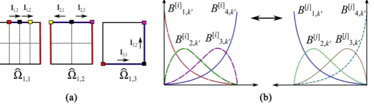
an interface between two different patches, we merge two B-spline local basis functions defined on different patches that have the same nonzero value on the interface between the two patches. In Figure 8(a), Ii j, ’s represent intervals

cor-responding to the interface on the physical domain in Figure 7(a). In Ii j, , the

index i means the index of the patch belonging to the interval, the other index j

indicate the index of patch such that

( )

(

)

1

[image:19.595.170.539.61.254.2]

DOI: 10.4236/jamp.2019.77107 1590 Journal of Applied Mathematics and Physics

Figure 7. The control points for NURBS surface with (a) three patches for the Example 1, and (b) three patches for the Example 2, respectively. (a) The control points with two singularities; (b) The control points with two singularities.

Figure 8. (a) Ij l, represents the interval along ξ- or η-directions corresponding to the interface in

the physical domain. We follow directions of arrows when we set the global index. (b) We merge two B-spline basis functions which are interpolants for each parameter space. (a) Parameter spaces of F1,i’s; (b) Construction of new basis function from two interpolant B-spline basis functions

de-fined on two distinct parameter space.

To construct global basis functions which are nonzero functions on

, ,,

i j j i

I I i≠ j, we merge the nonzero basis function in Ii j, and the nonzero

basis function in Ij i, , where i≠ j such that they are reflection about the interface

( )

( )

1,i i j, 1,j j i,

F I =F I in the physical domain. In Figure 8(b), for example, let [ ]

_{( )}

, i s k

B ′

η

and [ ],

( )

, 1, 2, 3, 4 j

s k

B ′

η

s= be B-spline basis functions of

η

in Ω1,1

and Ω1,3, in Figure 8(b), respectively. Note that i and j in the bracket

[ ]

⋅

represent indices of patches. So

i

=

1

and j=3. Let Bt k[ ]1,

( )

ξ

and

[ ]3

_{( )}

, t k

B

ξ

be

B-spline basis functions of ξ such that

[ ]

₍

₎

1,3 1

, 0 when 1, , 2 1 1

t k I

B t p_ξ p_ξ

ξ∈ ≠ = +  + −

[ ]

3,1 3

, 0 when 1, , 1.

t k I

B t p_ξ

ξ∈ ≠ =  +

Because

• [ ]

( )

[ ]

( )

1,3 3,1

1 3

4,k 1,k 1

I I

[image:19.595.172.543.307.411.2]

DOI: 10.4236/jamp.2019.77107 1591 Journal of Applied Mathematics and Physics

•

(

[ ] [ ]

)

(

)

_{( )}

(

[ ] [ ]

)

(

)

_{( )}

1 _{1,1 1,3} 2 _{1,3 3,1}

1 1 1 3 3 1

4, 1,1 1, 1,1

, k , , k ,

t k _{F I} t k _{F I}

B ⋅B ′ F− x y = B ⋅B ′ F− x y ,

•

(

t t1,2

)

=

(

pξ +1,1 ,

) (

pξ +2, 2 ,

)

, 2

(

(

pξ + −1

)

1,pξ +1

)

,

•

(

[ ] [ ]

)

(

[ ] [ ]

)

1 2

1 1 3 3

4, 1,

, k , k

t k t k

B ⋅B ′ = B ⋅B ′ on the inter face F1,1

( )

I1,3

(

=F1,3

( )

I3,1

)

.

We merge two B-spline basis functions

(

[ ]1 [ ]

)

1 1

4,

, k

t k

B ⋅B ′ and

(

Bt k[ ]₂3, ⋅B1,[ ]3k′

)

so that we count the new function as one global basis function. The new function has a nonzero value on two distinct patches. Here, we should carefully set

(

t t1, 2

)

,

and we apply the same degree of p-refinement into each parameter space. For a space with the non-homogeneous boundary condition in Example 1,

(

)

( )

{

1

}

1 2

1= w x y, ∈H Ω1 :w∂Ω =g,Ω ⊂1 



(28) We decompose the space (28) into

(

)

( )

{

1

}

1 2

1,1= w x y, ∈H Ω1 :w∂Ω = Ω ⊂0, 1 



and

(

)

( )

{

1

}

1 2

1,2= w x y, ∈H Ω1 :w∂Ω =g,Ω ⊂1 .

 

The finite dimensional subspace i.e. approximation space of the Poisson equa-tion (26) is

{

}

1 1,1 1,2 1 2: 1 1,1, 2 1,2 ,

h h h h h

w w w w

= ⊕ = + ∈ ∈

    

1,1 1,1, 1,2 1,2, h_⊂ h _⊂

   

1, span ,1 ,1 ,2 ,2 ,3 , 1, 2

h new new

i=  i  i  i  i  i  i=

     

[ ] [ ]

(

)

{

1 1 1

}

1,1 Bi k, Bj k, F1,1 :i 2, ,n1 1, j 2, ,n1 1 , − ′ ′ = ⋅ _ = _ − = _ −  [ ] [ ]

(

)

{

2 2 1

}

1,2 Bi k, Bj k, F1,2:i 2, ,n2 1, j 2, ,n2 1 , − ′ ′ = ⋅ _ = _ − = _ −  [ ] [ ]

(

)

{

3 3 1

}

1,3 Bi k, Bj k, F1,3:i 2, ,n3 1, j 2, ,n3 1 , − ′ ′ = ⋅ _ = _ − = _ −  [ ] [ ]

(

)

{

(

)

}

1 1 1

2,1 , , 1,1 1 1

1 1 1

: 1, , when 1,

and 1, , , 1 , , when ,

i k j k

B B F j n i n

i p n_ξ p_ξ n j n

− ′ ′ = ⋅ = = ′ = − − =      (29) [ ] [ ]

(

)

{

2 2 1

}

2,2 Bi k, Bj k, F1,2: j 1, ,n2 1 wheni 1,n2 , − ′ ′ = ⋅  =  − =  [ ] [ ]

(

)

{

}

3 3 1

2,3 , , 1,3 3

3 3

: 2, , when 1

and 2, , 1 when ,

i k j k

B B F j n i

i n j n

− ′ ′ = ⋅ = = ′ = − =     [ ] [ ]

(

)

(

)

{

1 , 1 , 1

}

1,1 , , 1,1 : 2, , 1 1 , 1 ,

new new

new

i k j k

B B ′ F− i pξ n pξ j n′

= ⋅ _ = + _ − + =



[ ] [ ]

(

)

{

2 , 2 , 1

}

1,2 , , 1,2 : 2, , 2 1, 1, 2 ,

new new

new

i k j k

B B ′ F− i pξ n i pξ j n′

= ⋅ _ = + _ − ≠ + =



[ ] [ ]

(

)

{

1 , 1 , 1

}

2,1 , , 1,1 : 1, 1 , 1 ,

new new

new

i k j k

B B ′ F− i pξ n pξ j n′

= ⋅ _ = + − =

DOI: 10.4236/jamp.2019.77107 1592 Journal of Applied Mathematics and Physics

[ ] [ ]

(

)

{

2 2

}

2 , 2 , 1

2,2 , , 1,2 ,

new new

new

n k n k

B B′ ′ F−

= ⋅ _



where

1) ni and ni′ are the number of B-spline functions in ξ- and η-direction of the patch Ω1,i, respectively.

2) [ ], [ ], , , , i new j new s k t k

B B ′ are new global basis functions by merging two B-spline

functions in Ω1,i and Ω1,j, respectively of ξ and

η

, respectively. 3) 1,i and 1,

new i

 are the set of B-spline basis functions composition with the inverse of NURBS surface mapping F1,i on the physical domain Ω1

satis-fying homogeneous boundary condition. 4) 2,i and 2,

new i

 are the set of B-spline basis functions composition with the inverse of NURBS surface mapping F1,i on the physical domain Ω1

[image:21.595.55.543.96.679.2] [image:21.595.65.536.392.685.2]

satis-fying non-homogeneous boundary condition.

Figure 9 shows the relative errors (%) versus DOFs. In Figure 9(a) and Table 4, we enrich the set of basis functions by p-refinement and increase the degree of polynomial pξ and pη up to 14. The DOF is 3061 when pξ = pη =15. We

can see that the proposed mapping method is effective to capture multiple sin-gularities as well as a single crack or singularity.

Example 2. Let 2 3 2, 1

i i=

Ω = Ω

_

_{be the unit disk, where} Ω_2,i’s are minor sec-tors whose central angles are 120˚ for each i=1, 2,3, and

( )

3 1 2

(

)

2 2 2

1

, _i cos _i 2 , and

i

u x y r

θ

f u g u _Γ

=

=

∑

= −∆ =

Figure 9. The relative error (%) in the maximum norm, the L2_{-norm, and the energy norm of the computed solutions of the}

[image:22.595.204.538.114.407.2]

DOI: 10.4236/jamp.2019.77107 1593 Journal of Applied Mathematics and Physics

Table 4. The relative errors (%) of the Poisson equation on the rectangle (26): The com-puted strain energy and the relative errors (%) of the approximate solution h

u . The row

“∞_{” indicates the exact values.}

p_ξ=p_η DOF h _,rel

u−u _∞

2,rel h

L

u−u

eng,rel h

u−u Strain Energy

2 71 5.376E−01 4.968E−01 1.219E−00 1.9224816355887329

3 145 1.358E−01 4.062E−02 1.014E−00 1.9223933783586342

4 245 2.655E−02 1.083E−02 3.504E−01 1.9221720544391365

5 371 6.469E−03 3.201E−03 1.482E−01 1.9221998800087665

6 523 1.613E−03 4.345E−04 6.126E−02 1.9221949350016059

7 701 4.077E−04 6.766E−05 2.950E−02 1.9221958237730838

8 905 1.031E−04 2.624E−05 1.424E−02 1.9221956174946071

9 1135 2.433E−05 6.642E−06 6.643E−03 1.9221956649732888

10 1391 5.681E−06 1.028E−06 3.238E−03 1.9221956544748704

11 1673 1.302E−06 2.510E−07 1.508E−03 1.9221956569276313

12 1981 2.926E−07 9.886E−08 8.398E−04 1.9221956563547675

13 2315 6.736E−08 2.099E−08 1.512E−04 1.9221956564947542

14 2675 2.232E−08 4.300E−09 4.330E−04 1.9221956564543110

∞ 1.9221956564903575

where

2 2

, ,

i

ix i

i ix iy

iy i

t x x

r t t T

t α y y

 + 

   

 

= +  =  ₊ 

   

   

( )

( )

( )

( )

cos sin

, 1, 2, 3

sin cos

i

i i

i i

x x

T i

y y

α

α α

α α

 − 

 ₌   ₌     

   

   

(30)

1 0.68 cos12 , 1 0.68sin12 , 1 12

x = −  y = −  α = 

2 0.7 cos150 , 2 0.7 sin150 , 2 150

x = −  y = −  α = 

3 0, 3 0.5sin 90 , 3 90

x = y =  α = 

1

1

cos if 0,

cos if 0

i

i i

i

i

x x

y r

x x

y r

θ

−

−

  + 

>

  

  

= 

 + 

−   ≤

 _{ }



Then u2 solves the following elliptic boundary value problem:

2 2

in and on ,

u f u g

−∆ = Ω = Γ = ∂Ω

₍₃₁₎

and the solution u2 has three crack singularities at

(

x yi, i

)

,i=1, 2, 3.

DOI: 10.4236/jamp.2019.77107 1594 Journal of Applied Mathematics and Physics

(

)

{

}

(

)

{

}

(

)

{

}

2,1 1 1 1 1

2,2 1 1 1 1

2,3 1 1 1 1

, | 0 1, 150 270

, | 0 1, 270 390

, | 0 1, 30 150

r r

r r

r r

θ

θ

θ

θ

θ

θ

Ω = ≤ ≤ ≤ ≤



Ω = ≤ ≤ ≤ ≤

 

Ω = ≤ ≤ ≤ ≤



 

 

 

Then, we build a design mapping Fˆ2,i

( )

ξ η

, from the parameter space Ωˆ2,i to a quasi-physical sector Qi using the proposed mapping method, for

1, 2,3

i= . Here, we define three physical patches Ω2,i by using quasi-physical sectors Qi as follows:

(

) ( )

{

}

2,i x x yi, yi | x y, Qi ,

Ω = + + ∈

which means that Qi’s are sectors having the same radii and the central angles as these of Ω2,i’s through the transformation (30) but the position of the crack tip in Qi is the origin other than

(

x yi, i

)

in Ω2,i for i=1, 2,3. A structural drawing detailed for Q1 and Q2 is shown in Figure 10, and Q3 is designed

by rotating Q1 to −90˚. Finally, we define the NURBS geometrical mapping

that generates singularities as follows:

( )

( ) (

)

2,i , ˆ2,i , i, i . F

ξ η

≡F

ξ η

+ x y

[image:23.595.61.540.387.639.2]

Similar to that of Example 1, considering the continuity of the basis functions and the construction of the basis functions on interfaces, we merge two basis

Figure 10. The NURBS geometrical mapping Fˆ2,i

(

ξ η,

)

from Ωˆ2,i to the quasi-physical patch Qi whose crack tip is the origin,

generates the singularity of the type 1 2

( )

i i

r ψ θ , for i=1, 2,3. Once we design the mappings, we update them by composition with

transformation so that the final NURBS geometrical mapping preserving the mapping technique in Fˆ2,i maps from the

parame-ter space, Ωˆ2,i to the physical sector Ωi, for i=1, 2,3. (a) Primary control points and design of the quasi-physical patch Q1; (b)