Data Mining of Spatio Temporal Variability of Chlorophyll a Concentrations in a Portion of the Western Atlantic with Low Performance Hardware

ISSN Online: 1945-3124 ISSN Print: 1945-3116

DOI: 10.4236/jsea.2019.125010 May 31, 2019 149 Journal of Software Engineering and Applications

Data Mining of Spatio-Temporal Variability of

Chlorophyll-a Concentrations in a Portion of

the Western Atlantic with Low Performance

Hardware

Italo F. Di Paolo

_{, Nelson A. Gouveia}

_{, Luiz C. Ferreira Neto}

_{, Eduardo T. Paes}

_,

Nandamudi L. Vijaykumar

_{, Ádamo L. Santana}

1_{Center for Natural Sciences and Technology (CCNT), Pará State University (UEPA), Belém, Brazil} 2_{National Institute for Space Research (INPE), São José dos Campos, Brazil}

3_{Institute of Technology (ITEC), Federal University of Pará (UFPA), Belém, Brazil}

4_{Socio-Environmental Institute and Water Resources (ISARH), Federal Rural University of Amazonia (UFRA), Belém, Brazil}

Abstract

The contemporary scientific literature that deals with the dynamics of marine chlorophyll-a concentration is already customarily employing data mining techniques in small geographic areas or regional samples. However, there is little focus on the issue of missing data related to chlorophyll-a concentration estimated by remote sensors. Intending to provide greater scope to the identi-fication of the spatiotemporal distribution patterns of marine chlorophyll-a concentrations, and to improve the reliability of results, this study presents a data mining approach to cluster similar chlorophyll-a concentration beha-viors while implementing an iterative spatiotemporal interpolation technique for missing data inference. Although some dynamic behaviors of said con-centrations in specific areas are already known by specialists, systematic stu-dies in large geographical areas are still scarce due to the computational com-plexity involved. For this reason, this study analyzed 18 years of NASA satel-lite observations in one portion of the Western Atlantic Ocean, totaling more than 60 million records. Additionally, performance tests were carried out in low-cost computer systems to check the accessibility of the proposal imple-mented for use in computational structures of different sizes. The approach was able to identify patterns with high spatial resolution, accuracy and relia-bility, rendered in low-cost computers even with large volumes of data, gene-rating new and consistent patterns of spatiotemporal variability. Thus, it How to cite this paper: Di Paolo, I.F.,

Gouveia, N.A., Neto, L.C.F., Paes, E.T., Vijaykumar, N.L. and Santana, Á.L. (2019) Data Mining of Spatio-Temporal Variabili-ty of Chlorophyll-a Concentrations in a Portion of the Western Atlantic with Low Performance Hardware. Journal of Soft-ware Engineering and Applications, 12, 149-170.

https://doi.org/10.4236/jsea.2019.125010

Received: April 16, 2019 Accepted: May 28, 2019 Published: May 31, 2019

Copyright © 2019 by author(s) and Scientific Research Publishing Inc. This work is licensed under the Creative Commons Attribution International License (CC BY 4.0).

DOI: 10.4236/jsea.2019.125010 150 Journal of Software Engineering and Applications opens up new possibilities for data mining research on a global scale in this field of application.

Keywords

Data Mining, Clustering, Chlorophyll, Atlantic, Missing Data, Small Hardware

1. Introduction

At a global level, phytoplankton organisms are responsible for net primary pro-duction of 50 petagrams of carbon per year [1] and chlorophyll-a concentrations in the ocean, commonly used as a proxy of phytoplankton biomass, become an important variable in the ecological study of marine and coastal environments.

When interacting with electromagnetic radiation in the visible range (400 - 700 nm), phytoplankton absorbs more energy at the wavelength of the blue re-gion (400 - 500 nm) and reflects more in the green rere-gion (500 - 600 nm) [2]. This relationship between absorbed and reflected energy in the blue and green bands provides the basis for quantifying the concentrations of said energy in the oceans by means of Remote Sensing at the orbital level.

The works of [3] [4] [5] showed the importance of chlorophyll-a concentra-tions by remote sensing in the demarcation of marine ecoregions. These regions provide an understanding of the interaction and control mechanisms of physi-cal, chemical and biological processes that reflect the diversity of the ocean en-vironment.

On clustering in regions, in data mining-related studies, the work of [3] used a 1˚ × 1˚ spatial resolution, which is equivalent to a distance of approximately 110 km between each point. The works of [5] [6] have also applied a clustering using a 1˚ × 1˚ resolution. Currently, due to orbital satellite sensors, finer spatial reso-lution products are available, of approximately 4 km or 9 km; this allows for more accurate discrimination of oceanic regions that have seasonal and tempor-al variability characteristics of chlorophyll-a.

These modern sensors are fairly applied in the study of ocean color. The physical principle involved in the process of obtaining biological variable takes place by capturing the energy reflected by the Earth’s surface through optical sensors and converting each measurement into a digital number represented by a pixel. This numerical record of a pixel goes through atmospheric and radi-ometric corrections, which are then transformed into chlorophyll-a concentra-tions by using empirical algorithms, described initially by [7]. This procedure was created by adjusting a function from the relationship between the blue and green bands with in situ data, thus enabling studies on a global scale.

DOI: 10.4236/jsea.2019.125010 151 Journal of Software Engineering and Applications the image. Some ocean areas are mostly cloudy and rarely have any ocean color data [7], and this greatly impairs several spatiotemporal analyses.

Regarding the identification of chlorophyll-a concentration variability pat-terns through data mining in large geographical areas and for long periods of time, two major problems were effectively addressed: missing data inference and data mining. Missing data are caused mainly by clouds and data mining is fo-cused on the clustering task. In both cases, processing was fofo-cused on low-cost computers, thus allowing for greater dissemination of these studies, not limited to research centers with large hardware structure available or additional ex-penses contracting cloud computing services.

With respect to the treatment of missing data, many data mining papers that assess the spatiotemporal dynamics of marine chlorophyll concentrations simply ignore them, using for analysis only the effectively observed data [8]-[17]. In re-gions near the equator, such as the sea near the Amazon coast, for example, the amount of missing data is very high and ignoring them can lead to analysis errors; and, for this reason, efficient missing data processing mechanisms are important.

Due to hardware restrictions for data mining in large geographical areas and long historical periods, typically small areas are processed in more accessible computer systems, such as PCs and Notebooks [9] [13]-[18]. Therefore, con-ducting studies related to clusterings or other mining techniques with these data on a global scale is still a challenge, especially on low-cost computers. In turn, the use of parallel or distributed programming, or yet large computer systems increase the cost of the investment in this type of study.

The objectives of the work described herein are: 1) to quantify in time and space the data not recorded (missing data) by the orbital sensors in the Western Atlantic Ocean; 2) to develop and evaluate the efficiency of an algorithm capable of solving the problem of missing data; 3) to cluster regions based on the spati-otemporal variability of chlorophyll-a concentrations; and 4) to implement all the analyses with reduced computational complexity, allowing for processing them in low-cost computers.

This paper is organized as follows: Section 2 presents the materials and me-thods used and defines the study area, acquisition of data, estimation of missing data, and database normalization, thus describing details of the hardware and software settings for processing in common computer systems. Section 3 presents the experimental results obtained, describing the assessment of the missing data inference, the result of chlorophyll-a concentration clusterings in a portion of the Western Atlantic. The discussion of the results is presented in Section 4, highlighting the computational analysis and innovation points in this study, and a qualitative assessment of the patterns that were identified. Finally, Section 5 presents the conclusions.

2. Materials and Methods

DOI: 10.4236/jsea.2019.125010 152 Journal of Software Engineering and Applications source of the survey data and the procedures for obtaining and selecting the data of interest for processing. Also, the procedures for estimating the missing data, data normalization, and software and hardware settings used in the experiments are presented.

2.1. Area of Study

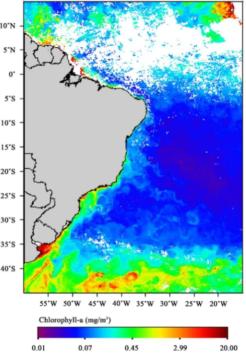
The area of study comprises a portion of the Atlantic Ocean between 45˚S and 15˚N, and 15˚W and 60˚W for latitude and longitude, respectively, as shown in Figure 1. This region has important ecoregions, as seen in [3] [5]; it is also cha-racterized by major problems regarding missing values, especially in the area of the Intertropical Convergence Zone above the equator.

2.2. Acquisition and Selection of Chlorophyll-a Data

Monthly records were obtained for chlorophyll-a with 9 km of spatial resolution from the Giovanni platform [19] of the SeaWiFS/SeaStar sensor between Sep-tember/1997 and December/2007, and the Modis/Aqua, from January/2008

DOI: 10.4236/jsea.2019.125010 153 Journal of Software Engineering and Applications through May/2015. Equation (1) shows the procedure to calculate the

concen-tration of chlorophyll-a, in that logmax

(

(

_{( )}

)

)

Rs X

Rs

= _{for the}

SeaWifs and logmax

(

₍

(

₎

)

)

Rs

= _{for the MODIS, and Rs is the value}

of the surface reflectance in the wavelength indicated.

[

]

(

)

0 1 2 3 4

10a a X a X a X a X

Chlorophyll = + + + + ₍₁₎

The coefficients a a a a a0, , , ,1 2 3 4 of the polynomial, for each sensor, can be

obtained in [20]. These data were concatenated for obtaining a longer time se-ries, totaling 213 images for the period between September/1997 and May/2015.

2.3. Data Analysis

2.3.1. Assessment of Missing Data

The raw data extracted directly from the Giovanni Platform have the following characteristics:

 83,082,993 pixels, or points of observation in the space-time dimensions.

 Missing data: 27,972,128 pixels (33.67% of the total).

It is important to note that the pixels of the continental region, which are not of interest in this research, are included in these raw data. In addition, there are points in the marine region in which the majority of the data in time is also missing, i.e., such data could not be estimated by the satellites, and this inhe-rently precludes reliable inference. So, it was decided that latitude-longitude pairs with over 80 months without estimates are eliminated, as these are consi-dered impractical for measuring a reliable value.

After this analysis and counting out the pixels located on the continental coordinates, 10,814,931 pixels, or 13.02% of the total data, were removed, while still remaining a high total amount of 62,317,197 pixels to process. After com-pleting this initial data selection process, the following distribution was obtained for the following steps:

 7,207,558 pixels, or 11.57%, with negative values of chlorophyll-a concentra-tion, characterizing the missing data that should be estimated.

 55,109,639 pixels, or 88.43%, with values greater than or equal to 0 of chlo-rophyll concentration (mg/m³, with an accuracy of 3 decimal places).

2.3.2. Estimation of Missing Data and Data Normalization

The step to estimate the missing data is antecedent to the cluster processing and is crucial, as the simple deletion of said data from processing can lead to distor-tions in the visualization of processed results.

DOI: 10.4236/jsea.2019.125010 154 Journal of Software Engineering and Applications Algorithm 1. Iterative spatiotemporal interpolation algorithm.

Step 1 maintains all the pixels with valid concentration estimates: greater than or equal to zero. Step 2 defines that, as long as there are data to be processed, one must first calculate the temporal average of the pixel based on the values of the previous and subsequent month. Then, for those that were left or have not been measured, the neighborhood average is calculated with at least 5 neighboring pixels.

These two temporal (previous and subsequent month) and spatial (neighbor-ing pixels) parameters can be modified to achieve greater or lesser precision. Steps 2.a and 2.b are repeated until there are no more pixels to be treated.

The goal of this approach is to favor the temporal average between the pixels, since the chlorophyll-a concentration variation occurs in a non-linear way. Thus, the simple average between the neighbors of the border at the same time moment might not represent the closest value, while using this possibility as a second alternative and by repeating steps 2.a and 2.b until there are no more missing data.

To evaluate the results obtained for the estimation of missing data, the fol-lowing indicators were used: 1) Skill (Equation (2)), which measures the effec-tiveness of the computational model used to infer the missing data [21]; 2) Pearson coefficient of determination r2 _{(Equation (3)); 3) and a graphical}

analy-sis of dispersion, conducted in a partitioned form for better qualitative assess-ment due to the large volume of data.

(

)

2

2

1 Model Obs

Model Obs Obs Obs

X X

Skill

X X X X

− = −

− + −

∑

∑

(

)

(

)

Obs Model Obs

Obs Model

Obs Model

X

X X X

n r X X X X n n  ₋      =      ₋   ₋       ⋅   

∑

∑

∑

∑

∑

∑

∑

where XObs represents the actual values and XModel represents the values

es-timated by the interpolation algorithm.

algo-DOI: 10.4236/jsea.2019.125010 155 Journal of Software Engineering and Applications rithm. Therefore, a methodology for removing known pixels and application of the estimating algorithm had to be developed. In this sense, some of the original data of the Giovanni Platform were taken out at random, and the iterative spati-otemporal interpolation algorithm was used to infer them. Four scenarios were drawn up following this proposal: by removing 5%, 10%, 15% and 20% of the es-timated data.

2.3.3. Clustering

For cluster analysis, it was necessary to normalize the data of the chlorophyll-a concentration for each pixel. Normalizing is necessity for this application, since in certain regions in the area of study, such as the center-south region, variations are very small, thus rendering the analysis of patterns biased, since this analysis interprets those small values as a large cluster of similar behavior.

In this sense, two normalization approaches were used. One of them refers to the calculation of the natural log of the value of each pixel. In the logarithmic scale, very small numerical variations in the mg/m3 _{unit generate increased}

nu-merical variations, thus providing for greater nunu-merical distinction amongst variations and facilitating cluster analysis. This logarithmic scale approach is al-so discussed in the work of [11] [13] [14]. In another approach, the monthly av-erages and standardized anomalies (Equation (4)) were calculated.

Anomaly C Cn

σ −

= ₍₄₎

where C represents the pixel value, C the average for the month corresponding to the pixel C and σ represents the standard deviation for the pixel-related month of C.

To perform spatiotemporal classification of chlorophyll-a concentrations, the clustering with k-means algorithm was used, following the work of [22] [23] [24] was used. The works of [4] [10] [17] [23] [25], also applied this algorithm with similar applications on marine systems, including chlorophyll concentrations.

Since the analysis of the k-means requires previous knowledge of the number of existing clusters in the data being analyzed, a computational methodology was developed for determining these clusters. This consists of several tests with dif-ferent numbers of clusters. For each of them, the dynamics and the distance from each cluster with one another is calculated. The impact of the number of “k” clusters is that where the clusters have greater distinctions amongst them-selves, which is graphically observed with larger or smaller resolutions of the spatiotemporal dynamics. That is, the higher the value of k, the higher the reso-lution of the spatiotemporal dynamics presented in images.

2.3.4. Settings for Processing in Low-Cost Computers

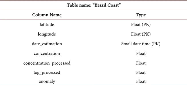
DOI: 10.4236/jsea.2019.125010 156 Journal of Software Engineering and Applications Table 1. Structure of the Brazil coast table.

Table name: “Brazil Coast”

Column Name Type

latitude Float (PK)

longitude Float (PK)

date_estimation Small date time (PK)

concentration Float

concentration_processed Float

log_processed Float

anomaly Float

columns are the numerical coordinates for the spatial location of the pixel, and along with the field “date_estimation”, corresponding to the date of the estimate (month and year, the day was irrelevant), make up the Primary Key (PK) of the table. The “concentration” field corresponds to the value of the chlorophyll con-centration obtained in the Giovanni Platform and the “concentra-tion_processed” field shows the value after the missing data estimation step. It should be noted that the negative values of chlorophyll concentration obtained in the Giovanni Platform are missing data and start having a value greater than or equal to zero after data inference. The “log_processed” field contains the nat-ural log field value “concentration_processed”, and the “anomaly” field has the result of Equation (4) to the value of the “concentration_processed” field.

The function feature of MySQL was used for implementation of the k-means, in a structured way and native to the database in the SQL-99 standard. Thus, the need for unnecessary application layers to processing is reduced. This function was structured to consider cluster position variation defined with only 8 decimal places of the normalized data, which is sufficient to ensure high accuracy and re-liability of the clusters found, since the raw data extracted from the Giovanni Platform have 3 decimal places.

Additionally, configuration details in the databases have also been made to extract as much as possible from the hardware available, favoring the RAM reading instead of hard disk readings. This way, optimized table structures for reading and data changes were selected because deletions and insertions do not occur during the mining phase. Therefore, MySQL was installed on a physical machine and not a virtual one by adapting memory parameters and table struc-tures available, the engine chosen was the Memory.

With respect to hardware, two small-size, personal computer systems and a server were used in this research for comparing approach effectiveness with the following characteristics:

 Ultrabook Positivo, 3rd generation Intel Core i5 processor, 1.7 GHz, 8 GB DDR3 RAM and SATA HD, plus SSD HD via 3.0 USB.

DOI: 10.4236/jsea.2019.125010 157 Journal of Software Engineering and Applications

 Intel Xeon Server 6-core, 2.7 GHz, 15 MB cache memory, 32 GB Dual

Ranked RDIMMs RAM, 2 × 500 GB HDs, 10,000 rpm RAID 0.

The technology of hard disk data reading is also a highly critical factor due to the number of transactions that are performed, the use of Solid State Disks (SSD) being highly recommended.

Therefore, to implement chlorophyll concentration data mining in this re-search, the following configurations were set:

1) Implementation of the entire processing source code as a function in the DBMS, thus avoiding communication delays in architectures with more software layers.

2) Modification in the standard stop condition of the k-means algorithm to 8 decimal places.

3) Settings in the DBMS for reading operations optimization and data altera-tion, favoring the maximum available RAM, since operations for inputting and deleting records in tables are not required.

4) DBMS installation in real and not virtual machine, so as to be as close as possible to the hardware.

5) Selection of hardware with a minimum of 8 GB available RAM and the highest busbar frequency possible to the processor.

6) HDD with SSD technology, or higher rpm, in the case of electromechanical.

3. Results of Experimental Studies

This section presents the results from the evaluation of missing data inference, the identification of patterns, and analysis of the patterns found.

3.1. Evaluation of Missing Data Inference

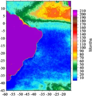
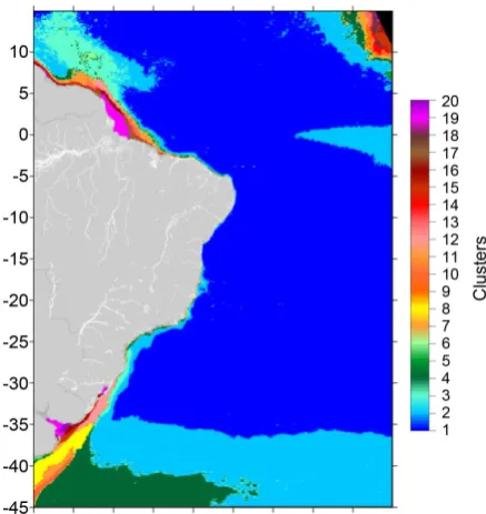
To better show the amount of data to be inferred in the images, which accounts for 11.57% of the total number of pixels, a map was prepared (Figure 2), in which the frequency of the missing data in each pixel is represented in a range of colors. The large purple area is South America, highlighting Brazil, as well as part of the African continent in the upper right corner. A large concentration of missing data in coastal regions and above the equator (zero intercept) is ob-served.

Figure 3 shows the results of the Skill indicator. The Skill for the 5% calcu-lated quantity was 0.8644; 0.8730 for 10%; 0.8830 for 15%, and 0.8904 for 20%. By making a graphical interpolation, it has been estimated that for the case of 11.57% (actual amount of missing data), a Skill of approximately 0.8762 is ob-tained. It is observed that the difference of scenarios between the lowest and the highest Skill is only 2.6%. Also, the actual Skill was estimated at 87.62%, consi-dered extremely high according to several related researches [8] [10] [11] [12] [13] [14] [27] [28].

DOI: 10.4236/jsea.2019.125010 158 Journal of Software Engineering and Applications Figure 2. Map of the study area highlighting the number of missing data by region (9 km between each pixel) in a temporal scale: 0 to 213 months.

Figure 3. Skill for the scenarios and inference for the missing data.

DOI: 10.4236/jsea.2019.125010 159 Journal of Software Engineering and Applications 15%, and 0.6758 for 20%. Similarly, estimating via graphical interpolation for the case of 11.57%, a coefficient of approximately 0.6438 is obtained, and the differ-ence from lowest to highest Coefficient is 5.73%, evaluations also being very close and having an estimated actual coefficient of 64.38%, which is also a high indicator.

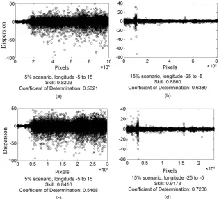
Due to a large number of pixels, a partitioned graphical analysis was per-formed for better qualitative assessment. To conduct such analysis, Figure 2 was observed again and the following areas were selected to compare the dispersion: the geographic region between the longitudes −5 to 15, for having the highest concentration of missing data; and the region between −25 to −5, featuring the lowest concentration. Figure 5 shows the dispersion charts selected for these two regions, being charts Figure 5(a) and Figure 5(b) for the 5% scenario of missing data, and Figure 5(c) and Figure 5(d) for the 15% scenario. For each of them, the Skill and Coefficient of Determination indicators are also presented.

According to the dispersion charts, it can be observed that the proposed algo-rithm has larger differences in the region with the highest amount of missing data, and on the other hand it is very assertive in the region with many observed data. Large dispersions (over 50, for example) do exist, but these are still very few, in a total of more than 3 million pixels. Also, a large concentration of points is observed in the region close to zero, indicating a high level of assertiveness and reliability of results for validation of the objectives proposed by this re-search.

DOI: 10.4236/jsea.2019.125010 160 Journal of Software Engineering and Applications In related studies dealing with data mining of chlorophyll-a concentrations, three points are highlighted as compared to this research [11] [12] [13] [14] [27] [28] [29], namely:

1) Missing data are usually ignored or a pixel is taken as a reference to a larger area, thus being used as a reference for neighboring missing values;

2) Algorithms are used with high computational cost for application in PCs with this large volume of data;

3) The efficiency of estimators for this type of data is typically validated with indicators in the order of 60%.

Therefore, the inference of the actual missing data addressed herein can be considered as efficient, featuring indicators with overall values above 60%, which contributes to a higher resolution in the data mining process and, mainly, enabling the implementation of this procedure with a large amount of data in common computer systems.

3.2. Identifying Patterns in the Atlantic Ocean

The identification of patterns is performed from the clustering process. For these results, four experiments are presented herein:

1) Climatology, with the average of the logs for each month. 2) Climatology, with the complete matrix for each month. 3) Major fields, with the complete matrix for normalized data.

4) Anomalies, with the complete matrix of data, by calculating the anomalies for each pixel.

3.2.1. Climatology

For the construction of the 18-year climatology, two approaches are presented. The first analysis was processed with the natural log average of the concentra-tions for each month, regardless of the year. The input matrix contains 3,510,828 samples with the following features: a latitude-longitude pair, the natural log av-erage of the chlorophyll concentration in a given month, and the month for that average.

With these data, the value of k (clusters or number of centroids) was defined by testing, with details or resolutions being observed as this value varied. Figure 6 shows one of these tests for 20 clusters, Cluster 1 having the lowest average and Cluster 20 the highest average, also having the dynamic behavior well defined for each cluster, which are also away from each other, thus justifying their differen-tiation for analysis purposes. Also for comparison purposes of all the results, the value of k selected for these presentations of results was 20.

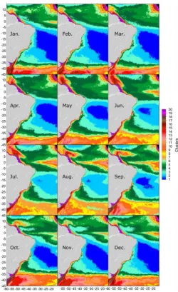
Figure 7 shows the result of this first climatology approach, the clusters being numbered from 1 to 20 according to the oceanographic standard of colors, also ordering the clusters so that Cluster 1 showed the lowest average and Cluster 20 highest one.

DOI: 10.4236/jsea.2019.125010 161 Journal of Software Engineering and Applications Figure 6. Time series variability of clusters centroids obtained from chlorophyll-a concentration.

DOI: 10.4236/jsea.2019.125010 162 Journal of Software Engineering and Applications end, 12 matrices were built, each containing 292,569 lines as a latitude-longitude pair and 17 or 18 columns, representing the months for each year; the result is shown in Figure 8. Unlike the scenario presented in Figure 7, the one represented in Figure 8 has no direct relation between the numbers of each cluster of images for each month, as data mining scenarios were carried out sep-arately.

3.2.2. Overall Concentration

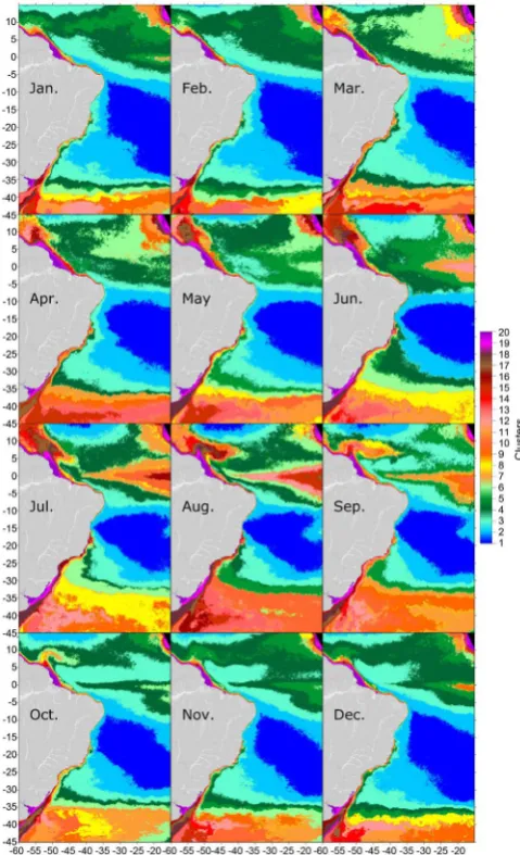
Figure 9 shows the clustering result now considering the complete database (292,569 lines by 213 columns), also with 20 clusters ordered from the lowest to the highest average of the concentration log.

3.2.3. Anomaly

Figure 10 also shows the clustering result now considering the complete data-base (292,569 lines by 213 columns) with 20 clusters, but for the anomaly data that were calculated for each pixel.

DOI: 10.4236/jsea.2019.125010 163 Journal of Software Engineering and Applications Figure 9. Mining with the complete matrix with each month of the chloro-phyll concentration log.

Figure 10. Mining with the complete matrix with each month for anomalies.

3.2.4. Analysis of the Patterns Found

con-DOI: 10.4236/jsea.2019.125010 164 Journal of Software Engineering and Applications centrations found, and during this period, cluster 1 nearly disappears. Also in this period, the largest chlorophyll concentrations in the equator region related to the North Equatorial Current to the east, and the largest development of Re-troflexion of the North-Brazilian Current to the west. During this quarter occurs the largest biological production in the South Atlantic. From October to De-cember, the high production of the southern portion of the South Atlantic (be-low latitude 35˚) stands out, the center portion again has (be-low concentrations, but the equatorial strip still has relatively high concentrations. During this quarter the biggest contrasts between the central and southern portion of the South At-lantic are observed.

Still with respect to Figure 7, clusters 18 through 20 refer essentially to the Amazon region, this region being different from the Atlantic, where the expan-sion and contraction of these clusters throughout the year is observed. In April, the highest concentration of chlorophyll is observed, coinciding with the period of highest rainfall rates, while the lowest concentration is observed in October, coinciding with the dry season. Therefore, in this region, strong influences of the Amazon River itself were detected on these concentrations, probably because of the greater availability of suspended material injected by this river in the ocean. High concentrations are also observed in this region from May through June, which are related to the expansion of the Amazonian Plume.

With respect to Figure 8, in March there occurs a large production of chlo-rophyll where clusters 15 to 18 are identified in the southern part of the map in the confluence between the return of the Brazilian current and the Antarctic Circumpolar Current, emphasizing that this behavior was not observed in Fig-ure 9. So, treating climatology with different metrics and filters is important to identify structures that are not displayed in a single manner. In general, Figure 7 and Figure 8 showed very similar results; however, the month of August is hig-hlighted in Figure 8, when the largest concentrations of chlorophyll and largest extension in the South Atlantic are observed; also, the coastal region of sou-theastern Brazil showed the highest chlorophyll concentrations recorded during the year. This pattern did not appear in Figure 7 either.

DOI: 10.4236/jsea.2019.125010 165 Journal of Software Engineering and Applications in subsequent studies with the spatial distribution patterns of zooplankton and ichthyoplankton, since these may reveal constraints on the spawning and surviv-al of seversurviv-al species of fish and invertebrates.

Finally, Figure 10 shows the clusters formed with anomaly values. This ap-proach allowed for verifying that most of the Atlantic features a major temporal and spatial stability in the variation of chlorophyll concentration (Clusters 1 and 2), thus referring to little variation in annual cycles, since the anomalies, as cal-culated, filter the annual cycles. Near the Amazonian coastline, on the southern stretch of South America and even on the coast of Africa, clusters are made up of higher anomaly values (Clusters 8 to 20); this demonstrates that said regions are subjected to strong inter-annual variations related to the rainfall on the conti-nent that cause large variations in the contribution of chlorophyll in the rivers and, therefore, causing strong influences on the coast.

3.2.5. Computational Assessment

Based on the large volume of data and the notorious computational complexity involved, it can be seen that the methodology described herein can be applied to simple, personal-use computer systems, thus enabling the execution of several tests in short periods of time pointing to reduced costs for related large-scale re-search, without compromising the quality of the results. In this regard, some points of this research will be discussed to better evaluate the experiments that were conducted.

The inference of 7,207,558 pixels recorded as missing data was conducted us-ing 3 computer systems, and the followus-ing results were obtained:

 Ultrabook Positivo, approximately 2 days of processing;

 _{Ultrabook Dell, approximately 5 hours;}  Xeon Server, approximately 8.4 hours.

For the implementation of the 5%, 10%, 15% and 20% scenarios for evaluating the Skill and Coefficient of Determination indicators and the dispersion graphi-cal analysis, as shown in Figures 4-6, the results obtained with the Ultrabook Positivo, the one with lowest performance/hardware, were as follows:

 _{20% of missing data, 12,463,440 pixels, approximately 7 days of processing;}  15% of missing data, 9,347,580 pixels, approximately 5 days of processing;

 _{10% of missing data, 6,231,720 pixels, approximately 4 days of processing;}  5% of missing data, 3,115,860 pixels, approximately 3 days of processing.

Significantly better results were observed by using the Ultrabook Dell and the Xeon Server, respectively, with the MySQL database running on Linux operating system, because of the best RAM, SSD HD and high speed specifications, as well as database memory management and management of the operating system it-self.

Ultra-DOI: 10.4236/jsea.2019.125010 166 Journal of Software Engineering and Applications book Positivo was unable to process in a reasonable amount time (processing interrupted after 7 days of processing). Regarding the smaller matrices, such as the climatology with average values, the Ultrabook Dell completed it in 1 hour, the Xeon Server in 2.5 hours and the Ultrabook Positivo in 24 hours.

4. Discussion

Reference [5] identifies 7 biogeochemical provinces based on chlorophyll-a data within the 45˚S - 5˚N latitude and 15˚W - 60˚W longitude boundaries. These were structured by major oceanographic processes for each region. The results presented herein suggest the presence of 20 clusters for the entire area of study. Thus showing that within the boundaries of each province of [5] there occur more than one mode of chlorophyll-a variability, which vary spatially during the year. This way, according to Figure 9, the following can be identified:

 _{South Atlantic Gyral Province (SATL): 6 clusters.}  _{Western Tropical Atlantic Province (WTRA): 5 clusters.}  Antarctic biome on the west side (SSTC): 9 clusters.

 Guayana coast province (GUIA): 7 clusters.

 _{Coastal province of the Brazilian Current (BRAZ): 4 clusters.}  Tropical North Atlantic Province (NATR): 8 clusters.

Since the clusters identified herein consider the numerical spatio-temporal variability for the entire study area, the clusters identified go beyond the prov-inces identified by [5], thus introducing new areas for research.

The inference of 7,207,558 pixels recorded as missing data was conducted by using the 3 computer systems, the following average processing performances were obtained:

 _{Ultrabook Positivo, approximately 2 days;}  Ultrabook Dell, approximately 5 hours;

 Xeon Server, approximately 8.4 hours.

For the implementation of the 5%, 10%, 15% and 20% scenarios for evaluating the Skill and Coefficient of Determination indicators and the dispersion graphi-cal analysis, as shown in Figures 4-6, the results obtained with the Ultrabook Positivo, with least processing one tested, were as follows:

 _{20% of missing data, 12,463,440 pixels, approximately 7 days of processing;}  15% of missing data, 9,347,580 pixels, approximately 5 days of processing;

 10% of missing data, 6,231,720 pixels, approximately 4 days of processing;

 _{5% of missing data, 3,115,860 pixels, approximately 3 days of processing.}

Significantly better results were observed by using the Ultrabook Dell and the Xeon Server, with the MySQL database running on Linux operating system, given the best RAM, SSD HD and high speed specifications, as well as database memory management and management of the operating system itself.

DOI: 10.4236/jsea.2019.125010 167 Journal of Software Engineering and Applications hours, respectively. However, for these matrices, the Ultrabook Positivo was unable to process in a reasonable amount time (processing interrupted after 7 days of processing). Regarding the smaller matrices, such as the climatology with average values, the Ultrabook Dell completed it in 1 hour, the Xeon Server in 2.5 hours and the Ultrabook Positivo in 24 hours.

In a general context, the modern Ultrabooks, intended for personal use with SSD HD, even if used externally via USB 3.0, and 8 GB RAM, carried out processing satisfactorily, thus contributing to greater popularity of this type of research in this field of application, as they are cheaper computer systems.

Regarding the accuracy of results, the stopping criteria of the k-means is based on the convergence of similarity to a single centroid; the sensitivity of the results presented in the identification of patterns considered 8 decimal places of accu-racy. But it was noted that by increasing to 10 decimal places, for example, the processing time duplicates, thus proving that the simple use of the float or double patterns increase mining time significantly.

The possible analyses of various patterns presented in Figure 7 and Figure 10 while not exhausted here, were identified with high resolution and confirmed re-liability according to the evaluation of the indicators; the analyses had all the missing pixels estimated and accounted for in the mining process. Limitations were also presented with a high amount of missing data, which are also expected in any estimation solution, but the representativeness of these high dispersions in relation to the large volume of data is low.

5. Conclusions

More than one mode of spatiotemporal variability was found for chlorophyll-a concentrations within each biogeochemical province in the Atlantic Ocean. Thus it suggests that the oceanographic processes have a great importance in struc-turing the spatiotemporal variability of chlorophyll-a concentrations; however, they do not act in a homogeneous manner in their spatial domains.

The study area of this research was defined as a large region of the Western Atlantic Ocean, near the Brazilian coast, as far as a part of Africa, totaling more than 60 million records processed in an approach focused on low-cost computer systems.

The clustering with k-means was implemented directly as a function in the database by mapping similar spatiotemporal behaviors, the results of which were presented graphically and analyzed with the climatology of the 18 years period.

The treatment of large volume of missing data is an additional problem for common computers, and the proposed solution with an iterative interpolation algorithm obtained good reliability in the results, especially when comparing the indicators presented herein to several related papers. The patterns identified through data mining will be focus of more specialized analysis in future works.

DOI: 10.4236/jsea.2019.125010 168 Journal of Software Engineering and Applications clustering in regions with similar dynamic behaviors by using low-cost computer systems—was achieved, thus establishing this approach as susceptible to be ap-plied in geographical areas and periods with reduced hardware-related costs.

Recent challenges addressed in this study are highlighted as follows:

1) A missing data inference technique is presented, which can be performed in a computationally efficient form and showing results considered satisfactory by the current literature, with effectiveness greater than 60%.

2) Feasibility for mining large volume of data in the field of oceanography and marine biology by using inexpensive computer systems.

3) The clustering patterns identified can influence new discoveries to scientists in the fields of oceanography and marine biology, also being a tool to be used with other variables estimated by remote sensors available and their correlations; such as sea surface temperature, wind direction and velocity.

Other techniques and tools already directed to large volumes of data can also be tested on PCs and Notebooks for computational performance evaluation in order to further improve the results obtained, such as: Map-Reduce, Hadoop, data stream; and data storage in database managers in NoSQL and NewSQL formats, such as: mongoDB and VoltDB. These techniques, when applied in larger computer systems, can also provide global analyses and correlation of other observable variables effectively.

Conflicts of Interest

The authors declare no conflicts of interest regarding the publication of this pa-per.

References

[1] Field, C.B., Behrenfeld, M.J., Randerson, J.T. and Falkowski, P. (1998) Primary Production of the Biosphere: Integrating Terrestrial and Oceanic Components.

Science,281, 237-240. https://doi.org/10.1126/science.281.5374.237

[2] Kirk, J.T.O. (2011) Light and Photosynthesis in Aquatic Ecosystems. 3rd Edition, Cambridge University Press, Cambridge, England.

[3] Reygondeau, G., Longhurst, A., Martinez, E., Beaugrand, G., Antoine, D. and Maury, O. (2013) Dynamic Biogeochemical Provinces in the Global Ocean. Global Biogeochemical Cycles, 27, 1046-1058.

https://doi.org/10.1002/gbc.20089

[4] Devred, E., Sathyendranath, S. and Platt, T. (2007) Delineation of Ecological Prov-inces Using Ocean Colour Radiometry. Marine Ecology Progress Series, 346, 1-13.

https://doi.org/10.3354/meps07149

[5] Longhurst, A. (2007)Toward an Ecological Geography of the Sea. Academic Press, London. https://doi.org/10.1016/B978-012455521-1/50002-4

[6] Longhurst, A. (1995) Seasonal Cycles of Pelagic Production and Consumption.

Progress in Oceanography, 36, 77-167.

https://doi.org/10.1016/0079-6611(95)00015-1

Post-DOI: 10.4236/jsea.2019.125010 169 Journal of Software Engineering and Applications launch Technical Report Series, SeaWiFS Postlaunch Calibration and Validation Analyses: Part 3, NASA Goddard Space Flight Center, Greenbelt, MD, 9-23. [8] Zhang, Y.-L., et al. (2009) Modeling Remote-Sensing Reflectance and Retrieving

Chlorophyll-a Concentration in Extremely Turbid Case-2 Waters (Lake Taihu, China). IEEE Transactions on Geoscience and Remote Sensing, 47, 1937-1948.

https://doi.org/10.1109/TGRS.2008.2011892

[9] Vilas, L.G., Spyrakos, E. and Palenzuela. J.M.T. (2011) Neural Network Estimation of Chlorophyll a from MERIS Full Resolution Data for the Coastal Waters of Gali-cian Rias (NW Spain). Remote Sensing of Environment, 115, 524-535.

https://doi.org/10.1016/j.rse.2010.09.021

[10] Mcginty, N., Power, A.M. and Johnson, M.P. (2011) Variation among Northeast Atlantic Regions in the Responses of Zooplankton to Climate Change: Not All Areas Follow the Same Path. Journal of Experimental Marine Biology and Ecology, 400, 120-131. https://doi.org/10.1016/j.jembe.2011.02.013

[11] Spyrakos, E., Vilas, L.G., Palenzuela, J.M.T. and Barton, E.D. (2011) Remote Sensing Chlorophyll a of Optically Complex Waters (Rias Baixas, NW Spain): Application of a Regionally Specific Chlorophyll a Algorithm for MERIS Full Resolution Data during an Upwelling Cycle. Remote Sensing of Environment, 115, 2471-2485.

https://doi.org/10.1016/j.rse.2011.05.008

[12] Alameddine, I., Cha, Y.-K. and Reckhow, K.H. (2011) An Evaluation of Automated Structure Learning with Bayesian Networks: An Application to Estuarine Chloro-phyll Dynamics. Environmental Modelling & Software, 26, 163-172.

https://doi.org/10.1016/j.envsoft.2010.08.007

[13] Gaetan, C., Girardi, P. and Pastres, R. (2014) The Role of Spatial Dependence on the Functional Clustering Based on the Smoothing Splines Regression. Proceedings of the METMA VII and GRASPA14 Conference, Torino, 10-12 September 2014, 1-5. [14] Mateu, J. and Romano, E. (2017) Advances in Spatial Functional Statistics.

Stochas-tic Environmental Research and Risk Assessment, 31, 1-6.

https://doi.org/10.1007/s00477-016-1346-z

[15] Nazeer, M. and Nichol, J.E. (2015) Modeling of Chlorophyll-a Concentration for the Coastal Waters of Hong Kong. 2015 Joint Urban Remote Sensing Event, Lau-sanne, 30 March-1 April 2015, 1-4. https://doi.org/10.1109/JURSE.2015.7120460

[16] Zheng, G. and Di Giacomo P.M. (2017) Remote Sensing of Chlorophyll-a in Coastal Waters Based on the Light Absorption Coefficient of Phytoplankton. Remote Sens-ing of Environment, 201, 331-341. https://doi.org/10.1016/j.rse.2017.09.008

[17] Huang, Z. and Wang, X.-H. (2019) Mapping the Spatial and Temporal Variability of the Upwelling Systems of the Australian South-Eastern Coast Using 14-Year of MODIS Data. Remote Sensing of Environment, 227, 90-109.

https://doi.org/10.1016/j.rse.2019.04.002

[18] Djavidnia, S., M’Elin, F. and Hoepffner, N. (2010) Comparison of Global Ocean Colour Data Records. Ocean Science, 6, 61-76.

https://doi.org/10.5194/os-6-61-2010

[19] Giovanni (2019) The Bridge Between Data and Science, Version 4.30, USA.

https://giovanni.gsfc.nasa.gov/giovanni/

[20] Feldman, G.C. (2014) Chlorophyll a (chlor_a). NASA, Ocean Color Web.

https://oceancolor.gsfc.nasa.gov/atbd/chlor_a/

DOI: 10.4236/jsea.2019.125010 170 Journal of Software Engineering and Applications https://doi.org/10.1016/j.jcp.2007.06.016

[22] Macqueen, J. (1967) Some Methods for Classification and Analysis of Multivariate Observations. In: Proceedings of the 5th Berkeley Symposium on Mathematical Sta-tistics and Probability, 1: Statistics, University of California Press, Berkeley, CA, 281-297.

[23] Jain, A.K., Murty, M.N. and Flynn, P. (1999) Data Clustering: A Review. ACM Computing Surveys, 31, 264-323. https://doi.org/10.1145/331499.331504

[24] Xu, R. and Wunsch II, D. (2005) Survey of Clustering Algorithms. IEEE Transac-tion on Neural Networks, 16, 645-678. https://doi.org/10.1109/TNN.2005.845141

[25] Milligan, G.W. and Cooper, M.C. (1987) Methodology Review: Clustering Methods.

Applied Psychological Measurement, 11, 329-354.

https://doi.org/10.1177/014662168701100401

[26] MySQL, Version 8.0.16. (2019) Oracle Corporation, USA.

[27] Irwin, A.J. and Finkel, Z.V. (2008) Mining a Sea of Data: Deducing the Environ-mental Controls of Ocean Chlorophyll. PLoS ONE, 3, e3836.

https://doi.org/10.1371/journal.pone.0003836

[28] Moore, T.S. and Campbell, J.W. (2009) A Class Based Approach for Characterizing the Uncertainty of the MODIS Chlorophyll Product. Remote Sensing of Environ-ment, 113, 2424-2430. https://doi.org/10.1016/j.rse.2009.07.016

[29] Savtchenko, A., Ouzounov, D., Ahmad, S., Acker, J., Leptoukh, G., Koziana, J. and Nickless, D. (2004) Terra and Aqua MODIS Products Available from NASA GES DAAC. Advances in Space Research, 34, 710-714.