Radiation hydrodynamics simulations of the evolution of the diffuse ionized gas in disc galaxies

Radiation hydrodynamics simulations of the evolution of the diffuse

ionized gas in disc galaxies

Bert Vandenbroucke

and Kenneth Wood

SUPA, School of Physics and Astronomy, University of St Andrews, North Haugh, St Andrews KY16 9SS, UK

Accepted 2019 July 2. Received 2019 June 28; in original form 2019 March 15

A B S T R A C T

There is strong evidence that the diffuse ionized gas (DIG) in disc galaxies is photoionized by radiation from UV luminous O and B stars in the galactic disc, both from observations and detailed numerical models. However, it is still not clear what mechanism is responsible for providing the necessary pressure support for a diffuse gas layer at kpc-scale above the disc. In this work, we investigate if the pressure increase caused by photoionization can provide this support. We run self-consistent radiation hydrodynamics (RHD) models of a gaseous disc in an external potential. We find that photoionization feedback can drive low levels of turbulence in the dense galactic disc, and that it provides pressure support for an extended diffuse gas layer. Our results show that there is a natural fine-tuning between the total ionizing radiation budget of the sources in the galaxy and the amount of gas in the different ionization phases of the interstellar medium, and provide the first fully consistent RHD model of the DIG.

Key words: methods: numerical – HIIregions – ISM: structure.

1 I N T R O D U C T I O N

The existence of a diffuse layer of ionized material in our Galaxy

was first proposed by Hoyle & Ellis (1963) to explain an

ob-served absorption feature in the galactic synchrotron background. The existence of this layer was subsequently confirmed through

measurements of its faint Hα emission (Reynolds, Scherb &

Roesler1973); currently large galaxy-wide surveys are available

that provide a full picture of what is now referred to as the warm

ionized medium (WIM) (Haffner et al.2003). Dettmar (1990) and

Rand, Kulkarni & Hester (1990) found similar diffuse ionized layers

in other galaxies, and introduced the general termdiffuse ionized gas

(DIG). The spatial distribution and properties of the DIG have been

extensively studied; see the review by Haffner et al. (2009). The DIG

corresponds to the so calledwarmphase of the interstellar medium

(ISM); the dense disc constitutes acoldphase, while a fraction of

the gas is expected to be in ahotphase at lower densities and higher

temperatures than the DIG (Cox & Smith1974; McKee & Ostriker

1977). For this work, we will only consider the cold and warm

phases of the ISM.

To explain the existence of the DIG, we need to address two important questions:

(i) What mechanism is responsible for ionizing the diffuse gas? (ii) What mechanism is responsible for supporting a diffuse gas layer at the observed heights above the galactic disc?

_{E-mail:[email protected]}

An extensive body of literature exists that addresses the first question. The observed ionization fraction of the DIG can only be explained if the DIG is photoionized by local sources, i.e. UV

luminous O and B stars in the galactic disc (Reynolds et al.1995).

Furthermore, there are strong correlations between the presences of a high star formation rate and the signal from DIG emission

(Rossa & Dettmar 2003), and between line emission from HII

regions surrounding young O stars and DIG emission (Ferguson

et al.1996a). To explain how the UV radiation from these sources

makes it out of the dense galactic disc to the large altitudes where the DIG is observed, we have to assume a turbulent disc structure that

contains low-density channels (chimneys) through which ionizing

radiation can escape (Haffner et al. 2009). Post-processing of

realistic disc models (Joung & Mac Low2006; Hill et al.2012;

Girichidis et al. 2016) has shown that these channels do indeed

exist (Wood et al.2010; Barnes et al.2014; Vandenbroucke et al.

2018, from here onV18).

The temperature of the DIG is typically higher than that in HII

regions in the disc, and tends to increase with altitude above the

disc, both in our Galaxy (Haffner, Reynolds & Tufte1999; Madsen,

Reynolds & Haffner2006) and other galaxies (Ferguson, Wyse &

Gallagher 1996b). Wood & Mathis (2004) showed that such a

temperature structure can be explained by spectral hardening of the radiation field, which is a possible scenario if the sources of ionizing radiation are embedded within a dense molecular cloud

and the DIG is ionized by so calledleakyHIIregions (Hoopes &

Walterbos2003).V18showed that spectral hardening does indeed

produce the expected line emission signature in post-processed disc galaxy models, provided that the UV luminosity of the ionizing sources is fine tuned to reproduce both the scale height of the

2019 The Author(s)

DIG (as measured from the scale height of the Hα profile) and the temperature structure. In these models, the spectral hardening occurs inside the DIG and it is the spectral change throughout the DIG that reproduces the observed increase in line emission. Note that the observed temperature structure of the disc can also be explained by considering the impact of hot evolved stars (Rand

et al. 2011; Flores-Fajardo et al. 2011), and that a full model

for the DIG should also take into account other sources of UV radiation.

Models of the DIG until now have failed to address the second question. Those attempts that post-processed realistic disc galaxy models were dependent on the specific model feedback implemen-tations to explain the presence of diffuse gas in these models; when a diffuse component is present, it can be ionized and produces a realistic DIG. However, models without sufficient diffuse gas at

high altitudes are less satisfactory (Barnes et al.2014,V18). Clearly,

some mechanism is required to provide pressure support for diffuse gas at high altitudes.

In this paper, we build on the correlation found between the

ionizing source luminosity and the scale height of the DIG inV18,

and propose that photoionization itself is responsible for producing the necessary pressure support to maintain the DIG. Neutral atomic gas has a typical temperature of 100–500 K, while gas in the DIG

has an equilibrium temperature of∼8000 K and more. This increase

in temperature gives the DIG a significantly higher hydrodynamic pressure, which provides extra support against the gravitational potential of the disc. We know that the ionizing radiation has to make it out to the high altitudes where the DIG is supported, so this mechanism will be effective at these altitudes.

To quantify this effect, we will run idealized radiation hydrody-namics (RHD) simulations of a patch of a disc galaxy that is initially in ionized hydrostatic equilibrium in an external disc potential. We will then add a realistic distribution of luminous O stars to this setup and study how the UV radiation of these sources affects the dynamics of the gas in the disc. We post-process these simulations

using the same model as employed inV18 (and using the same

number of sources and source positions as in the corresponding RHD model), and verify that this still produces a DIG that is in line with the observed DIG. To our knowledge, this is the first self-consistent RHD study of the DIG; previous models of ionized gas in disc galaxies focused on the central galactic disc (de Avillez et al.

2012; Seifried et al.2017) and did not study the impact of radiation

on the extended diffuse disc.

The paper is structured as follows: first, we will introduce our method. We will then show that our models give converged results, and discuss the effect of our model parameters on the results. We will end with our conclusions.

2 M E T H O D

Full radiation transfer modelling of the DIG and all relevant cooling and heating mechanisms is computationally expensive. We will therefore employ a two-step technique to model the dynamics of the DIG and the resulting DIG structure:

(i) first, we will run RHD models in which the radiation field is treated using a simplified two-temperature model with hydrogen as

the only absorber of ionizing radiation (Lund et al.2019,

Falceta-Gonc¸alves et al., in preparation),

(ii) then, we will post-process these simulations to produce a more complete model of the temperature structure and ionization

state, using the fullV18model. Note that these models are only

intended to check that the spectral hardening found inV18is still

effective, and not to produce a full spectral model for the DIG.

For both steps, we will use the Monte Carlo RHD code CMACIONIZE1 (Vandenbroucke & Wood2018a,b), both in its full RHD mode and its post-processing mode. For consistency, we will use the same grid and source model for the RHD step and the post-processing step.

Below we discuss both models and our initial conditions in more detail.

2.1 RHD model

2.1.1 External potential

We will assume that the total mass contained in the gas in our simulations is only a small fraction (10 per cent) of the total mass budget, so that we will approximate the gravitational potential with an external, analytic potential. To this end, we use the same isothermal sheet potential used by the SILCC project (Walch et al.

2015), with the gravitational accelerationagravgiven by

agrav= −2πGMtanh

z bM

, (1)

withzthe altitude above the plane of the disc andG=6.674×

10−11_m3_kg−1_s−2_{Newton’s constant. The two parameters for the}

potential are the surface densityMand the scale heightbM, for

which we will use the same values as used for SILCC: M=

30 Mpc−2_{andbM=200 pc.}

Creasey, Theuns & Bower (2013) parametrize the isothermal

sheet potential in terms of the gas surface densityg=fgM, with

fgthe fraction of the total mass that is in gas (we assumefg=0.1).

Assuming that the gas has the same density distribution as the other mass components, they find an expression for the gas scale height

bg(=bM) for gas in hydrostatic equilibrium with the potential at

temperatureT:

bg= fgkBT μmpπGg ≈

611 μ T 1000 K M

1 Mpc−2

−1

pc, (2)

withkB=1.38064852×10−23_{J K}−1_{Boltzmann’s constant,mp=}

1.6726219×10−27_{kg the mass of a proton, and μ the mean}

molecular weight of the gas. The SILCC choice of parameters hence

corresponds to a neutral hydrogen only gas atT ≈104_K.

In Section 2.2, we will discuss the density distribution that corresponds to this potential.

2.1.2 Equation of state

We will assume a two-temperature isothermal equation of state for

the gas, with the pressurePgiven by

P = ρkBTeq

μeqmp, (3)

withρthe gas density andTeqandμeqthe equilibrium temperature

and mean molecular mass, given by

Teq=xHTn+(1−xH)Ti, (4)

and

μeq=xH+1

2(1−xH)=

1

2(xH+1), (5)

1_{https://github.com/bwvdnbro/CMacIonize}

withxHthe neutral fraction of hydrogen for a cell. The two

tempera-turesTnandTicorrespond to the assumed equilibrium temperatures

for neutral and ionized gas respectively. We will assumeTn=500 K

andTi=8000 K. Note that we choose a relatively high neutral gas

temperature to account for the fact that we do not include any additional feedback processes: at lower temperatures our density profile becomes very steep and it is very hard for the radiation to create outflow cavities through which ionizing radiation escapes into the diffuse disc. In the presence of additional feedback mechanisms, we would expect these cavities to be present and facilitate the escape of ionizing radiation.

2.1.3 Radiation

To simplify the radiation transfer during the RHD simulations, we will assume a monochromatic ionizing spectrum with an

energy of 13.6 eV, and a constant photoionization cross-section of

6.3×10−18_cm2_{(since the photon energy only affects its}

photoion-izing cross-section in this problem, the use of a monochromatic spectrum is not strictly necessary). We furthermore assume a

constant recombination rate of 2.7×10−13_cm3_s−1_{. This implies}

a recombination time-scaletR=1.2×105_nH/cm−3−1_yr.

De-pending on the resolution, we use 107_{or 10}8_{photon packets per}

iteration for 10 iterations. To limit the impact of the radiation step on the integration, we do not do the full radiative transfer calculation after every hydrodynamical integration step, but instead update the ionization state on a regular time interval basis. We run simulations

with radiation intervals of 0.1, 0.5, and 1 Myr. We will show the

effect this has on our final result below.

As an ionizing source model, we will use the same distribution as

used inV18, with uniform random coordinates in the plane of the

disc, and a Gaussian vertical distribution perpendicular to the disc, with a scale height of 63 pc. We assume an average source number

density of 24 kpc−2and an average source lifetime of 20 Myr. The

ionizing luminosity per source,QH, is a parameter in our model;

we will explore three different values: 1047_{, 10}48_{, and 10}49_s−1_.

These values correspond to respectively 1 per cent, 10 per cent, and 100 per cent of the ionizing luminosity of an average O/B star, and take into account the fact that we do not resolve the dense birth clump of these stars which can be expected to absorb a significant fraction of the ionizing radiation. To limit the number of parameters in our model, we assume the same ionizing luminosity per source and ignore variations because of stochastic sampling of the initial mass function.

We keep track of the lifetime of each individual source, and allow for the creation and destruction of sources over time. To this end, we start by sampling 24 source positions at the start of the simulation, and give each source a lifetime sampled from

a uniform distribution in [0,20] Myr. At regular intervals (we

use a value 1 Myr corresponding to the longest time between radiation steps in all our simulations), we remove sources whose lifetime was exceeded (we currently ignore any impact of supernova feedback at the end of a source lifetime). We then check for the potential creation of new sources: we draw 24 random numbers and for each of them check if they are larger or smaller than the

source creation probability (1 Myr)/(20 Myr)=5 per cent. For each

random number that is smaller, we create an additional source with a lifetime of 20 Myr that is uniformly offset within the 1 Myr interval.

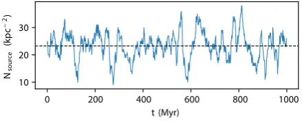
Fig.1shows the resulting number of sources as a function of time.

Note that we keep the source distribution fixed for all our models and only vary the ionizing luminosity of each individual source.

Figure 1. Number of ionizing sources,Nsource, as a function of time for

one of our simulations. Note that our source model ensures that this curve is the same for all simulations. The black dashed line indicates the integrated average.

Note that we do only include the effect of sources in the disc, and do not consider the impact of hot evolved stars, as done in e.g.

Rand et al. (2011) and Flores-Fajardo et al. (2011). The reason for

this is that the total ionizing luminosity of O/B stars is significantly

higher than that of hot evolved stars: Flores-Fajardo et al. (2011)

find an ionizing luminosity QH=7.8×1053_s−1 _{for the former}

and QH=2.1×1051_s−1 _{for the latter. The ionizing luminosity}

of hot evolved stars is hence only a few per cent of that of the

more luminous sources in the disc, even if only∼10 per cent of

the O/B star luminosity makes it out of the unresolved birth cloud surrounding it. Additionally, the O/B star luminosity is significantly more concentrated in space. The appearance and disappearence of a small number of O/B stars will hence have a much more significant dynamical impact than the gradual changes in a diffuse and more extended distribution of hot evolved stars.

Despite their relatively small dynamic effect, hot evolved stars will contribute to the heating of the DIG, as the harder spectrum of these sources can penetrate the diffuse gas more easily. A fully self-consistent model for the spectral emission from the DIG should therefore include these sources; we choose to focus on the impact of O/B stars alone in this work.

2.1.4 Simulations

We sample a slice of the disc in a box of 1×1×8 kpc with

periodic boundaries in thex-andy-directions and semipermeable

boundaries in the z-direction (we allow material to leave the

box, but we do not allow material to enter). We find that these semipermeable boundaries are necessary to prevent unrealistically large inflows through the boundaries. We run simulations at two

different resolutions: 64 × 64 ×512 and 128 × 128 ×1024

cells, corresponding to a spatial resolution of 15.6 and 7.8 pc,

respectively. Due to computational limitations, we will only run one high-resolution simulation and use that to assess the impact of resolution; we will not attempt to obtain spatially converged results. All simulations were run for a total time of at least 800 Myr, with a global time-step set by the hydrodynamical stability condition (we use a CFL factor of 0.2). The high-resolution simulation was only run for 200 Myr. The hydrodynamics scheme is the

same as described in Vandenbroucke & Wood (2018b), with

some minor modifications to deal with numerical issues resulting from the very low densities at high altitudes above the disc in the presence of an external acceleration due to the gravitational potential: a conservative flux limiter that suppresses unrealistically large gravitationally driven mass fluxes, and a velocity limiter that

artificially limits the fluid velocity and sound speed to 1000 km s−1.

We find that these modifications have no noticeable impact on the

Figure 2. Value of the functionI(x) for a realistic range of scale height ratiosx. The full line represents the numerically evaluated value, while the dashed line is a four-parameter fit, as indicated in the legend.

Table 1. Values for the fit parameters in Fig.2.

A 0.015

B −0.085

C 0.635

D −0.010

result of our simulations, but are necessary to maintain stability. The hydrodynamical fluxes are computed using an approximate HLLC Riemann solver.

2.2 Initial conditions

As initial conditions, we assume an ionized hydrogen gas (T =

Ti=8000 K) in hydrostatic equilibrium with the external potential.

Since our initial gas temperature is not the same as the assumed equilibrium temperature used to determine the scale height for the potential, we cannot use the density profile from Creasey et al.

(2013), but instead we need to use the more general expression

ρ=

g

2bM

sech

z bM

2bM

bg

. (6)

In the specific casebg=bM, we recover the density profile used by

Creasey et al. (2013).

The gas surface density_gnow has the more general form

_g=I(bM/bg)fgM, (7)

with

I(x)=2

_+∞

−∞ sech 2x

(y) dy

−1

. (8)

This expression can be derived by imposingMg=fgMM, whereMg

andMMare the total gas mass and total mass within an infinitely

high box.

The integralI(x) has no general analytic solution. We compute it

numerically for a large range ofxvalues and interpolate on these

to get its value for arbitrary scale height ratios. The value ofI(x)

and our interpolating curve are shown in Fig.2and Table1. For

small-scale height ratios (bglarger thanbM), the gas mass is more

spread out than the total mass and the gas surface density is lower

thanfgM. For large ratios (smallbg), the surface density is higher,

reflecting a more concentrated gas density profile.

The initial density profile is plotted in Fig.3for different values of

the initial equilibrium temperatureT0. Note that for realistic neutral

gas temperatures∼100 K the density profile is relatively steep and

has a lower scale height than found in models that employ a detailed

supernova feedback model (Girichidis et al.2016). This indicates

that detailed feedback modelling provides additional heating that

Figure 3. Equilibrium hydrostatic density profile for three different values of the equilibrium temperatureT0(as indicated in the legend) and a fixed gas

surface densityg=2 Mpc−2_{. For reference, we also plot the average}

density for one of the simulations with only thermal feedback of Girichidis et al. (2016). The bottom panel shows a zoom on the central part of the top panel.

increases the average temperature in the disc. For our assumed

neutral temperatureTn=500 K, we find a central density profile

that is more similar to a supernova-supported disc. Since we do not include any other feedback mechanisms apart from photoionization feedback, we will use this temperature as our assumed neutral temperature in the two-temperature equation of state to mimick the dynamical effect of supernova feedback.

For an equilibrium temperature of 8000 K, the scale height of the density profile increases significantly. This already indicates that the temperature increase caused by photoionization can indeed lead to a more extended, diffuse gas component, provided that enough radiation makes it out of the disc to ionize out to sufficiently high altitudes.

Note that the absence of supernova feedback injection will affect the amount of turbulence in our disc, and hence the creation of chimneys through which ionizing radiation can escape. These chimneys will need to be created by photoionization. Our somewhat higher assumed neutral temperature should aid this process. None the less, this means we cannot expect to constrain the ionizing

source luminosityQHwith these models, and hence treat it as a

parameter.

Finally, our choice to start with a fully ionized gas atTi=8000 K

could also affect our results. We will test the impact of this choice by comparing with a simulation that starts with a fully neutral gas

atTn=500 K.

2.3 Post-processing

The post-processing step is very similar to the full model used in

V18. We assume the same abundances for hydrogen, helium, and

all coolants, i.e. He/H=0.1, C/H=1.4×10−4_{, N/H=6.5×10}−5_,

O/H=4.3×10−4_{, Ne/H=1.17×10}−4_{, and S/H=1.4×10}−5_. We also use the same ionizing source spectrum corresponding

to a 40,000 K star with a surface gravity of log (g/(m s−1_{)) =}

3.40. However, we now will use the source positions and ionizing

luminosityQHthat was also used for the RHD step, for consistency.

The RHD step already uses a regular Cartesian grid; we will use the same grid for the post-processing step.

Since the resolution of our simulations is similar to that inV18,

we will use similar Monte Carlo parameters: 108_{photon packets for}

20 iterations.

To test the impact of an additional distribution of hot evolved stars on our results, we will run two additional post-processing simulations for our reference model with an ionising source

lumi-nosity ofQH=1048_s−1_{. These simulations include an additional}

smooth distribution of hot stars, with a total ionizing luminosity of

1048_s−1_{(∼5 per cent of the total ionizing budget in the simulation).}

We assume a flat ionizing spectrum between 1 and 4 Ryd, and furthermore assume a Gaussian distribution. Model ES1 assumes a scale height of 200 pc for the additional sources (consistent with the assumed gravitational potential), while model ES2 has a scale height of 400 pc. For these simulations, we double the number of

photon packets; the extra 108_{photon packets are used to sample the}

additional component (with a lower weight per photon packet).

3 R E S U LT S A N D D I S C U S S I O N

3.1 Convergence

3.1.1 Resolution

Before we can discuss the physical results of our simulations, we have to make sure we understand how our adopted numerical

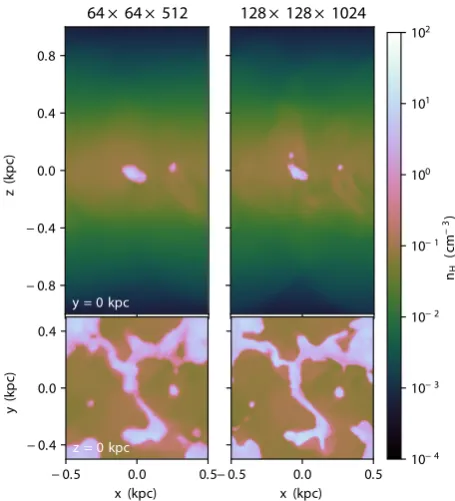
resolution affects our results. Fig.4 shows the density structure

Figure 4. Density slices through simulations with two different resolutions, as indicated in the titles. The top row shows slices along the planey=

0 kpc, while the bottom row shows slices along the planez=0 kpc. Both simulations are shown after 200 Myr of evolution.

Figure 5. Average density as a function of altitude above the disc (z) for simulations with different numerical resolutions, as indicated in the legend. For reference, we also show the hydrostatic equilibrium curves for the neutral and ionized temperatures as black curves. Both simulations are shown after 200 Myr of evolution.

of the disc after 200 Myr of evolution, for two simulations that only differ in the numerical resolution that was used. The density structures look overall similar, but the higher resolution simulation shows more small-scale features that are not resolved in the low-resolution version.

The average density profiles for both runs are shown in Fig.5.

Overall, the density profiles are in good agreement; our low-resolution simulations can be considered to be converged for our purposes.

3.1.2 Radiation time-step

Fig.1shows the number of discrete sources as a function of time for

all of our models. The average number of sources is∼23.3, close to

the target number of 24, but there is some scatter around this value that happens on short time-scales.

This scatter, together with the dynamical effect of the radiation, will change the way the radiation interacts with the ISM over time. In Section 2.1.3, we mentioned that updating the ionization state of the gas in the simulation after every hydrodynamical time-step would be too expensive, and that we only do the radiation step after a fixed time interval. Here, we check what the effect of this approximation is on our final result.

Fig.6shows the density profile for the three different radiation

time-steps after 800 Myr of evolution. The three profiles are in good agreement over most of the range and only diverge in the low-density outskirts.

Fig.7shows slices through the density structure for the same

models. These are also in excellent agreement; the only noticeable differences are some small-scale features that are caused by a lack of time resolution for the models with a longer radiation time-step. Since we are mainly interested in the large-scale structure of the

DIG, we conclude that using a radiation time-steptrad=0.5 Myr

is sufficient to get representative results.

3.1.3 Initial gas temperature

A final model choice that could have a significant impact on our results is the initial ionization state and temperature of the gas. As pointed out in Section 2.2, the neutral hydrostatic density profile is very steep, leading to very low values of the density at high

Figure 6. Average density as a function of altitude above the disc (z) for simulations with three different values of the radiation field update time-step

trad, as indicated in the legend. For reference, we also show the hydrostatic

equilibrium curves for the neutral and ionized temperatures as black curves. All simulations are shown after 800 Myr of evolution.

Figure 7. Density slices through the simulations with different values of the radiation time-steptrad, as indicated in the titles. The top row shows

slices along the planey=0 kpc, while the bottom row shows slices along the planez=0 kpc. All simulations are shown after 800 Myr of evolution. altitudes above the disc. This leads to numerical problems, as the density values reach values very close to the numerical precision of a double precision floating point variable. This explains our choice for a default ionized initial condition that has a better numerical behaviour.

But this choice has profound implications for the dynamics of the simulation. For sufficiently low values of the ionizing luminosity per source, we expect to obtain a gas with two distinct phases: an ionized and a neutral phase. Since the initial condition corresponds to a single one of those phases, there will be an initial adaptation phase during which the initial gas converts part of its gas into the appropriate second phase. This will lead to a large-scale relaxation

Figure 8. Density slices through the simulations with different initial conditions for the gas, as indicated in the titles. The top row shows slices along the planey=0 kpc, while the bottom row shows slices along the planez=0 kpc. All simulations are shown after 800 Myr of evolution.

Figure 9. Average density as a function of altitude above the disc (z) for simulations with different initial conditions for the gas, as indicated in the legend. For reference, we also show the hydrostatic equilibrium curves for the neutral and ionized temperatures as black curves. All simulations are shown after 800 Myr of evolution.

flow in the box. If we start with an ionized initial condition, then the relaxation flow will be directed inwards: the lack of neutral phase leads to an average gas temperature that is lower than the assumed equilibrium and cold gas will fall towards the centre of the gravitational potential. For a neutral initial condition, the reverse happens, and warm gas is expelled from the central disc.

Fig.8shows the density structure for the two different initial

condition scenarios after 800 Myr of evolution. The two simulations are in good agreement, illustrating that by this time, a steady-state equilibrium is reached for the central part of the disc that is independent of the initial condition. This can also be seen in the

average density profiles in Fig.9: the central density profiles agree

very well. The difference in large-scale relaxation flow is however

Figure 10. Average density as a function of altitude above the disc (z) for simulations with three different values of the ionizing luminosityQH,

as indicated in the legend. For reference, we also show the hydrostatic equilibrium curves for the neutral and ionized temperatures as black curves. All simulations are shown after 800 Myr of evolution.

Figure 11. Histograms of the ionized gas fraction for simulations with three different values of the ionizing luminosityQH, as indicated in the legend.

Only the cells with|z|<2 kpc are shown, since cells at higher altitudes only contribute to the lowest bin. All simulations are shown after 800 Myr of evolution.

still apparent from the average density at higher altitudes, which is significantly higher for the neutral initial condition, consistent with a relaxation flow that is directed outwards.

3.2 Ionizing luminosity

For this work, we will assume that our external potential and equation of state are fixed, so that our model is entirely determined by the parameters of the ionizing source model. Since the number of ionizing sources and their scale height has been chosen based on observations, there is only one free parameter in our model: the

ionizing luminosity for an individual source,QH.

Fig.10shows the average density as a function of altitude above

the disc for three different values of the ionizing luminosityQH. It

is clear that higher values of the ionizing luminosity lead to overall higher average densities for the diffuse gas, and lower densities for the neutral disc, as gas is converted from being in a quasi-hydrostatic neutral state into a quasi-quasi-hydrostatic ionized state. This

is even more evident from the histograms shown in Fig.11that show

the number of cells with a given neutral fraction for hydrogen,xH:

as the ionizing luminosity increases, the number of cells within the (partially) neutral bins decreases, and more cells enter the highly

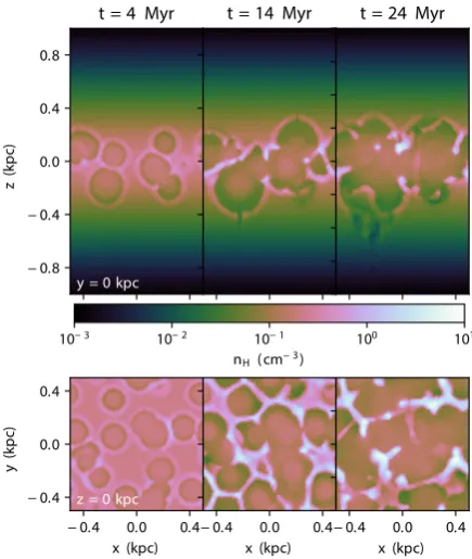
Figure 12. Three snapshots of the time evolution of the ionized bubbles in the early phases of the same simulation, showing the compression of the gas in regions where multiple bubbles collide. The simulation shown is the low-resolution reference model with an ionizing luminosityQH=1048s−1

and radiation time-steptrad=0.5 Myr.

ionized bin. Note also the clear separation between the ionized and the neutral state in these histograms.

That the gas is not actually in strict hydrostatic equilibrium is clear from the tails of the average density profiles: all of the models have an extended tail that lies above the expected hydrostatic equilibrium curve. This corresponds to gas that is either outflowing or is falling back to the centre of the gravitational potential after being previously expelled. This behaviour is to be expected, as the source model itself is constantly evolving and causing small-scale movements of the gas.

There are a number of explanations for the increasing conversion from neutral gas in the central disc to ionized gas in the diffuse disc with increasing ionizing luminosity. As can be seen from the

early evolution of one of our models in Fig.12, the central density

structure is predominantly governed by the interaction of expanding ionization bubbles surrounding the individual ionizing sources. These bubbles collide as they expand and gas in the resulting shock fronts is compressed into dense structures that are hard to ionize. At the same time, the part of the ionizing shell that expands in the vertical direction carries dense gas with it and expels it into the diffuse ionized layer. Higher ionizing luminosities lead to ionization bubbles that expand faster and hence more expelled material and denser structures in the disc plane. In the extreme case of a very high ionizing luminosity, the dense structures in the disc plane can still be ionized effectively and no neutral gas is left.

3.3 Line emission

Thus far, we have only discussed the density structures that result from our RHD simulations. We will now post-process the models with different values for the ionizing luminosity using the same

Figure 13. Line emission maps for (from top to bottom): neutral hydrogen, Hα, [NII]/Hαand [SII]/Hαfor the low-resolution simulations with different values of the ionizing luminosity. All simulation results were obtained by post-processing the output of the different simulations att=800 Myr, as shown in Fig.10.

model as was used forV18, to compute a more detailed temperature

structure and line emission strengths. Note that we use the same source positions and ionizing luminosities that were used during the RHD simulation, so that our model is self-consistent. This is

a significant improvement overV18, where the source positions

were chosen randomly and had no link to the spatial locations of feedback events in the underlying SILCC model. Also recall that these models are not intended to provide a full spectral model for the DIG; we are only quantifying the impact of ionizing radiation from O/B stars in the disc on the spectral properties of the DIG.

Fig. 13 shows line emission maps for the main tracers of the

neutral and ionized gas in our discs for different ionizing source luminosities. All of these were created by integrating the

contri-butions of individual cells along they-direction. It is immediately

clear that the highest luminosity result lacks any clear neutral disc. The neutral disc in the other two simulations shows clear structures of outflows driven by expanding and contracting photoionization bubbles which look similar to observed Milky Way features (Heiles

1984; Koo, Heiles & Reach1992; Hartmann & Butler Burton2012),

as well as clear signatures of active HIIregions in the disc (these

show up as bright spots in Hα), similar to e.g. the Galactic maps from

the WHAM survey (Haffner et al.2003). For the simulations with

Figure 14. Profiles of the neutral hydrogen, Hαintensity, and Hβintensity as a function of height above the disc for the low-resolution simulations with different values of the ionizing luminosity, as indicated in the legend. The full lines correspond to the average values for lines of equal z in Fig.13, while the shaded regions represent the standard deviation over the same lines (these are asymmetric on the panels with a logarithmicy-axis). All simulation results were obtained by post-processing the output of the different simulations att=800 Myr, as shown in Fig.10.

a neutral disc, we see a clear trend in the [NII]/Hαand [SII]/Hα

line ratios: these tend to increase towards higher altitudes above the disc.

The corresponding emission profiles for all simulations are shown

in Figs14and 15. These profiles were created by averaging the

emission maps in Fig.13 overallx-directions. The Hαemission

increases with increasing ionizing luminosity, while the neutral

hydrogen has the opposite trend. Note that the Hα emission is

relatively low compared to that in the observed DIG, indicating that our diffuse gas densities are too low. This might be explained by the absence of strong supernova feedback in our simulations, or by the fact that we do not take into account the fluorescence of the Lyman

lines (Flores-Fajardo et al.2011). Also note that the high luminosity

curve has almost no scatter, indicative of the fact that all the gas in this simulation is highly ionized.

Fig.15also shows the impact of an additional hot evolved star

component in ourQH=1048_s−1_{reference model. This additional}

component has a negligible impact on the neutral gas fractions and

Hαand Hβemission, and very little impact on the [SII]/Hαratio.

It does lead to a noticeable shift in the [NII]/Hα ratio at higher

altitudes, indicative of a shift from N+to N++as dominant nitrogen

ion. This is mirrored in the ionization structure of oxygen, with

a clear increase of the [OIII4959+5007 Å]/Hβline ratio. The

line ratio of [NeIII15μm]/[NeII12μm] is affected most by the

additional evolved star component: while the original models have a slowly increasing ratio as a function of height, consistent with the

Rand et al. (2011) observations, the additional component boosts

Figure 15. Line ratios for [NII]/Hα, [SII]/Hα, [OIII]/Hβ, and [NeIII]/[NeII] as a function of height above the plane of the disc, for the same simulations shown in Fig.14. We also show the results for two additional models (ES1 and ES2) that use a source luminosityQH=1048s−1 and

assume an additional hot evolved stellar component with an ionising luminosity of 1048s−1with a scale height of 200 and 400 pc.

this ratio by two orders of magnitude. This is consistent with the

results for neon found in Flores-Fajardo et al. (2011).

Fig.16shows the relative strength of the forbidden line emission

from [NII] 6584 Å and [SII] 6725 Å as a function of the Hαemission

strength. The models with low luminosities reproduce the observed sulfur line ratio trend; the intermediate luminosity even matches the observed values. The high luminosity result has much lower line ratios than observed, again indicative of its unrealistic ionization structure. For the nitrogen line ratios, the correspondence is less, but we can still see a similar trend in the low-luminosity results. It

is important to note that our models ignore Lyαfluorescence and

therefore underestimate the total Hαluminosity.

The line ratios still depend on the ionizing luminosity, but

unlike in V18, this now can be linked to the dynamic effect of

photoionization: luminosities that are too high ionize too much gas. This does not only lead to line ratios that are lower than observed, but also to a DIG structure that is denser than observed, and the

complete absence of a neutral disc. As inV18, luminosities that are

too low lead to realistic line ratios, but fail to support any significant DIG. We conclude that the observed line ratios are indicative of effective spectral hardening throughout the DIG (as can be seen

in the temperature profiles inV18), and that such a signature is a

natural consequence of the DIG being supported by the increase in temperature caused by photoionization. Furthermore, our O/B star only model agrees well with observed line ratio trends; an additional hot evolved star component with a much harder spectrum has little impact, and fails to reproduce the observed neon line ratio.

4 C O N C L U S I O N S

In this work, we have presented the first self-consistent RHD simulations of the DIG in disc galaxies. We show that a fully self-consistent treatment of photoionization as part of the dynamical modelling of a disc galaxy slab naturally leads to a diffuse ionized disc component that is supported by photoionization heating. This layer has a temperature structure that is in line with observed

Figure 16. Line ratios of the forbidden nitrogen and sulfur lines as a function of the Hαemission for our low-resolution models with different values for the ionizing luminosity and the two additional models with a hot evolved star component, as indicated in the legend. The full lines denote the average line ratio within 50 logarithmic bins, while the shaded regions represent the standard deviation within these bins. The dashed line is the sensitivity limit of the Wisconsin Hαmapper and is indicative for the range that is accessible in observations. The dots represent reference observational data from the WHAM survey (Haffner et al. 1999). Hα intensities are quoted in Rayleigh to facilitate comparison with the WHAM observations. All simulation results were obtained by post-processing the output of the different simulations att=800 Myr, as shown in Fig.10.

DIG properties, provided that the ionizing luminosity is sufficiently strong to support a DIG, and weak enough to allow for the existence

of a neutral disc. The fine-tuning found in previous work (V18) is

hence naturally explained by the dynamic impact of photoionizing radiation.

Despite being very basic, our models are relatively expensive, forcing us to make strong assumptions about the coupling between radiation and hydrodynamics. This means that we cannot currently constrain the properties of the ionizing radiation field, nor make strong predictions about the actual temperature structure of the DIG that would result from an observed distribution of sources, nor provide a full spectral model of the DIG that explains all observed line ratios. Nevertheless, our models provide a valuable insight into the close link between the dynamical effect of photoionizing radiation and the observed properties of the DIG.

The diffuse gas in our models is generally more diffuse than that in the observed DIG. This indicates that (i) the DIG is not in hydrostatic equilibrium, as our densities are close to the expected hydrostatic equilibrium values, but is instead either outflowing or being accreted, and (ii) we are missing additional feedback energy that provides extra support or drives strong outflows that boost the density in the diffuse component. Supernova feedback is one

clear missing feedback mechanism (Walch et al.2015); additional

mechanisms like cosmic ray feedback (Girichidis et al. 2016) or

magnetic fields (Hill et al.2012) can be included as well. A full

quantitative model for the DIG should also contain more realistic

stellar luminosities, lifetimes, and spectra, and a more physically motivated source distribution model that places UV sources in dense neutral clumps and that includes photoionizing radiation from hot evolved sources. All of these can be addressed in future work to provide a more realistic model that will enable more detailed comparisons with observations.

AC K N OW L E D G E M E N T S

We thank Alex S. Hill for comments that improved the quality of this work. BV and KW acknowledge support from STFC grant ST/M001296/1. Part of this work was performed using the DiRAC Data Intensive service at Leicester, operated by the University of Leicester IT Services, which forms part of the STFC DiRAC

HPC Facility (www.dirac.ac.uk). The equipment was funded by

BEIS capital funding via STFC capital grants ST/K000373/1 and ST/R002363/1 and STFC DiRAC Operations grant ST/R001014/1. DiRAC is part of the National e-Infrastructure.

R E F E R E N C E S

Barnes J. E., Wood K., Hill A. S., Haffner L. M., 2014,MNRAS, 440, 3027 Cox D. P., Smith B. W., 1974,ApJ, 189, L105

Creasey P., Theuns T., Bower R. G., 2013,MNRAS, 429, 1922

de Avillez M. A., Asgekar A., Breitschwerdt D., Spitoni E., 2012,MNRAS, 423, L107

Dettmar R.-J., 1990, A&A, 232, L15

Ferguson A. M. N., Wyse R. F. G., Gallagher J. S. III, Hunter D. A., 1996a, AJ, 111, 2265

Ferguson A. M. N., Wyse R. F. G., Gallagher J. S., 1996b, AJ, 112, 2567 Flores-Fajardo N., Morisset C., Stasi´nska G., Binette L., 2011,MNRAS,

415, 2182

Girichidis P. et al., 2016,ApJ, 816, L19

Haffner L. M. et al., 2009,Rev. Mod. Phys., 81, 969

Haffner L. M., Reynolds R. J., Tufte S. L., 1999,ApJ, 523, 223

Haffner L. M., Reynolds R. J., Tufte S. L., Madsen G. J., Jaehnig K. P., Percival J. W., 2003,ApJS, 149, 405

Hartmann D., Butler Burton W., 2012, Atlas of Galactic Neutral Hydrogen. Cambridge Univ. Press, Cambridge

Heiles C., 1984,ApJS, 55, 585

Hill A. S., Joung M. R., Mac Low M.-M., Benjamin R. A., Haffner L. M., Klingenberg C., Waagan K., 2012,ApJ, 750, 104

Hoopes C. G., Walterbos R. A. M., 2003,ApJ, 586, 902 Hoyle F., Ellis G. R. A., 1963,Aust. J. Phys., 16, 1 Joung M. K. R., Mac Low M.-M., 2006,ApJ, 653, 1266 Koo B.-C., Heiles C., Reach W. T., 1992,ApJ, 390, 108

Lund K., Wood K., Falceta-Gonc¸alves D., Vandenbroucke B., Sartorio N. S., Bonnell I. A., Johnston K. G., Keto E., 2019,MNRAS, 485, 3761 Madsen G. J., Reynolds R. J., Haffner L. M., 2006,ApJ, 652, 401 McKee C. F., Ostriker J. P., 1977,ApJ, 218, 148

Rand R. J., Kulkarni S. R., Hester J. J., 1990,ApJ, 352, L1

Rand R. J., Wood K., Benjamin R. A., Meidt S. E., 2011, ApJ, 728, 163

Reynolds R. J., Scherb F., Roesler F. L., 1973,ApJ, 185, 869

Reynolds R. J., Tufte S. L., Kung D. T., McCullough P. R., Heiles C., 1995,

ApJ, 448, 715

Rossa J., Dettmar R.-J., 2003,A&A, 406, 493 Seifried D. et al., 2017,MNRAS, 472, 4797

Vandenbroucke B., Wood K., 2018a, Astrophysics Source Code Library, record ascl:1802.003

Vandenbroucke B., Wood K., 2018b, Astron. Comput., 23, 40

Vandenbroucke B., Wood K., Girichidis P., Hill A. S., Peters T., 2018,

MNRAS, 476, 4032 (V18) Walch S. et al., 2015,MNRAS, 454, 238 Wood K., Mathis J. S., 2004,MNRAS, 353, 1126

Wood K., Hill A. S., Joung M. R., Mac Low M.-M., Benjamin R. A., Haffner L. M., Reynolds R. J., Madsen G. J., 2010,ApJ, 721, 1397

This paper has been typeset from a TEX/LA_{TEX file prepared by the author.}