(will be inserted by the editor)
Solar Coronal Jets: Observations, Theory, and
Modeling
N. E. Raouafi1 · S. Patsourakos2 ·
E. Pariat3 · P. R. Young4 · A. C.
Sterling5 · A. Savcheva6 · M. Shimojo7 ·
F. Moreno-Insertis8 · C. R. DeVore9 ·
V. Archontis10 · T. T¨or¨ok11 · H.
Mason12 · W. Curdt13 · K. Meyer14 · K. Dalmasse3,15 · Y. Matsui16
Received: date / Accepted: date
Abstract Coronal jets represent important manifestations of ubiquitous solar transients, which may be the source of significant mass and energy input to the upper solar atmosphere and the solar wind. While the energy involved in a jet-like event is smaller than that of “nominal” solar flares and coronal mass ejections (CMEs), jets share many common properties with these phenomena, in particu-lar, the explosive magnetically driven dynamics. Studies of jets could, therefore, provide critical insight for understanding the larger, more complex drivers of the solar activity. On the other side of the size-spectrum, the study of jets could also supply important clues on the physics of transients close or at the limit of the cur-rent spatial resolution such as spicules. Furthermore, jet phenomena may hint to basic process for heating the corona and accelerating the solar wind; consequently their study gives us the opportunity to attack a broad range of solar-heliospheric problems.
N. E. Raouafi
E-mail: NourEddine.Raouafi@jhuapl.edu
1The Johns Hopkins University Applied Physics Laboratory, Laurel, MD 20723, USA 2Department of Physics, University of Ioannina, Ioannina, Greece
3LESIA, Observatoire de Paris, Meudon, France
4College of Science, George Mason University, Fairfax, VA, USA
NASA/Goddard Space Flight Center, Code 671, Greenbelt, MD 20771, USA
5NASA/Marshall Space Flight Center, Huntsville, Alabama, USA 6Harvard-Smithsonian Center for Astrophysics, Cambridge, MA, USA 7National Astronomical Observatory of Japan, Mitaka, Tokyo, Japan 8Instituto de Astrofsica de Canarias, La Laguna, Tenerife, Spain
9Heliophysics Science Division, NASA Goddard Space Flight Center, Greenbelt, MD, USA 10School of Mathematics and Statistics, University of St. Andrews, St. Andrews, UK 11Predictive Science Inc., 9990 Mesa Rim Rd., Ste. 170, San Diego, CA 92121, USA 12DAMTP, Centre for Mathematical Sciences, University of Cambridge, Cambridge, UK 13Max-Planck-Institut f¨ur Sonnensystemforschung, G¨ottingen, Germany
14Division of Computing and Mathematics, Abertay University, Dundee, UK 15CISL/HAO, NCAR, P.O. Box 3000, Boulder, CO 80307-3000, USA
16Department of Earth and Planetary Science, University of Tokyo, Tokyo, Japan
Keywords Plasmas ·Sun: activity ·Sun: corona ·Sun: magnetic fields · Sun: UV radiation·Sun: X-rays
Abbreviations
AIA Atmospheric Imaging PCH(s) Polar coronal hole(s) Assembly (Lemen et al., 2012) QS Quiet Sun
AR(s) Active region(s) RHESSI Reuven Ramaty High
AU Astronomical unit Energy Solar Spectroscopic
BP(s) Bright point(s) Imager (Lin et al., 2002)
CBP(s) Coronal bright point(s) SDO Solar Dynamics Observatory
CDS Coronal Diagnostic (Pesnell et al., 2012)
Spectrometer SECCHI Sun Earth Connection
(Harrison et al., 1995) Coronal and Heliospheric
CH(s) Coronal hole(s) Investigation
ECH(s) Equatorial coronal hole(s) (Howard et al., 2008) EIS EUV Imaging Spectrometer SOHO Solar and Heliospheric
(Culhane et al., 2007a) Observatory
EIT EUV Imaging Telescope (Domingo et al., 1995)
(Delaboudini`ere et al., 1995) STEREO Solar TErrestrial RElations
EUV Extreme ultraviolet Observatory
EUVI Extreme UV Imager (Kaiser et al., 2008)
(Wuelser et al., 2004) SUMER Solar UV Measurements of
FOV Field of view Emitted Radiation
Hinode Solar-B pre-launch spectrometer (Kosugi et al., 2007) (Wilhelm et al., 1995) HMI Helioseismic and Magnetic SW Solar wind
Imager (Scherrer et al., 2012) SXR(s) Soft X-ray(s)
HXR(s) Hard X-ray(s) SXT Soft X-ray Telescope
IRIS Interface Region Imaging (Tsuneta et al., 1991)
Spectrometer TRACE Transition Region And
(de Pontieu et al., 2014a) Coronal Explorer ISSI International Space Science (Handy et al., 1999)
Institute, Bern, Switzerland UV Ultraviolet JBP(s) Jet-base bright point(s) UVCS UV Coronagraph
LASCO Large Angle and Spectrometer
Spectrometer COronagraph (Kohl et al., 1995) (Brueckner et al., 1995) WL White light
LOS Line of sight XRT X-ray Telescope
MDI Michelson Doppler Imager (Golub et al., 2007) (Scherrer et al., 1995) Yohkoh Solar-A pre-launch
MHD Magnetohydrodynamic (Ogawara et al., 1991)
1 Introduction: Brief Historical Aspect of Coronal Jets
The wide variety of transient phenomena in the solar corona first became apparent in the 1970s with the discovery of coronal transients in ground-based, green-line observations (Demastus et al., 1973); discovery of macro-spicules in Skylab EUV observations (Bohlin et al., 1975; Withbroe et al., 1976); and the discovery of explosive events (Brueckner, 1980). These discoveries led to speculations on the role these transients, particularly coronal jets, play in the coronal heating and SW acceleration (Brueckner & Bartoe, 1978, 1983).
Coronal jets were seen by the U.S. Naval Research Laboratory (NRL)/UV tele-scope onboard the space shuttle in the 1980s and later by the Japanese spacecraft
energetic category of coronal jets (e.g., Shibata et al., 1992; Strong et al., 1992; Shimojo et al., 1996, 1998, 2001). Since then jet-like phenomena have occupied a center stage in coronal observational, theoretical, and state-of-the-art numerical analyses.
Coronal jets are a near-ubiquitous solar phenomenon regardless of the solar cycle phase. They are particularly prominent in CHs (e.g., open magnetic field regions) because of the darker background. X-ray and EUV observations reveal their collimated, beam-like structure, which are typically rooted in CBPs. Their signature can be traced out to several Mm in X-ray/EUV observations, up to several solar radii in WL images (e.g., Wang et al., 1998), and also at > 1 AU in in-situ measurements (e.g., Wang et al., 2006; Nitta et al., 2006, 2008; Neuge-bauer, 2012). The unceasing improvements in spatial and temporal resolution of data recorded over the last three decades by different space missions (e.g.,Yohkoh,
SOHO, STEREO,Hinode,SDO, IRIS) provide unprecedented details on the ini-tiation and evolution of coronal jets. The recent imaging and spectroscopic obser-vations unveiled jet characteristics that could not be observed with lower spatio-temporal resolution (e.g., morphology, dynamics, and their connection to other coronal structures).
Despite the major advances made on both observational and theoretical fronts, the underlying physical mechanisms, which trigger these events, drive them, and influence their evolution are not completely understood. Recent space missions (e.g.,STEREO,Hinode, andSDO) represent important milestones in our under-standing of the fine coronal structures, particularly coronal jets. The observations show that jets can be topologically complex and may contribute to the heating of the solar corona and the acceleration of the SW.
The present review is the result of work performed by the ISSI International Team on “Solar Coronal Jets”. We, the authors, met at ISSI twice (March 2013 and March 2014) and had intense discussions on the nature of coronal jets, their triggers, evolution, and contribution to the heating and acceleration of the coronal and SW plasma, from both observational and theoretical point of views. We do not claim that this review is in any way exhaustive but it presents a thorough overview on the wealth of observations available from different space missions as well as state-of-the-art models of these coronal structures. The work we ac-complished addressed many questions regarding coronal jets, but also left many others unanswered and raised several other outstanding issues for these prominent structures. Future missions with better observational capabilities along with the maturing of existing numerical codes will help address these questions and may lead to a yet better understanding of coronal jets and their role as a component of the magnetic activity of the Sun.
2 Early Imaging and Coronagraphic Observations of Jets
This section contains a description of jet observations carried out by EUV and SXR imagers and WL coronagraphs on-board various space-borne observatories since the early 90’s. The improvements in terms of important instrumental parameters (e.g., spatial and temporal resolution, temperature coverage, etc.) have been and continue to be key factors in advancing our understanding of coronal jets. These instruments include Yohkoh/SXT; SOHO/EIT and LASCO; TRACE; RHESSI;
Hinode/XRT; SECCHI/EUVI and COR1 and COR2 coronagraphs of STEREO;
[image:4.595.81.409.253.371.2]SDO/AIA and HMI. Key parameters of the imagers and coronagraphs are listed in Tables 1 and 2, respectively.
Table 1 Summary of Imaging Instrument Capabilities for Jet Observations.
Instrument Resolution FOV Cadence Temperature
[00/pix] [arcsec] [s] coverage [logT /K]
Yohkoh/SXT 2.5/5 max full disk min 20 6−7.5
SOHO/EIT 2.5 full disk min 600 4.9−6.4
TRACE 0.1 8.5×8.5 arcmin 3−30 3.60−7.41
RHESSI 2−36 full disk 2 >7
Hinode/XRT 1.028 max full disk min 10 6.1−7.3
Hinode/SOT/BFI 0.0533 max 21800×10900 max 1.6 −
STEREO/EUVI 1.6 full disk 150 4.9−6.4
SDO/AIA 0.6 full disk 12 3.7−7.3
PROBA2/SWAP 3.16 full disk 60 ∼6
IRIS 0.33-0.4 max 13000×17500 2 3.7−7.0
Table 2 Main Characteristics of Coronagraphs on-boardSOHO(C1, C2, & C3) andSTEREO
(COR1 & COR2).
[image:4.595.94.397.447.533.2]Instrument Pixel size FOV Bandpass Cadence
[arcsec] [R] [min]
C1 5.6 1.1-3 broad-band channel 10
and emission lines in visible C2 11.4 1.5-6 broad-band channel in visible 20 C3 56 3.7-30 broad-band channel in visible 30 COR1 3.75 1.4-4 broad-band channel in visible 5 COR2 14.7 2.5-15 broad-band channel in visible 15
2.1 EIT and LASCO Observations
The first combined analysis of EUV and WL coronal jets by instruments onboard
Fig. 1 EIT-LASCO observations of a PCH jet. Left (right) panels show EIT (LASCO/C2) images of the jet. The bot-tom row contains plain images whereas the remaining rows show difference images to enhance the jet visibility. Adapted from Wang et al. (1998).
average there were 3−4 such jets per day. The WL counterparts of these jets had angular extent in the range of 2◦−4◦. These events were characterized by leading edge speeds in the range 400-1100 km s−1 and significantly lower centroid (i.e., bulk) speeds of≈250 km s−1. The latter suggests jet deceleration to the ambient SW possibly due to the action of a drag-related force between 1−2 R. The SW
drag hypothesis is also supported by kinematics fitting of five other coronal jets observed by EIT and LASCO (Karovska et al., 1999; Wood et al., 1999).
Wang & Sheeley (2002) analyzed LASCO observations of WL jets during solar maximum conditions. Several important differences with respect to coronal jets observed during solar minimum conditions were found. Solar maximum coronal jets originated from a wider range of latitudes compared to their solar minimum counterparts. The former did not only originate from polar regions but also from ARs and regions close to the boundaries of ECHs. In addition, during solar max-imum coronal jets were wider (3◦−7◦) and brighter than solar minimum jets, which suggests that they could be more massive. Finally, the solar maximum jet average bulk speed in the LASCO/C2 FOV was≈600 km s−1.
Bout et al. (2002) determined the radial profiles of the electron density in four coronal jets observed during solar maximum conditions by LASCO/C2. The background-subtracted WL radiances of the observed jets were fitted with tube-like models of the jets’ envelopes. The resulting density profiles of the observed jets in the range 3−6 Rgave rise to densities of∼(2−10)×105and∼(0.3−1.5)×105
cm−3 at 3 and 6 R, respectively. These density values are significantly higher
(up to factor 50) than the densities of the ambient corona at the same heights.
2.2TRACEObservations
Fig. 2 (Left)running-difference snapshots during evolution of a two-sided coronal jet ob-served in the 171 ˚A channel ofTRACE. From Alexander & Fletcher (1999).(Right)evolution of coronal jet in H-α (two upper rows); inTRACE171 ˚A (two middle panels) and in SXT (lower panels; smaller FOV). From Jiang et al. (2007).
(see also Jiang et al., 2007). Jets with both one-sided (single spire) anemone-type and two-sided (two spires) morphology (see for example Fig. 2) were observed. Finally, evidence of rotation and bifurcation was seen in one of the observed jets. In a series of studies, TRACE observations of chromospheric surge-like and coronal jets were combined with co-temporal observations of the photospheric magnetic field (e.g., Chae, 2003; Liu & Kurokawa, 2004; Jiang et al., 2007; Chen et al., 2008, 2009). Such studies supplied important constraints on the magnetic environment and the formation mechanism(s) of the observed jets. EUV and UV jets were observed above sites of flux cancellation or emergence in the photosphere (see, e.g., Chen et al., 2008). Both cool (≈ 104 −105 K) and hot (≈ 106 K) plasma emissions were observed, which presumably resulted from the photospheric cancellation/flux-emergence episodes. The photospheric cancellation events were associated with cool transition region jets carrying an estimated mass of≈1.7−
4.6×10¹³g. Given a birth-rate of≈1 jet per hour the mass of a typical prominence could have been accumulated in a matter of few days (Chae, 2003).
EUV jets observed byTRACEin ARs often have SXR counterparts as observed by either SXT or XRT although there is not always a one-to-one correspondence (e.g., Alexander & Fletcher, 1999; Liu & Kurokawa, 2004; Jiang et al., 2007; Kim et al., 2007; Nishizuka et al., 2008; Gontikakis et al., 2009). For the EUV events that do have SXR counterparts, a decent spatial correspondence is frequently observed (e.g., right panels of Figs. 2, 3). As a matter of fact a jointTRACE-XRT study of coronal jets showed they have comparable speeds of 90−310 km s−1, lifetimes of 100−2000 s and sizes of (1.1−5.0)×105km (Kim et al., 2007).
TRACEjets were also observed over sites of microflares observed byRHESSI
in ARs (e.g., Liu et al., 2004; Christe et al., 2008). Liu et al. (2004) found that almost half of the studied RHESSI microflares were associated with a TRACE
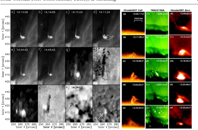
[image:6.595.79.409.71.246.2]Fig. 3 Left panel: evolution of a coronal jet observed inTRACE171 ˚A channel (a-f), SUMER (g-j) and MDI (k and l; the two arrows in this panel show the emerging magnetic flux). From Gontikakis et al. (2009). Right panel:evolution of a coronal jet observed by theHinodeSolar Optical Telescope (SOT) in Ca II (left column),TRACE195 ˚A (middle column) andHinode XRT (right column). From Nishizuka et al. (2008).
2.3STEREOObservations
The firstSTEREOobservations of jets were described by Patsourakos et al. (2008). This study provided clear evidence of helical structure in a polar coronal jet ob-served by EUVI onboard STEREO-A and -B (STA and STB, respectively; see Fig. 4). The helical structure was observed edge-on and face-on from the two re-spective viewpoints during the untwisting of the rising jet structure. This supplied solid evidence for a “true” helical structure something that was not possible to fully address with previous single-viewpoint observations. In addition, synthetic images from a 3D MHD jet model (Pariat et al., 2009) based on magnetic twist were found in qualitative agreement with the reportedSTEREOobservations (see right panels of Fig. 4).
Nistic`o et al. (2009) carried out a statistical survey of coronal jets (79 events) observed by SECCHI/EUVI and COR1 in both PCHs and ECHs. They found that about 40% (31/79) of the observed jets by EUVI had a helical structure. Therefore, a helical structure can be considered a common element of coronal jets. Moreover,
all reported jets of this study were associated with a compact magnetic bipole with the resulting jets observed either on top or at the side of these bipoles (“Eiffel tower” and “λ” jets, respectively; see Fig. 5). Note that SECCHI observations of jets suggest multipolar magnetic field settings (Filippov et al., 2013).
[image:7.595.71.416.73.299.2]et al., 2010, who termed them blow-out jets). Such blow-out jets often contain filament-like material in the erupting jet core as observed in the 304 ˚A channel. The association between blow-out jets and small CME-like eruptions was extended in a series of studies which combined STEREO with SDO, Hinode or PROBA2 observations. Typically one instrument provides a disk-view and the other a limb-view of the same event. Shen et al. (2012) found for a blow-out jet observed on disk by AIA which exhibited a bubble-like morphology when viewed off-limb by
STEREO. The bubble morphology is frequently observed in CMEs. Lee et al. (2013) analyzed EUVI observations showing an EUV dimming left behind by a jet observed off-disk withHinode. The association between twisted mini-filament eruptions and blow-out jets was also shown in Hong et al. (2011, 2013). All these findings suggest that the blow-out jets have significant similarities with the larger-scale CMEs and hint at a larger-scale-invariant eruptive solar phenomenon.
The width of EUV jets observed by EUVI ranges from down the instrument’s spatial resolution (i.e., 1.600≈1150 km) to few times 103−104km. By jet width we mean here the transverse spatial scale of the analyzed jet’s envelope and this does not incorporate any of the omni-present fine structure seen in jet observations.
STEREOobservations not only allowed to establish high correlations between EUV and WL jets (73−78% of 10,912 jets observed by COR1, Paraschiv et al., 2010) but also to provide insight into the kinematics and speeds of these events. Various methods were used for this task: triangulation (e.g., Patsourakos et al., 2008), image stack-plots (e.g., Pucci et al., 2013) and jet transit-times through the FOV of a given instrument (e.g., Nistic`o et al., 2009). The resulting jet speeds are in the range of ≈250−400 km s−1 and of ≈100−400 km s−1 for EUV and WL jets, respectively. From the statistical studies of Nistic`o et al. (2009) and Paraschiv et al. (2010) the average speeds of EUVI and COR1 jets are both around
≈300−400 km s−1. Note that most of the speeds quoted above correspond to the propagation phase of jets (i.e., after their initiation). Before reaching the typical cruising speeds of few hundred km s−1, the magnetic structure that eventually gives rise to a jet ascending at a much smaller speed of typically few 10 km s−1 (e.g., Patsourakos et al., 2008). This kinematic behavior (slow rise followed by impulsive acceleration) is a characteristic of an instability taking place in a quasi-statically driven MHD system (Pariat et al., 2009). PCH and ECH EUV jets have similar speeds as shown in Nistic`o et al. (2010).
Ratios of EUVI channel intensities have been used to estimate jet tempera-tures. Temperatures of 0.8−1.3 MK were found from 171/195 and 195/284 ratios (Nistic`o et al., 2011), while 284/195 and SXR ratios provided relatively higher temperatures of 1.6−2.0 MK (Pucci et al., 2013). This may in fact show that jets are not monolithic structures, but rather consist of different plasma components at different temperatures.
Fig. 4 (Left)STEREO ob-servations of a helical jet in a PCH (from left to right 195, 171 and 304 ˚A EUVI images). (Right) 171 ˚A im-ages of the jet compared with synthetic images from an MHD model. From Pat-sourakos et al. (2008).
Fig. 5 EUVISTEREO-A andSTEREO-B observations of an “Eifel Tower” (top) and of “λ”
jet (bottom). Both jets occurred within a PCH. From Nistic`o et al. (2009).
In a recent article, Nistic`o et al. (2015) studied the deflections of 79 PCH jets, at ≈1 and 2 R as observed by EUVI and COR1 respectively, and found that
their propagation was not radial and larger in the north than in the south. These properties were used to constrain models of the large-scale configuration of the coronal magnetic field.
2.4RHESSIObservations
[image:9.595.74.405.82.414.2]Fig. 6 (Left) RHESSI observations (colored contours) overlayed on co-temporal XRT observations (reverse color-table) of a coronal jet. From Chifor et al. (2008a). (Right)
RHESSI observations (col-ored contours) overlayed on co-temporal TRACE observations (reverse color-table) of a coronal jet. From Christe et al. (2008).
Two studies during coronal jets supplied evidence of HXR emissions not only from the bases of the observed jets but also from their spires (Bain & Fletcher, 2009; Glesener et al., 2012, see Fig. 7). Bain & Fletcher (2009) showed that the HXR emission corresponds to energies of 20-30 keV and the fitting of theRHESSI
spectrum provides evidence for a jet temperature of≈28 MK and the non-thermal nature of the emission, which was also corroborated by multi-frequency imaging observations in the microwaves by the Nobeyama radioheliograph. Off-limb obser-vations by Glesener et al. (2012) of a footpoint-occulted coronal jet showed faint HXR coronal sources along the jet spires reaching heights of≈50 Mm above the limb. The spectral analysis of the jet HXR source showed that collisional losses either in the corona or at the occulted chromospheric footpoints by accelerated electrons can supply the thermal and mechanical energy of the jet. Note that the-oretical calculations by Saint-Hilaire et al. (2009) placed limits on the number of non-thermal electrons accelerated along open magnetic field (e.g.,≈3×1036 for
RHESSI) to allow for their detection in HXRs or SXRs.
Frequently during coronal jets the temporal profile of the associated HXRs matches the associated type III radio burst. This suggests that the magnetic con-figuration associated with jets (i.e., transient magnetic field opening) released and accelerated electrons which escaped into the interplanetary space. The close tem-poral associations between coronal jets, HXRs, and type III radio bursts has been reported in a number of studies (e.g., Chifor et al., 2008a; Krucker et al., 2008; Berkebile-Stoiser et al., 2009; Bain & Fletcher, 2009; Glesener et al., 2012; Chen et al., 2013).
3Hinode/XRT and SDO/AIA Imaging: Morphology of Coronal Jets
Fig. 7 (Top) RHESSI observa-tions (colored contours) overlayed on co-temporal TRACE observa-tions (reverse color-table) of a coro-nal jet. From Bain & Fletcher (2009). (Bottom) RHESSI obser-vations (colored contours) overlayed on co-temporal TRACE observa-tions (reverse color-table) of a coro-nal jet. The red (blue) contours cor-respond to thermal (non-thermal) sources as determined from the corresponding spectral fittings dis-played at the bottom of this panel. From Glesener et al. (2012).
3.1 Standard and blow-out Jets
Based on these observations, they suggested that the narrow-spire jets were produced as in the original jet-production model due to Shibata (Shibata et al., 1992; Shibata, 2001, see§8); thus they dubbed these types of jets “standard jets,” since the jets seemed to obey that original “standard” picture (Fig. 8). In con-trast, they suggested that the broad-spire jets were generated by a variation of the standard picture. In this case, the emerging (or emerged) flux would have much more free magnetic energy than in the case where a standard jet was formed. They suggested that these jets started out the same as standard jets, with an emerging bipole reconnecting with ambient open field. That reconnection resulted in a narrow spire, as in the standard-jet case. But during this reconnection pro-cess, the emerging bipole is triggered unstable and erupts outward. This eruption blows out the bipole field and the surrounding field, carrying outward the cool (chromospheric-temperature) material entrained in those fields. Thus they named these types of jets “blow-out jets.” This eruption of the bipole results in much-more widespread reconnections than in the standard-jet case, where the emerging bipole remains inert throughout the jetting process. This scenario for blow-out jets could explain why the jet spire can grow from narrow to broad, and also why cool material, visible in 304 ˚A EUV images, would often accompany the blow-out jets (Fig. 8). An alternative possibility allowed for by Moore et al. (2010) is that the bipole starts erupting before the reconnection with the ambient field begins; in this view, the eruption of the bipole would drive the reconnection with the am-bient field. In both the standard and the blow-out cases, the suggestion was that the reconnection between the emerging or emerged bipole field and the ambient coronal field created the compact JBP. Fig. 9 shows the basic picture for standard and blow-out jets.
Moore et al. (2013) expanded upon the earlier work on standard and blow-out jets (Moore et al., 2010) by examining 54 X-ray jets found inHinode/XRT data, and they also observed them in AIA 304 ˚A images. They identified 32 of the jets as blow-out, 19 as standard, and 3 were ambiguous. When these newer results are combined with the previous work (Moore et al., 2010), the total number of X-ray jets examined is 109, and among these, 53 are standard, 50 are blow-out, and 6 are ambiguous. This new work (Moore et al., 2013) found that almost all blow-out jets (29 out of 32)1had corresponding jets observable in 304 ˚A images. They also found that almost none of the standard jets had such a cool jet visible in 304 ˚A; only 3 of the 19 standard jets had such a corresponding cool-component jet.
3.2 General Morphological Observations of Jets
In the last few years, analyses of coronal jets within CHs, QS, and in the vicinity of ARs based on multi-instrument observations (SDO/AIA and HMI, Hinode/XRT and EIS, and STEREO/EUVI) provided valuable insights into the morphology and causes of coronal jets. It has frequently been assumed or inferred that mag-netic reconnection is the cause of impulsive eruptions of jets following either flux emergence and/or cancellation. Different events showed different behavior and dy-namics.
1 A typo in paragraph 2 of§5 of Moore et al. (2013) says “all 29 blow-out X-ray jets displayed
(a) (b) (c) (d)
(e) (f) (g) (h)
(a) (b) (c) (d)
(e) (f) (g) (h)
Fig. 8 Examples of standard(Left)and blow-out(Right) jets observed byHinode/XRT.
Times are UT times on Sep. 22, 2008, and Sep. 20, 2008, respectively. The defining char-acteristics of standard jets are: narrow spire, compact JBP (c), and the absence of cool (chromospheric-temperature) emission inSTEREO/EUVI 304 ˚A images. Blow-out jets are, on the other hand, characterized by initially narrow spire (c) that later broadens to span nearly the width of the base region (e,f); initial compact brightening (b) that spread to the whole jet-base (c–e); and a strong cool (chromospheric-temperature) component visible in EUV 304 ˚A images. Adapted from Moore et al. (2010, see also Moore et al. 2013).
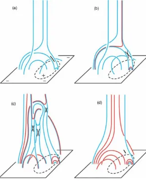
Fig. 9 Proposed process for blow-out jets,
according to Moore et al. (2010, 2013). (a) Initial set up is as in the case of stan-dard jets: ambient coronal magnetic field (open) and emerging or emerged bipolar field (closed). (b) Magnetic reconnection (X) occurs at the location of the current sheet (short black-line arch) shown in (a). A narrow jet spire resembling standard jets forms along the new open field lines. (c) Destabilization of the bipolar field lead-ing to full eruption and various reconnec-tions (crosses). Cool material originally en-trained inside of the bipole is carried out-ward with the eruption. (d) Late stages of the bipole’s eruption: new reconnection-produced loops form and brightening the base region of the jet. Adapted from Moore et al. (2010).
Regarding the morphological aspect of jets, studies of different events reported cases of fan-spine magnetic field topology following flux emergence (e.g., Liu et al., 2011a), evolution from standard to blowout type jet (Liu et al., 2011b), blowout resulting from mini-filament eruption (Hong et al., 2011; Shen et al., 2012; Adams et al., 2014, see Fig. 10), blobs and quasi-periodic small-scale plasma-ejection events along the jet spire (Zhang & Ji, 2014a; Chandrashekhar et al., 2014a,b), and hot and cold loops expanding out from a bright base forming a blowout jet (Young & Muglach, 2014a).
[image:13.595.75.417.71.210.2] [image:13.595.90.240.312.498.2]Fig. 10 On-disc observations of a blow-out jet, in (b1–b5) Hα from Big Bear Solar Observatory, (c1–c6) AIA 304 ˚A, and (d1– d6) AIA 193 ˚A. Panel (a) shows an HMI magnetogram, with a close up showing positive (p1) and negative polarities, and the contour of the of profile of the fil-ament labeled F1 in panel (b1). Vertical arrows show a bright patch prior to ejection of the fila-ment, and the two arrows in (d5) show the hot and cool compo-nents of the jet. From Shen et al. (2012).
also identified a faint, faster component (∼200 km s−1) in 193 ˚A images. The slow rise followed by a fast rise pattern is similar to that frequently observed in larger-scale filament eruptions (Roy & Tang, 1975; Sterling & Moore, 2005). It is also noteworthy that Hong et al. (2011) show that their jet had characteristics of large-scale CME-producing eruptions, including a small flare-like brightening, a small coronal dimming region, and a micro-CME. One is left to wonder whether solar activity is scale-invariant as noted by Raouafi et al. (2010).
Very recently Sterling et al. (2015) observed 20 near-limb PCH X-ray jets, using bothHinode/XRT andSDO/AIA images. They reported that all 20 jets originated from mini-filament eruptions, and with the JBP being flaring loops occurring in the wake of the eruption. Based on this, they suggested that the variety of coronal jet observed by Adams et al. (2014), rather than being exceptional, is in fact the
predominantvariety of coronal jet (at least in PCHs). They further suggested that standard jets and blow-out jets are fundamentally the same phenomenon, with either “standard” or “blow-out” morphology ensuing depending upon particulars of the mini-filament eruption. As of the time of this writing, it is too early to tell how well the Sterling et al. (2015) observations and inferences describe coronal jets in general.
The connection between CBPs and jets was discussed in studies by Hong et al. (2014) based onSDO/AIA and HMI. These CBPs are long-lasting features that are different from the transient jet base brightenings (i.e., the JBPs) that occur in conjunction with the jets themselves. From a study of 30 CBPs, they find that
∼25–33% of them experience one or more mini-filament eruptions, consistent with the blow-out-jet concept. They report that the mini-filament eruptions possibly result from flux convergence and cancellation.
HMI magentograms, did not find flux emergence in the jetting region, but sug-gested that emerging flux might be present but relatively weak. Shen et al. (2012) identified flux changes they interpreted as a series of flux emergences and cancel-lations that resulted in jet onset, and found indications of “impulsive cancellation between the opposite polarities during the ejection of the blow-out jet.” As far as we know, all other studies of the magnetic configuration (using HMI data) at the bases of observed jets reported flux cancellation as the cause of the jets (e.g., Hong et al., 2011; Adams et al., 2014; Young & Muglach, 2014a,b). So overall, we found that several observational studies provide evidence that flux cancellation leads to jets, while relatively few observational studies provide evidence that emerging flux leads to jets.
Zhang & Ji (2014a) suggest that the observed blobs are plasmoids ejected dur-ing reconnection resultdur-ing from teardur-ing-mode instability in current sheets occurrdur-ing with the jets.
We do not yet know with certainty the interrelationship between jets seen at different wavelengths. From Moore et al. (2010, 2013), we know that some X-ray jets have corresponding cooler-counterparts visible in AIA 304 ˚A, and other X-ray jets do not have such a cool counterpart. Apparently many if not all X-X-ray jets have EUV counterparts (e.g., Raouafi et al., 2008), but again a full study of the correspondence has not yet been undertaken. Therefore caution should be exercised to not generalize results from studies of jets seen at one wavelength to jets seen at substantially-different wavelengths. Thus for example, jets seen at, e.g., 171 ˚A and 211 ˚A should not be assumed to have counterparts at 304 ˚A or in X-rays; rather, data in those wavelengths should be checked before drawing conclusions.
4 Spectroscopic Observations of Jets
Spectrometers can observe the LOS bulk flow of plasma as if they were in-situ instruments and they can do this – in analogy to spectroscopic binaries – even for unresolved features. As such they ideally complement imaging instruments. In this Section we describe jet observations carried out by several spectrometers starting from the mid-90’s. These include observations bySOHO/CDS, SUMER, and UVCS,Hinode/EIS, andIRIS(see Table 3).
CDS consisted of two spectrometers (the normal incidence, NIS, and grazing incidence, GIS) fed by the same telescope that observed the 150–800 ˚A wavelength range. The NIS was far more widely used than the GIS, and so we focus only on results from the NIS. Two wavelength bands 308-381 ˚A and 515–632 ˚A were ob-served with a spatial resolution of 6–800, although following the temporary loss ofSOHO in 1998 the spatial resolution worsened to around 1000 and line profiles developed extended wings2. The wavebands consist mostly of emission lines from the upper transition region and corona (temperatures≥105 K), with the impor-tant exception of the strong Heiλ584.3 and Heiiλ303.8 emision lines (the latter
observed in the second spectral order).
In the SUMER spectral range from 660 ˚A to 1610 ˚A more than 1000 spectral lines are present that cover the vast temperature range from 0.005 MK (molecular
Table 3 Solar ultraviolet spectrometers.
Name Duration Wavelength Spatial Spectral Slits [˚A] Resolution Resolution
CDS 1996–2014 308–381, 6–1000 0.3-0.5 ˚A 200, 400 515–632a
SUMER 1996–2014 660-1610a 1.500 0.1 ˚A 0.300, 100, 400 UVCS 1996–2012 984–1080a, 2000 0.15-0.23 ˚A 3-10000
1100–1361
EIS 2006–present 170–212, 3–400 60 m˚A 100, 200 246–292
IRIS 2013–present 1332-1358, 0.33-0.400 26-53 m˚A 0.3300 1389-1407,
2783-2835 a2ndorder lines are also seen.
hydrogen) to 28 MK (Fexxiv), including the entire hydrogen Lyman series and a
significant part of the Lyman continuum. Centroiding techniques allow to detect Doppler flows down to 1–2 km s−1.
UVCS supplied detailed spectroscopic observations and diagnostics of jets in the outer corona from 1.4–10 R. The instrument observes in two wavelength
channels: the Ly-αchannel covering the range 1160–1350 ˚A and the Ovichannel covering the range 940–1123 ˚A (and 580–635 ˚A in the second order). The spec-trometer slit had a length of 40 arcmin. The main lines of the two channels were the Hi Ly-α line at 1215.7 ˚A, and the Ovi doublet at 1031.9 and 1037.6 ˚A. In
addition, UVCS observed lines including Hi Ly-β 1025.7 ˚A, Ciii 977.02 ˚A, Mgx
609.7 and 624.9 ˚A, Fexii1242 ˚A, and Sixii499.5 ˚A. These lines probe plasmas with temperatures in the range 0.03–2 MK. Given the weak signals from the outer corona, the analysis of UVCS observations frequently employs some binning along the slit leading to an effective spatial resolution≥2000. Finally, UVCS is equipped with a pinhole camera taking observations of the polarized radiance of the outer corona in the WL in the wavelength range 4500–6000 ˚A.
TheHinode/EIS observes the Sun observes the Sun in two narrow wavelength bands of 170–212 ˚A and 246–292 ˚A that are dominated by coronal emission lines from iron but also contain some cooler lines, in particular Heiiλ256.32 (Young et al., 2007). The key advance over CDS is the use of multilayer coatings on the optical surfaces that give enhanced sensitivity and enable higher quality imaging with a spatial resolution of 3–400.
4.1SOHO/CDS Results
A key discovery from CDS was the identification of twisting structures in macro-spicules, mostly observed in PCHs. Pike & Harrison (1997) presented the first event, which was observed just inside the solar limb at the south CH on 1996 April 11. The macrospicule was best seen in lines of Hei and Ov, but it had a
weak signature in Mgix(1 MK) and so we consider it to be a coronal jet. Although
Fig. 2 of this work shows Heiand Ovvelocity maps with a red- and a blue-shift on opposite sides of the jet, it was only highlighted in the later paper of Pike & Mason (1998) who found a similar signature in six other events. They coined the term “solar tornado” to describe this feature. Of further importance was the finding of an increasing velocity with height in the 1996 April 11 event, demonstrating that plasma continues to be accelerated along the body of the jet. Note that the velocity signatures from CDS only applied to the cool Hei and Ovlines as the signal was not strong enough in Mgixto derive accurate Doppler shifts.
The Pike & Harrison (1997) and Pike & Mason (1998) results were derived from individual rasters. A time sequence of the evolution of a hot macrospicule was presented by Banerjee et al. (2000), and this again showed weak Mgixemission, evidence for a twisted structure in Ov, and an increase in the Ovvelocity with
height.
4.2SOHO/SUMER Results
Wilhelm et al. (2002a) reported on the observation of a coronal jet on Mar. 8, 1999, in a single raster scan. The Neviii λ770.41 dopplergram showed a jet-like
structure extending to 35 Mm, with LOS speeds of∼40 km s−1.
A macrospicule at the limb of the south CH was reported by Popescu et al. (2007). It was observed on 1997 Feb. 25 with a sit-and-stare study, and showed a clear signature in Neviii λ770.41 and so we consider it to be a coronal jet. The
jet extended about 36 Mm above the limb and was present for 5 minutes. The jet emission was identified by a red-shifted component at 135 km s−1.
A unique observation was presented by Kamio et al. (2010) who observed an X-ray jet at the solar limb in a CH with Hinode/XRT. The STEREO/EUVI instruments observed a co-spatial macrospicule in the 304 ˚A filters, and SUMER and EIS rastered over the event, revealing hot emission in the Neviiiλ770.1 and Fexiiλ195.12 emission lines. The Doppler patterns in the cool lines observed by SUMER (Oiv λ790.20) and EIS (Heii λ256.32) suggested a rotating motion for
the broad macrospicule, and LOS speeds ranged from +50 to−120 km s−1. The coronal jet was visible in Neviiiλ770.40 as a very narrow streak extending above
the limb with a LOS speed of−25 km s−1.
Another example of a CH jet observed jointly by SUMER and EIS was pre-sented by Madjarska (2011), who observed a jet in an ECH on 2007 Nov. 14 using the SUMER sit-and-stare mode. The transition region lines (Ovλ629.70 and Nv
4.3SOHO/UVCS Results
Dobrzycka et al. (2000) presented the first detailed observations of coronal jets with UVCS. They analyzed a set of five polar jets, also tracked by EIT and LASCO, at radial distances 2.06-2.4 R. The passage of these polar jets through the UVCS slit
was manifested as increases in the intensity of the HiLy-α(30–75 %; see Fig. 11) and the Ovidoublet (50–150 %) lines. The increase took place either
simultane-ously in both HiLy-αand Ovior HiLy-αhad a delay of about 20 minutes with
respect to Ovi. Interestingly the observed spectral lines became narrower
dur-ing the observed jets, suggestdur-ing that the jets contained cooler plasmas than the background corona. Dobrzycka et al. (2000) applied two different models to one of the observed jets. The first model is a temperature-independent line-synthesis model and supplied estimates on plasma parameters. It was found out that during the jet passage through the UVCS slit the electron temperature decreased from
[image:18.595.120.367.375.478.2]≈0.75 MK to≈0.15 MK while the density decreased by a factor of≈1.2 from its initial value of 4.5×106cm−3. The outflow speed was estimated from the Doppler dimming effect to be > 280 km s−1; the observed jets exhibited small Doppler-shifts which suggests a quasi-radial flow. The second model was a time-dependent temperature and density non-ionization prescription of an expanding plasma par-cel which showed that an initial electron temperature<2.5 MK and heating rate commensurate to that of a ”standard” CH were required at the coronal base. This suggests that the heating requirements of coronal jets observed in CHs in the EUV and WL can be different and lower than those for the more energetic SXR jets.
Fig. 11 UVCS observations of jets.(Left)HiLy-αintensity a function of time and location
along the UVCS slit. The jet passage corresponds to the bright stripe seen around slit distance 40000(from Dobrzycka et al., 2000).(Right)Intensity images formed by stacking subsequent exposures at 1.64 Rin Ovi, HiLy-αand Ciiiat different times during a jet (from Ko et al., 2005).
In a follow-up study, Dobrzycka et al. (2002) analyzed UVCS observations of a set of 6 polar jets observed in HiLy-αand Ovibetween 1.5-2.5 R. This study
extended the basic results of the Dobrzycka et al. (2000) study. A heating flux of≈
3×10⁵erg cm−2s−1, based on the Wang (1994) plume model and non-equilibrium ionization calculations of a moving plasma parcel, at the coronal base was required to reproduce the jet emissions as observed by UVCS. The postulated heating flux had to be concentrated into a narrow region below 1.1 R and corresponded to
the observed jets and found densities comparable to plume values and 1.5 times higher than interplume densities at the same heights.
Ko et al. (2005) presented a comprehensive study of an AR coronal jet. The jet was traced from the Sun to the outer corona via an array of instruments including UVCS. The jet was associated with huge increases of several hundred with respect to the background corona in HiLy-αandβ, a factor 30 in Ciii, and
a factor 8 in Ovi (see Fig. 11). This suggests that the jet contained significant
amounts of cool material at around 105K. Significant Doppler-shifts first towards the blue (150 km s−1) and then towards the red (100 km s−1) were observed by UVCS; similar Doppler-shift evolution but this time first from the red and then to the blue was observed during the early stages of the jet at the limb by CDS and MLSO/CHIP (i.e., the Mauna Loa Solar Observatory/Chromospheric Helium-I Imaging Photometer). The UVCS Doppler-shift pattern correlated with the corresponding outflow velocities deduced via the Doppler-dimming effect. The changing signs of the jet’s Doppler-shifts both near the limb and in the outer corona may be consistent with rotation of the structure during its ascent.
Dobrzycka et al. (2003) analyzed five narrow CMEs (eruptions with angular width below 15◦) with the aim to study the possible connection between such eruptions and jets. The deduced plasma parameters of the narrow CMEs yielded similar speeds and somewhat higher densities and temperatures by a maximum factor of 2 compared to coronal jets. Taken altogether these findings did not suggest a clear dividing line between narrow CMEs and jets, which is consistent with the blow-out jets (Moore et al., 2010) which represent scaled-down versions of CMEs. Corti et al. (2007) analyzed observations of several cool jets during aSOHO -Ulysses quadrature. The jets were first observed by EIT in its 304 ˚A channel. Once they intercepted the UVCS slit at 1.7 Rstrong emissions in the cool lines Hi Ly-α and β, Ovi, and Ciii were recorded (e.g., > 10 times the background values
in in some lines). The jets were not observed in any of the hot lines available by UVCS. Empirical modeling of the spectral line intensities resulted in jet densities in the range (8.3−13)×106 cm−3 and temperatures of up to ≈ 1.7×10⁵ K. The jets’ average mass, gravitational, kinetic and thermal energies were estimated to 1013 g and 1.9×1028, 2.1×1027 and 1.5×1026 erg, respectively. Finally, no conclusive evidence for an in-situ detection of these jets by Ulysses was found.
4.4Hinode/EIS Results
We divide the EIS jets into CH and AR categories.
4.4.1 CH Jets
The key advance of the EIS spectrometer relevant to coronal jets (particularly in CHs) is the high instrument sensitivity for the Fexii λ195.12 emission line.
in sit-and-stare mode with the slit positioned about 11 Mm above the BP. The Fexiiline showed a two component structure, with a blue-shifted component at
240 km s−1. The second component was simply due to the CH background and was found at the rest wavelength of the line. This observation illustrates an important point when analyzing the Fexiiline: the corona is everywhere emitting at 1.5 MK,
and so the line profile of a jet is always a mixture of jet plasma and background plasma. In cases such as Moreno-Insertis et al. (2008) the two components are clearly separated, but the Kamio et al. (2007) jet is an example where the two are blended. By fitting only a single Gaussian to the Fexii line, the jet velocity is underestimated. A two Gaussian fit would have led to a larger velocity for the Kamio et al. (2007) jet component.
The CH jet studied by Kamio et al. (2010) (discussed in Sect. 4.2) was captured in a single EIS raster scan and observed as a very narrow streak in the Fexii
λ195.12 line, extending 75 Mm above the limb. The LOS velocity was−20 km s−1. Another jet observed simultaneously with SUMER was the ECH jet presented by Madjarska (2011) and discussed in Sect. 4.2. The jet was seen in a single raster scan, and the outflowing plasma was emitting in a wide range of lines from Heii
λ256.32 to Fexv λ284.16, and the LOS speed was up to 279 km s−1. A density
measurement in the jet was not possible, however.
Young & Muglach (2014a,b) and Young (2015) presented CH observations obtained from an EIS data-set that spanned almost two days during 2011 February 8–10 and captured a number of jets. Young & Muglach (2014b) studied a jet on the CH boundary for which the jet took the form of an expanding loop reaching heights of 30 Mm. The LOS speeds reached 250 km s−1, and evidence was found for twisting motions based on the variation of Doppler shift in the transverse direction of the jet. The density of the jet plasma, measured with a Fexiidensity diagnostic, was (0.9−1.7)×108 cm−3 and the temperature was 1.6 MK.
The largest and most dynamic jet from the data-set was presented by Young & Muglach (2014a). It extended to 87 Mm from the BP and LOS speeds reached 250 km s−1. The density of the jet plasma was 2.8×108cm−3and the temperature was 1.4 MK. A feature in common with the Young & Muglach (2014b) jet was the increase in LOS speed with height above the BP showing that plasma continued to be accelerated along the body of the jet. The jet BP showed a number of small, intense kernels as the jet began, reminiscent of flare kernels, and cool plasma was ejected as seen through an absorption feature in AIA 304 ˚A images.
Young (2015) demonstrated that almost half of the 24 jet events seen in the 2011 Feb. data-set showed no signature in AIA 193 ˚A image sequences, and so referred to them as “dark jets”. One dark jet was studied in detail, and was found to have a Fexiiλ195.12 intensity only 15–44% of the CH background. The LOS
speed of the jet plasma reached 107 km s−1 at a height of 30 Mm from the BP, and the temperature was 1.2–1.3 MK.
4.4.2 AR Jets
Chifor et al. (2008a,b) presented observations of a recurring jet on the west side of AR10938 during the period 15-16 Jan. 2007. One of the jets was captured in a single raster (Chifor et al., 2008b) in emission lines formed over the temperature range logT = 5.4 to 6.4. The signature of the jets was an extended short wavelength wing to the coronal emission lines with LOS speeds of 150 km s−1and very high densities (i.e., logNe≥11) as shown from diagnostics of Fexiiand Fexiiilines.
Other examples of AR jets were observed in AR10960 on Jun. 05, 2007 (Matsui et al., 2012) and at the limb in AR11082 on Jun. 27, 2010 (Lee et al., 2013). The ejected jet plasma in the Jun. 05, 2007 event could be identified in coronal lines up to logT = 6.4 (Fexviλ262.98). Taking into account the viewing geometries
of the twin STEREO spacecraft, accurate estimates of outward jet speed were inferred through analysis of lines formed over the temperature range logT = 4.9 to 6.4. The speed was found to increase with temperature in the corona from
≈ 160 to ≈ 430 km s−1, which is consistent with predictions for chromospheric evaporation during a reconnection process (Matsui et al., 2012). The Jun. 27, 2010 jet occurred on a large, closed loop and was very prominent in 304 ˚A images from AIA. EIS was running in sit-and-stare mode and the slit crossed through the jet about 40 Mm above the solar surface. A signal in Fexvλ284.16 is seen at the same time as X-ray emission is seen from XRT, confirming a jet temperature of around 2.2 MK. Evidence for twisting motions in the jet are found from simultaneous red and blue-shifts in Siviiλ275.36 (0.63 MK). For temperatures of 1–2 MK the jet
appeared as a dimming region that traveled along the loop. The density of the loop was estimated at 3×108 cm−3 from the Fexivλ264.79/λ274.20 ratio.
In summary, the AR jets observed by EIS are generally hotter than those seen in CHs, with the ejected plasma emitting in Fexvand Fexvi, suggesting
temper-atures of 2-3 MK. Further observations are needed to determine how common are jets with very high coronal density found by Chifor et al. (2008b).
4.5IRISResults
Cheung et al. (2015) reportedIRISobservations of recurrent coronal jets in an AR over a pore within a supergranule cell. The four observed homologous jets were observed in AIA coronal channels and the TR Siivlines at 1394 and 1403 ˚A. They
were characterized by relatively well-separated red- and blue-shifts of magnitudes of up to 50 km s−1across the jets’ axis. This line-shift pattern is consistent with helical motions. Tian et al. (2014) also reported IRIS observations of prevailing jet activity in the network at spatial scales of few hundred km.
5 Jet Dynamics: Statistics, CHs boundaries
5.1 Regionality of Coronal Jets
CHs (Savcheva et al., 2007). Although CH and QS jets are smaller than AR jets (Sako et al., 2013), averages of the apparent speeds are comparable and are about 200 km s−1. Plasma parameters such as temperature are characterized by larger error bars and are often model dependent. For details, see§4.
Subramanian et al. (2010) investigated transient brightenings, including jets, within CHs and quiet regions. They found that CH boundaries are particularly pro-lific in terms of brightenings occurrence and about 70% of these events within CHs and their boundaries show expanding loop structures and/or collimated outflows, while only 30% of the brightenings in QS show flows. Sako et al. (2013) analyzed over a thousand PCH (northern) and QS jets. They found that jet occurrence rate in CH boundaries is twice as large as that in PCHs. Flux emergence/cancellation rates cannot explain this difference (Sako et al., 2013). Yang et al. (2011) re-ported on westward shifts in the boundaries of CHs so that their rigid rotation is maintained. It can be easily imagined that a coronal jet is produced by magnetic reconnection between the open field in a CH and the closed loop in a quiet region (i.e., interchange reconnection), which suggest that the coronal (global) magnetic topology need to be considered for understanding this phenomenon.
5.2 Dynamics of Coronal Jets
Except for the rare occurrence of large jets (Shibata et al., 1994),Yohkoh/SXT observations did not allow investigating the inner structure and evolution of jets. Alexander & Fletcher (1999) used Yohkoh-TRACE joint observations to obtain some insight into jets’ fine structure. The recent high-quality X-ray/EUV data fromHinode, STEREO, and SDOreveal the complex structure and dynamics of these coronal events. In the following sections, we discuss the dynamics of coronal jets from the morphology and statistics point of view.
5.2.1 Transverse Motion
Shibata et al. (1992) reported on a coronal jet moving sideways with velocity of 20– 30 km s−1. Canfield et al. (1996) used jet reconnection model to interpret whip-like motions and footpoint blue-shifts of coronal jet-associated H-αsurges. Neverthe-less, detailed observations of jet transverse motions were uncovered using on-disk and mainly off-limb Hinode observations. A statistical study by Savcheva et al. (2007) of 104 PCH events showed that more than 50% of jets display transverse motions with∼35 km s−1. Chandrashekhar et al. (2014a) found that the transverse motion speed decreases with increasing height. Higher velocity (> 100 km s−1) transverse motions have been reported by Shimojo et al. (2007) in several coro-nal jets, and that one event showed whip-like motion presumably following the opening of reconnected closed field lines. It can be easily speculated that whip-like motions result from the relaxation of the reconnected guide magnetic field.
There are two flavors of jet transverse motions: expanding motions and os-cillations. Moore et al. (2010) interpreted expanding jets as “curtain-like spires”. Theoretically, the speed of the reconnected flux is 100−1000 km s−1 assuming an Alfv´en speed of 1000 km s−1 (Canfield et al., 1996). The observed speeds (i.e.,
This may hint at expansion of the reconnection region rather than motion of re-connected magnetic flux. On the other hand, Cirtain et al. (2007) reported the first detection of the transverse oscillations in a coronal jet, which can be used to infer a number of physical parameters (e.g., temperature, magnetic field) in the corona using magneto-seismology. Morton et al. (2012) studied oscillations of a jet dark thread (i.e., the jet’s inner structure) and found a period of 360 seconds. They in-ferred a temperature of<3×10⁴K from kink mode oscillations. Chandrashekhar et al. (2014b) analyzed oscillations of the bright thread of a CH-boundary jet. They inverted the oscillation’s 220 second period into magnetic field strength of 1.2 Gauss. They also reported strong damping of the transverse oscillations that are characterized by a velocity amplitude of 20 km s−1.
In view of the recent results by Sterling et al. (2015), which suggest that coronal jets may be the result of eruption of small-scale filaments (see §3.2), a distinguishing characteristic of the emerging-flux and the minifilament ideas is the expected drift with time of the jet spire with respect to the JBP location. Sterling et al. (2015) predict that the spire should tend to driftawayfrom the BP, while the emerging-flux model should result in the spire driftingtoward the BP. Savcheva et al. (2009) find that the drift is often away from the JBP (supporting the Sterling et al. 2015 interpretation), although this question should be investigated more systematically.
5.2.2 Untwisting Motions of Jet Helical Structure
Patsourakos et al. (2008) successfully reconstructed a coronal jet in 3D using near-simultaneous observations from the STEREO twin spacecraft. They unam-biguously showed the helical structure of the jet, which was later confirmed through 3D-MHD simulations by Pariat et al. (2009). The morphological analysis of Nis-tic`o et al. (2009) described in Sect. 2.3 confirm that helical jets are common and that untwisting motions may also be an important property of a significant class of jets.
Similar to the earlier-mentioned Shen et al. (2012) paper, several other works have discussed winding or twisting motions of EUV jets observed in AIA data (see Fig. 12). In this Section we highlight several of these papers, although some papers noted elsewhere also discuss twists in jets. Such twists could be important with regards to the driving of jets, and perhaps may even be important for the energization and mass balance of the upper atmosphere.
Various studies reported twisting motions in coronal jets occurring in different regions (i.e., CHs, QS, ARs). While it has not been rigorously established that coronal jets in ARs are the same as those occurring in CH regions, the natural expectation is that most coronal jets would share similar or identical driving pro-cesses. Jets with<∼1
4−2.5 turns have been observed. Specifically, Shen et al. (2011)
showed a near-limb polar jet unwinding as it erupted, showing ∼1−2.5 turns. Moore et al. (2013) analyzed a large sample of 32 jets and found different degrees of jet twisting in 29 of their events: ten of these had modest twists of<∼ 14 turns, 14 had twists of between 1
4 and 1
2 turns, while 5 jets had turns ranging from 1 2 to 5
2 turns (Fig. 13).
Fig. 12 AIA 171 ˚A images of undulating jet, from 2010 September 17. Panel (a) shows six different heights for which distance-time plots are shown in (b). In (b), the dashed black line highlights the undulating pat-tern, and the white lines show features tracked though the dif-ferent panels at the indicated ve-locities. From Schmieder et al. (2013).
Fig. 13 Histogram showing amount of
twist observed in AIA 304 ˚A movies of X-ray coronal jets, giving the number of jets and the amount of rotation (twisting or unwinding) during the observed lifetime of the 304 ˚A jets. From Moore et al. (2013).
images, with plane-of-sky velocities of∼30–60 km s−1, that were decreasing with increasing height. Spectroscopic observations fromHinode/EIS show Doppler ve-locities blueshift- and redshift-veve-locities of∼70 km s−1and 8 km s−1, respectively, and the authors point out that these shifts could be due to the helical motions. Zhang & Ji (2014b) also found twisting motions within a jet/surge event with an average∼120 km s−1 that subsequently slowed down to∼80 km s−1. An AR jet observed by Liu et al. (2014) showed twisting motions with velocities in the range 30−110 km s−1. Other works (e.g., Chen et al., 2012; Hong et al., 2013) also provide quantitative values for twisting motions in AIA-observed jets.
[image:24.595.80.428.65.498.2]jets. The distinctive signature of these motions in Dopplergrams is positive and negative LOS-velocities side-by-side along the flow direction, which is a common feature in cool jets (i.e., H-αSurge: ¨Ohman et al. 1968, Xu et al. 1984, Gu et al. 1994, Canfield et al. 1996; spray: Kurokawa et al. 1987; macrospicule: Pike & Ma-son 1998, Kamio et al. 2010; AR jet: Curdt et al. 2012). EUV observations, on the other hand, seems to point that untwisting motions may not be a common property of EUV jets (Kamio et al., 2007; Matsui et al., 2012). This inconsistency between stereoscopic and spectroscopic observations maybe due to the fact that spectrometers can detect subresolution flows.
One other possibility is that the sensitivity, spatial resolution and time cadence of current spectroscopic observations may not be sufficient for the measurement of untwisting motions. If this is correct, untwisting motions should be significantly slower than the flow. To understand the driving mechanism of coronal jets, es-pecially to evaluate the contribution ofJ×Bforce for accelerating a coronal jet (Shibata & Uchida, 1986), it is essential to know the properties of untwisting mo-tion. New instruments with better capabilities are also needed. RecentIRIS spec-troscopic observations with their superior spatial and temporal resolution show ubiquitous untwisting motions at chromospheric level (de Pontieu et al., 2014b), and twisting motions in AR jets at transition region temperatures have been re-ported by Cheung et al. (2015). However,IRISmay not be able to detect coronal signatures of twisting as the only available coronal line (Fexii1349 ˚A) is too weak.
In addition to twisting motions, periodic dynamics, ranging from∼50 s (Mor-ton et al., 2012) to∼20 min (Liu et al., 2014; Zhang & Ji, 2014b), have been also found in connection with these motions.
5.2.3 Apparent Speed of Coronal Jets
Since the flow speed is a key parameter for understanding the acceleration mech-anism(s) of jets, different approaches have been adopted for the measurement of apparent speeds. Since polar jets are nearly-radial, the difference between the ap-parent and real speeds may be small. For AR jets, additional information, such as spectroscopic measurements, is needed. Matsui et al. (2012) and Sako (2014) measured speed for relatively long jets (< few ×104 km) using STEREO data. They found that apparent speeds are 10−20% smaller than real velocities. This indicated that using apparent speeds might be adequate in most cases keeping in mind that these velocities are the lower limits.
0 200 400 600 800 1000 Speed [km s-1]
5.5 6.0 6.5 7.0 7.5 8.0
Log
10
Temperature [K]
2 [G] 5 [G]
10 [G]
25 [G]
50 [G] 100 [G]
200 [G]
[image:26.595.105.379.76.257.2]500 [G]
Fig. 14 Temperature-speed map for thermally- (evaporation) and magnetically-driven jets.
The regions between the thin and solid curves correspond to the temperature-speed domains where magnetically- and thermally-driven jets occur, respectively. The intersection between the two regions indicates where both jet classes coexist. The red, green and blue symbols correspond to jets occurred in ARs, QS, and CHs, respectively. The colored solid/dashed lines indicate theoretical predictions of the magnetic field strength. From Sako (2014).
component is magnetically driven. Sako (2014) studied a number of long jets and classified them into thermal or magnetic dominated events based on comparison of the observed temperature – speed relation with theoretical predictions (Fig. 14). He found that both classes exist all over the solar disk and that in ARs the number of thermally-driven jets is larger than the magnetically-driven ones. In CHs and QS, however, jets are distributed in the overlapping region of the temperature-speed map (Fig. 14). From their result, it is not clear what physical parameter is most important for the selection of the jet dominant component. The magnetic field strength is an important parameter but not critical since both jet classes oc-cur in all regions. Magnetic topology and free energy may be necessary to address this question.
6 Relationship to other coronal structures
6.1 Jet – Plume Connection
Coronal jets are characterized by their transient nature and often appear as col-limated beams presumably guided by open magnetic fields. In contrast, coronal plumes, which are most prominent and pervasive within CHs, are hazy without sharp edges as seen in EUV 171 ˚A and WL images. They are also significantly wider than jets (∼20−40 Mm; Wilhelm, 2006) , may reach up to∼30Rabove
the solar surface (Deforest et al., 1997), and are quasi-stationary during their life-time spanning in the order of days. Prior to theSTEREO/Hinodeera, coronal jets and plumes have been studied independently and any eventual interrelationship has not been considered. They, however, share common characteristics. They are both episodic in nature and are usually rooted in the chromospheric network where magnetic reconnection is thought to play a key role in their formation (Canfield et al., 1996; Wang, 1998). The connection between jets and plumes is important for understanding their formation processes and evolution and their eventual con-tribution to the heating and acceleration of the SW.
Fig. 15 EUV 171 ˚A
im-ages from SECCHI/EUVI on STEREO-A illustrating the connection between coronal jets and plumes. Jets are of-ten observed to erupt prior to and during the lifetime of plumes. Top panels: erup-tion of a CBP into a jet (white arrows). Bottom-left: disappearance of the coronal jet. Bottom-right: appearance of plume haze (white arrow). A time lag ranging from minutes to several tens of minutes is typically observed between the jet disappearance and plume formation. From Raouafi et al. (2008).
Raouafi et al. (2008) investigated the jet-plume relationship usingHinode/XRT andSTEREO EUV observations that were recorded during the deep solar mini-mum (2007 Apr. 7-8; see Fig. 15). A total of 28 X-ray jets were analyzed. Raouafi et al. (2008) discovered that>90% of the jets were associated with plume haze and
1997). Their interpretation of the observations is that jets result from impulsive magnetic reconnection of emerging flux (e.g., Yokoyama & Shibata, 1995), where plumes may be the result of lower-rate magnetic reconnection as shown by the short-lived, small-scale BPs and jet-like events observed within their footpoints.
More recent findings (e.g., Kamio et al., 2010; Wilhelm et al., 2011) provide evidence that polar jets occur in the interplumeregion next to a plume and that the jet plasma probably feeds the plume. SUMER observations (Wilhelm et al., 2002b) revealed an increased line width in plumes, but no net flow in plumes. Dwivedi & Wilhelm (2015) presented a model assuming a plume as quasi-closed volume, where plasma of the polar jet is trapped and continuously moves up and down, thus operating the strong FIP effect.
Recently, Raouafi & Stenborg (2014) took advantage of the high-quality data from the SDO/AIA and HMI to analyze the coronal conditions leading to the formation and evolution of coronal plumes. Prior to theSDOera, the spatial and temporal resolution of the imaging instruments were limited and therefore coronal plumes and their fine structure could not be fully resolved and their temporal evolution could not be analyzed in detail. This might be the reason that coronal plumes are often referred to in the literature as “hazy” structures and heuristic assumptions on the plasma heating and acceleration at their source regions are typically the norm in numerical models.
Raouafi & Stenborg (2014) focused particularly on the fine structure within plume footpoints and on the role of transient magnetic activity in sustaining these structures for relatively lengthy periods of time (several days). In addition to nom-inal jets occurring prior to and during the development of plumes, the data show that a large number of small jets (“jetlets”) and plume transient BPs (PTBPs) occur on timescales of tens of seconds to a few minutes. These features are the result of quasi-random cancellations of fragmented and diffuse minority magnetic polarity with the dominant unipolar magnetic field concentration over an extended period of time. They unambiguously reflect a highly dynamical evolution at the footpoints and are seemingly the main energy source for plumes. This suggests a tendency for plumes to be dependent on the occurrence of transients (i.e., jetlets, and PTBPs) resulting from low-rate magnetic reconnection. The present findings may be of great importance for the interpretation of future measurements by dif-ferent instruments on board the Solar Probe Plus and Solar Orbiter. These future measurements may provide further details on the plasma thermodynamics, such as heating and acceleration of SW particles within coronal plumes.
6.2 Jet-Sigmoid Connection
Raouafi et al. (2010) used observations from XRT, EIS, and EUVI to study the morphology and fine structure of XBPs leading to coronal jets in conjunction with their characteristics (i.e., untwisting motions, transverse apparent motions, etc.). The resolved structure of some BPs is more complex than previously assumed. Several jet events in the CHs are found to erupt from small-scale, S-shaped bright regions (see Fig. 16). This finding suggests that coronal small-scale (micro-) sig-moids (Rust & Kumar, 1996) may well be progenitors of coronal jets. Moreover, the presence of these structures may explain numerous observed characteristics of jets such as helical structures, apparent transverse motions, and shapes.
Fig. 16 Hinode/XRT
obser-vations of XBPs evolving into micro-sigmoid and then erupt-ing into jets. For details see Raouafi et al. (2010).
Patsourakos & Raouafi (2016, in preparation) investigated the case of a small sigmoidal BP within an ECH. The underlying magnetic fields show significant emergence as well as cancellation that lead to the formation of the sigmoid, which lasted for several hours. The full eruption of this sigmoid was the result of the cancellation of large magnetic flux that resulted in a large jet. This analysis shows that the evolution of the small-scale coronal features have similarities with large magnetic regions.
7 Jets, Solar Wind, and Solar Energetic Particles
7.1 Association Between Jets and Impulsive Solar Energetic Particle Events
radio bursts (see Kahler et al., 1987). They are particularly found to coincide also with X-ray jets (Kundu et al., 1995; Raulin et al., 1996; Glesener et al., 2012). A review by Reames (1999) provides details on the characteristics of these two classes of SEP events.
Historically, the lack of understanding of the origin of impulsive SEP events may be due to the lack of high-resolution, both temporal and spatial, solar ob-servations that are necessary for the identification of small-scale activity. SEPs during the latest solar maximum were observed with unprecedented precision and breadth by a new generation of instruments on ACE, Wind, SAMPEX, SOHO,
[image:30.595.87.402.225.340.2]TRACE,Hinode, andRHESSI.
Fig. 17 Evolution of a coronal jet coinciding with a type III burst and an electron event.
(a) Radio dynamic spectra and X-ray light curve. (b) The electron flux at 1 AU. (c) XRT negative intensity image of the jet source region. (d-h) Running-difference images illustrating the evolution of the flare and the jet. From Nitta et al. (2008).
Wang et al. (2006) investigated the solar sources of 253He-rich events through the analysis of EUV and WL coronagraph observations from SOHO/EIT and LASCO, respectively. They also used a potential field source surface (PFSS) mag-netic field model to determine the magmag-netic connectivity of Earth to the solar surface, as well as Hei10830 ˚A images to locate CHs. They suggested that3
He-rich events originated from coronal jets erupting at the interface between ARs and adjacent open field regions.
Nitta et al. (2006) studied 117 impulsive SEP events between Dec. 1994 and Dec. 2002. They used particle measurements from the WIND/EPACT/LEMT (von Rosenvinge et al., 1995), solar EUV and X-ray images fromSOHO/EIT and