A
NALYSIS
& PDE
msp
Volume 11
No. 1
2018
J
ONATHANM. F
RASER ANDT
UOMASS
AHLSTENVol. 11, No. 1, 2018
dx.doi.org/10.2140/apde.2018.11.115
msp
ON THE FOURIER ANALYTIC STRUCTURE OF THE BROWNIAN GRAPH
JONATHANM. FRASER AND TUOMASSAHLSTEN
In a previous article(Int. Math. Res. Not.2014:10 (2014), 2730–2745)T. Orponen and the authors proved that the Fourier dimension of the graph of any real-valued function onRis bounded above by 1. This partially answered a question of Kahane (1993) by showing that the graph of the Wiener processWt
(Brownian motion) is almost surely not a Salem set. In this article we complement this result by showing that the Fourier dimension of the graph ofWt is almost surely 1. In the proof we introduce a method
based on Itô calculus to estimate Fourier transforms by reformulating the question in the language of Itô drift-diffusion processes and combine it with the classical work of Kahane on Brownian images.
1. Introduction and results
1A. Geometric properties of Brownian motion. Gaussian processes are standard models in modern probability theory and perhaps the most well-studied example is theWiener process(or standardBrownian motion)W =Wt :R>0→Rcharacterised by the propertiesW0=0, the mapt7→Wt is almost surely continuous, andWt has independent increments such thatWt−Wsfort>s is normally distributed:
Wt−Ws∼N(0,t−s).
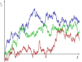
The Wiener process has far-reaching importance throughout mathematics and it is a topic of particular interest to understand its geometric structure. This can be achieved by studying several random fractals associated to the process such asimages W(K):= {Wt:t∈K}of compact setsK ⊂ [0,∞),level sets Lc(W):= {t∈R:Wt =c}for c∈R,graphs G(W):= {(t,Wt):t∈R}(seeFigure 1) and other more delicate constructions such as SLEκ-curves.
The basic properties of Brownian motion mean that these random fractals enjoy a certain “statistical self-similarity”, which facilitates computation of their Hausdorff dimensions dimH. Classical results include McKean’s proof[1955]that dimHW(K)=min{1,2 dimHK}almost surely for each compact K ⊂ [0,∞). Moreover, for the level sets, dimHLc(W)=12 almost surely forc=0 by[Taylor 1955]and for allc∈Rby[Perkins 1981]conditioned on Lc(W)being nonempty. For the Brownian graphG(W), Taylor[1953]proved that dimHG(W)= 32 almost surely and Beffara[2008]computed the Hausdorff dimensions of SLEκ-curves. Moreover, Hausdorff dimensions for similar sets given by many other Gaussian processes, such as fractional Brownian motion, have been also considered; see, for example,
Fraser acknowledges financial support from the Leverhulme Trust (RF-2016-500) and Sahlsten acknowledges the support from the European Union (ERC grant no. 306494 and Marie Skłodowska-Curie Individual Fellowship grant no. 655310).
MSC2010: primary 42B10, 60H30; secondary 11K16, 60J65, 28A80.
Keywords: Brownian motion, Wiener process, Itô calculus, Itô drift-diffusion process, Fourier transform, Fourier dimension, Salem set, graph.
Wt
[image:3.500.165.335.74.202.2]t
Figure 1. Three realisations of the graphG(W)for the Brownian motionWt.
Adler’s classical results[1977]for fractional Brownian graphs and the recent work[Peres and Sousi 2016]concerning variable drift.
1B. Fourier analytic properties of Brownian motion. The Hausdorff dimension is the most commonly used tool for measuring the size of a set Abut there is also another fundamental notion based on Fourier analysis which reveals more arithmetic and geometric features of A, including curvature, which are not seen by the Hausdorff dimension. This is based on studying the Fourier coefficientsof a probability measureµon A⊂Rd, which are defined by
ˆ
µ(ξ):=
Z
e−2πiξ·xdµ(x), ξ∈Rd.
Now the size of Acan be linked to the existence of probability measuresµon Awith decay of Fourier coefficientsµ(ξ)ˆ when|ξ| → ∞. The following connection between Hausdorff dimension and decay of Fourier coefficients is well known and goes back to Salem and Kaufman, but we refer the reader to[Mattila 2015]for the details. If dimHA>s, then Asupports a probability measureµwith| ˆµ(ξ)| =O(|ξ|−s/2) “on average”, that is,RRd| ˆµ(ξ)|2|ξ|s
−ddξ <∞, and vice versa the Hausdorff dimension can be bounded from below if such a measure µ can be found. It is possible, however, that dimHA=s >0 but no measureµon Ahas Fourier decay at infinity; this happens for example when Ais the middle-third Cantor set inR. Therefore, one defines the notion ofFourier dimensiondimFAof a set A⊂Rd as the supremum ofs∈ [0,d]for which there exists a probability measureµsupported on Asuch that
| ˆµ(ξ)| =O(|ξ|−s/2) as|ξ| → ∞. (1-1)
Finding measuresµon Awith polynomially decaying Fourier transform (i.e.,(1-1)for somes>0) has deep links to absolute continuity, arithmetic and geometric structure, and curvature. If Asupports a measureµsuch that(1-1)holds withs>1, then Parseval’s identity yields thatµis absolutely continuous to Lebesgue measure and Amust contain an interval. An application of Weyl’s criterion known as the Davenport–Erd˝os–LeVeque criterion[Davenport et al. 1963] yields that inR polynomial decay ofµˆ guarantees that µalmost every number is normal in every base and an interesting result of Łaba and Pramanik[2009]shows that if thesin(1-1)is sufficiently close to 1 for a Frostman measureµon A⊂R and there is a suitable control over the constants, see the recent work[Shmerkin 2017], thenAcontains nontrivial 3-term arithmetic progressions. Moreover, an analogous result also holds for higher dimensions with arithmetic patches[Chan et al. 2016].
On the curvature side, if Ais a line-segment inR2, then Acannot contain any measure with Fourier decay at infinity so A cannot be a Salem set. However, if A is an arc of a circle or more generally a 1-dimensional smooth manifold with nonvanishing curvature then the 1-dimensional Hausdorff measureµ on A satisfies(1-1)withs=1; see[Mattila 2015]. In particular, Ais a Salem set. In these examples of Aone can observe that the important arithmetic or curvature features present are not seen from the Hausdorff dimension.
Constructing explicit Salem sets (which are not manifolds), or just sets Asupporting a measureµ satisfying(1-1)for somes>0, can be achieved through, for example, Diophantine approximation by [Kaufman 1980;1981;Bluhm 1998;Queffélec and Ramaré 2003] or via thermodynamical tools by[Jordan and Sahlsten 2016]. However, for random sets it has been observed in many instances thatAis either almost surely Salem or at least supports a measureµwith(1-1)for somes>0. This was first done for random Cantor sets by Salem[1951], where Salem sets were also introduced. Later in his classical papers, Kahane [1966a;1966b]found out that the Wiener process and other Gaussian processes provide natural examples.
Since Kahane and Salem, the study of Fourier analytic properties of natural sets derived from Gaussian processes and more general random fields has been an active topic. For the Brownian images, Kahane [1985b]proved that for any compactK ⊂Rthe imageW(K)is almost surely a Salem set of Hausdorff dimension min{1,2 dimK}. Kahane also established a similar result for fractional Brownian motion. Łaba and Pramanik[2009]then applied these to the additive structure of Brownian images. Later Shieh and Xiao[2006]extended Kahane’s work to very general classes of Gaussian random fields. However, understanding the Fourier analytic properties of the level sets and graphs remained an important problem for some time. Kahane[1993]outlined the problem explicitly.
Problem 1.1(Kahane). Are the graph and level sets of a stochastic process,such as fractional Brownian motion,Salem sets?
almost surelynota Salem set[Fraser et al. 2014]. It turned out that the reason for this is purely geometric: the proof was based on the following application of a Fourier-analytic version of Marstrand’s slicing lemma.
Theorem 1.2[Fraser et al. 2014, Theorem 1.2]. For any function f : [0,1] →Rthe Fourier dimension of the graph G(f)cannot exceed1.
Indeed, since dimHG(W)= 32 >1 almost surely[Taylor 1953], this answers Kahane’s problem in the negative for the Wiener process. Note that this also gives a negative answer for fractional Brownian motion since the Hausdorff dimension in that case is also strictly larger than 1 almost surely.
The methods in [Fraser et al. 2014] are purely geometric and involve no stochastic properties of Brownian motion. They also do not shed any light on the precise value for the Fourier dimension ofG(W). Note that even though dimHG(f)>1 for any continuous f : [0,1] →R, the Fourier dimension of a graph may take any value in the interval[0,1]; see[loc. cit.]. For example, dimFG(f)=0 if f is affine and, moreover, dimFG(f)=0 for theBaire generic f ∈C[0,1]; see [loc. cit., Theorem 1.3].
The main result of this paper is to complete the work initiated by Kahane’s problem in the case of Brownian motion by establishing the precise almost sure value of the Fourier dimension ofG(W).
Theorem 1.3. The graph G(W)has Fourier dimension1almost surely.
Moreover, the random measureµwe use to realise the Fourier dimension is Lebesgue measuredton [0,1]lifted onto the graphG(W)via the mappingt7→(t,Wt). The precise estimate we obtain is that almost surely
| ˆµ(ξ)| =O(|ξ|−1/2plog|ξ|) as|ξ| → ∞, (1-2)
which combined withTheorem 1.2yieldsTheorem 1.3.
A natural direction in which to continue this line of research would be to study other Gaussian processes with different covariance structure, such as the fractional Brownian motion.
1C. Methods: Itô calculus and reduction to Brownian images. The key method we introduce to esti-mate the Fourier transform of the graph measureµis based onItô calculus, which has previously been a natural framework in the theory of stochastic differential equations. As far as we know, Itô calculus has not been previously considered in this Fourier analytic context. Here we discuss this method and give a brief summary of the main steps in the proof. When written in polar coordinates,(1-2)asks about the rate of decay for the integral
ˆ
µ(ξ)=
Z 1
0
exp(−2πi u(tcosθ+Wtsinθ))dt
forξ=u(cosθ,sinθ)∈R2, u>0, θ∈ [0,2π), asu→ ∞. There are two distinct cases we will consider depending on the direction ofξ, which we give a heuristic description of here.
orπ, we still have a small random (nonsmooth) termWtsinθ, so a classical change of variable formula or other tools from classical analysis cannot be used.
The key observation is that we can writeµ(ξ)ˆ =R exp(i Xt)dt, where the stochastic processXt satisfies the stochastic differential equation
d Xt :=b dt+σd Wt,
identifying it as a so-calledItô drift-diffusion process, whereb:= −2πucosθ is the drift coefficient of Xt andσ:= −2πusinθ is thediffusion coefficientofXt. Such processes have many useful analytic tools from Itô calculus (seeSection 2) associated to them, in particularItô’s lemma, which works as an analogue for the chain rule. The price we pay is that Itô’s lemma introduces some multiplicative error terms involving stochastic integrals, but they can be estimated with other tools from Itô calculus using moment analysis.
The estimates we obtain from Itô calculus allow us to obtain the correct Fourier decay(1-2)forµ whenθ is close to 0 orπ with respect tou−1 (more precisely,|sinθ|<u−1/2), in other words, whenξ is close to pointing in the horizontal directions. Thus another estimate is needed for θ bounded away from 0 andπ. This is where the classical work[Kahane 1985b]on Brownian images comes into play. If we completely ignore the deterministic componenttcosθ, by settingθ= π
2 or 3π
2 , thenµ(ξ)ˆ is the Fourier transform of the Brownian image measureν, that is, thet7→Wt push-forward of the Lebesgue measuredt on[0,1]atu. Kahane[1985b]in fact already established that the decay of| ˆν(u)|is almost surely of the orderu−1plogu= |ξ|−1plog|ξ|so(1-2) holds for these directions. A modification of Kahane’s argument reveals that wheneverθ 6=0 orπ, then almost surely
| ˆµ(ξ)| =O(|sinθ|−1|ξ|−1plog|ξ|);
see the discussion inSection 3C. Now one notices that whenθ approaches 0 orπ, this estimate blows up, and so one cannot obtain a uniform estimate over all directions from this. However, this gives(1-2) if|sinθ|>u−1/2, so combining with the estimates we obtained through Itô calculus, we are done. See Section 3for more details on the main steps of the proof.
1D. Other measures on the Brownian graph. Theorem 1.3and(1-2)give Fourier decay for the push-forward of the Lebesgue measure on[0,1]onto the graphG(W). It would be an interesting problem to see if one can have similar results for other, possibly fractal, measures on[0,1]. A possible problem could be:
Problem 1.4. Classify measuresτ on[0,1]such that for some0<s61we have
| ˆτ(ξ)| =O(|ξ|−s/2), |ξ| → ∞,
and their liftµτ onto the graph of G(W)under t7→(t,Wt)satisfies
| ˆµτ(ξ)| =O(|ξ|−s0/2), |ξ| → ∞ for any s0<s.
andπ we could still boundµˆτ(ξ)using Kahane’s work. The main problem in generalising our approach to fractal measuresτ on[0,1]comes from the lack of an appropriate analogue of It¯o calculus.
1E. Organisation of the paper. InSection 2we give the necessary background from Itô calculus. In Section 3we will give the proof of our main result Theorem 1.3. The key estimates are obtained in Section 3BandSection 3C, corresponding to the two cases discussed above.
2. It¯o calculus
2A. Stochastic integration. In the proof of the main resultTheorem 1.3, we end up studying integrals of the formR f(Xt)dt for some stochastic processes Xt and smooth scalar functions f. As standard analysis methods cannot be applied to these integrals, we need theory from stochastic analysis. Stochastic analysis provides a pleasant framework to deal with nonsmooth processes, such as the Wiener processWt, and still preserves many of the classical features present in the smooth setting. In this section we discuss the specific tools fromItô calculuswhich we will rely on. The main references for this section are given in the book[Karatzas and Shreve 1991].
Let(,F, (Ft)t>0,P)be a filtered probability space; that is,Ft⊂Fis an increasing filtration int. Let W=Wt be the Wiener process adapted to this filtered probability space; that is,Wt isFt measurable and for eacht,s>0 the incrementWt+s−Wt is independent ofFt. We say that anR- orC-valued stochastic process Zt isadaptedif it isFt measurable for allt>0. We will say that a real- or complex-valued adapted process Zt is Wt-integrableif thequadratic variation
RT 0 |Zt|
2dt is finite for any timeT >0.
Given a real-valued adaptedWt-integrable stochastic process Xt, we havePalmost surely for any time T >0 it is possible to construct astochastic integral
Z T
0
Xtd Wt
of Xt with respect toWt in the sense of Itô; see[Karatzas and Shreve 1991, Chapter 3.2]. We use the differential notationdUt =Xtd Wt to mean thatPalmost surelyUT−U0is the stochastic integral ofXt with respect toWt at timeT >0.
We mainly deal with complex-valued stochastic processes, so for the sake of convenience we will also introduce thecomplex-valuedstochastic integral for aC-valuedWt-integrable adapted process Zt, defined coordinatewise using real integrals:
Z T
0
Ztd Wt := Z T
0
ReZtd Wt+i Z T
0
ImZtd Wt,
where the real integrals are standardR-valued stochastic integrals with respect to the Wiener process Wt. We writed Zt :=d Xt+i dYt for a complex-valued process Zt =Xt+i Yt withR-valued Xt andYt.
2B. It¯o drift-diffusion processes. The main class of adapted processes to which we apply Itô calculus is given by Wiener processes with drift and diffusion coefficients. These are called Itô drift-diffusions:
adaptedσt such that Xt satisfies the stochastic differential equation
d Xt=btdt+σtd Wt.
For Itô drift-diffusion processes there exists the following important analogue of the change of variable formula, which follows from robustness of Taylor expansions for stochastic differentials:
Lemma 2.2(It¯o’s lemma). Let Xt be an Itô drift-diffusion process and f :R→Rtwice differentiable. Then f(Xt)is an Itô drift-diffusion process such thatPalmost surely for any T >0we have
f(XT)− f(X0)= Z T
0
bt f0(Xt)+12σt2f 00(
Xt)
dt+
Z T
0
σt f0(Xt)d Wt.
It¯o’s lemma was given in this pathwise form in[Karatzas and Shreve 1991, Theorem 3.3]. By using the definition of the complex-valued stochastic integral, we can also obtain a complex-valued Itô’s lemma:
Lemma 2.3 (complex It¯o’s lemma). Let Xt be an Itô drift-diffusion process and f :R → C twice differentiable. Then f(Xt)is an Itô drift-diffusion process such that forPalmost surely for any T >0 we have
f(XT)− f(X0)= Z T
0
bt f0(Xt)+12σt2f 00(
Xt)
dt+
Z T
0
σt f0(Xt)d Wt.
Proof.We can write f = f1+i f2for real-valued twice differentiable f1, f2:R→R. Then the derivatives satisfy f0= f10+i f20 and f00 = f100+i f200. Moreover, by Itô’s lemma (Lemma 2.2) we obtain for each
j=1,2 that
d fj(Xt)= btfj0(Xt)+12σt2f 0 j(Xt)
dt+σt fj0(Xt)d Wt.
Then by the conventiond f(Xt)=d f1(Xt)+i d f2(Xt)this gives
d f(Xt)= bt f0(Xt)+12σt2f 00(
Xt)
dt+σt f0(Xt)d Wt
as required.
2C. Moment estimation. Itô’s lemma allows us to pass from integrals of the form R0Tf(Xt)dt to RT
0 g(Xt)d Wt for functions g obtained from derivatives of f. In our case we will end up trying to understand the higher moments of the stochastic integralsR0Tg(Xt)d Wt, which will tell us about the distribution of these integrals. A very standard tool to compute the moments in Itô calculus are theItô isometryand more generalBurkholder–Davis–Gundy inequalities[Burkholder et al. 1972], which allow us to pass from stochastic integrals to their quadratic variations (that just involve Lebesgue integral).
Lemma 2.4 (Burkholder–Davis–Gundy inequality). Let Xt be a real-valued Wt-integrable adapted process. Then for all16p<∞we have
E
sup 06s61
Z s
0
Xtd Wt
2p
62p10pE
Z 1
0 Xt2dt
p
.
3. Proof of the main result
3A. Preliminaries and overview of the proof. Let us now review how we will prove (1-2) and thus Theorem 1.3. Fixξ=u(cosθ,sinθ)∈R2with modulusu>0 and argumentθ ∈ [0,2π). Notice that by the definition of the graph measureµ, the Fourier transform has the form
ˆ
µ(ξ)=
Z 1
0
exp(i Xt)dt,
whereXt is the real-valued stochastic process
Xt := −2πu(tcosθ+Wtsinθ). (3-1)
The first observation is that Xt is an adapted Wt-integrable process and in fact an Itô drift-diffusion process (recallDefinition 2.1) satisfying
d Xt =b dt+σd Wt
for deterministic and time independent coefficientsb= −2πucosθ andσ= −2πusinθ. The proof of boundingµ(ξ)ˆ will heavily depend on the value of the angleθ we have forξ and in particular how close the determining angleθ is to 0,π or 2π with respect tou−1/2. For this purpose, we define the notions of horizontalandverticalangles:
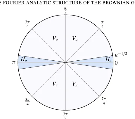
Definition 3.1(horizontal and vertical angles). Define the threshold angle
θu:=min
u−1/2,π4 .
Partition the angles[0,2π)usingθu into thehorizontal angles
Hu:= [0, θu] ∪ [π−θu, π+θu] ∪ [2π−θu,2π) and thevertical angles
Vu:= [0,2π)\Hu.
In other words Hu contains theθu neighborhoods of 0 andπ on the circle mod 2π andVu the π2−θu neighborhoods of π2 and32π respectively; seeFigure 2.
The proof will split into two cases in Sections3Band3C for bounding the Fourier transformµ(ξ)ˆ depending on whetherθ∈ Hu orθ ∈Vu:
(1) Section 3Bconcerns anglesθ∈ Hu, that is, close to horizontal directions 0 orπ, and as mentioned in theIntroductionour main hope here is that the smallness (with respect tou−1/2) of the diffusion componentbWt will help us in transferring the decay of Lebesgue measure to the decay ofµˆ. This is where Itô’s lemma (seeLemma 2.3) becomes crucial as it can be applied to the process f(Xt) with the function f(x)=exp(i x).
π
2
π
4
u−1/2
0
7π 4 3π
2 5π
4
π
3π 4
Vu Vu
Vu Vu
[image:10.500.138.369.49.252.2]Hu Hu
Figure 2. Splitting of[0,2π)to horizontal anglesHuand the vertical anglesVu.
It turns out that in both Sections3Band3Cwe only obtain decay of the Fourier transformµ(ˆ k)fork in anε-gridεZ2for all smallε >0. Here the randomness will depend onε >0 but thanks to an argument also used by Kahane[1985b], one can pass from this information to the full decay almost surely. See Section 3Dfor the details.
Let us now proceed to bound| ˆµ(ξ)|. In both Sections3Band 3Cbelow we will end up bounding trigonometric functions with respect toθu and for this purpose we will need the following standard bounds, which we record here for convenience:
Lemma 3.2(trigonometric bounds). We have the following bounds:
(1) If θ∈Hu,then
|sinθ|6u−1/2 and |cosθ|>√1 2. (2) If θ∈Vu,then
|sinθ|>minnπ2u−1/2,√1 2
o
.
Proof.Forα∈
0,π2
we have that both cosine and sine are nonnegative. Moreover, here π2α6sinα6α. Thus forθ∈ [0, θu]we have
sinθ 6θ 6θu6u−1/2 and cosθ>cosθu>cosπ4 =√1 2.
and forθ∈ θu,π
2
as sinπ4 =√1
2 we obtain
sinθ >minnπ2u−1/2,√1 2
o
.
This gives the claim as we may reduce the estimates back to the estimates forθ∈
0,π2
by using standard
3B. Horizontal angles. Whenθ∈Hu we will first obtain the following estimate onε-grids:
Lemma 3.3. Fixε >0. Almost surely there exists a random constant Cω>0such that for any k= u(cosθ,sinθ)∈εZ2\ {0}withθ ∈Hu we have
| ˆµ(k)|6Cω|k|−1/2.
Givenξ=u(cosθ,sinθ)∈R2\ {0}and a realisation(Wt), define a random variableT=Tω(ξ)∈ [0,1], to be the minimum value oft∈ [0,1]such that
Xt =
−2πdu(cosθ+W1sinθ)e ifX1>0,
−2πbu(cosθ+W1sinθ)c ifX1<0.
Such a timeT exists almost surely since X0=0 and Xt is almost surely continuous (since Wt is almost surely continuous). Splitting the integral of Zt up into “complete rotations” and “what is left over”, one obtains
Z 1
0
Ztdt= Z T
0
Ztdt+ Z 1
T Ztdt.
For the integral over[T,1]we get the following estimate.
Lemma 3.4. Almost surely there exists a random constant Cω>0such that for anyξ=u(cosθ,sinθ)∈ R2\ {0}withθ ∈Hu we have
Z 1
T Ztdt
6
Cω|ξ|−1/2.
Proof. SinceWt is almost surely continuous, there almost surely exists a random constantMω>1 such thatWt ∈ [−Mω,Mω]for allt∈ [0,1]. Define the real-valued process
Yt :=u(tcosθ+Wtsinθ),
so Xt = −2πYt. SupposeX1>0. In this caseYT = dY1e60 and soY1+1>YT >Y1. Moreover, when X1<0 we haveYT = bY1c>0 andY1>YT>Y1−1. Thus no matter what the sign of X1is, we always have almost surely
u(cosθ+W1sinθ)+1>u(Tcosθ+WTsinθ)>u(cosθ+W1sinθ)−1.
Therefore, in the case cosθ >0 we obtain
T >1+W1 sinθ cosθ −WT
sinθ cosθ −
1 ucosθ, and when cosθ <0 we have
T >1+W1 sinθ cosθ −WT
sinθ cosθ +
1 ucosθ. Sinceu∈Hu,Lemma 3.2together withWt∈ [−Mω,Mω]yields
T >1−2 √
2Mωu−1/2− √
Recalling Mω>1 this gives Z 1 T Ztdt
6 Z 1 T
|Zt|dt=1−T 64Mωu−1/2
as required.
We now estimate the integral over[0,T], which is where Itô calculus comes into play.
Lemma 3.5. Fixε >0. Almost surely there exists a random constant Cω>0such that for any k= u(cosθ,sinθ)∈εZ2\ {0}withθ ∈Hu we have
Z T 0 Ztdt
6
Cω|k|−1/2.
To prove Lemma 3.5, we first need to compute the higher-order moments of the random variable RT
0 Ztdt.
Lemma 3.6. For any p∈Nandξ=u(cosθ,sinθ)∈R2\ {0}withθ∈ Hu,the(2p)-th moment satisfies
E Z T 0 Ztdt
2p
613p1/24p|ξ|−p.
Proof. Recall that
Xt = −2πu(tcosθ+Wtsinθ)
is an Itô drift-diffusion process satisfying the stochastic differential equation
d Xt =b dt+σd Wt
for deterministic and time-independent coefficientsb= −2πucosθ andσ = −2πusinθ. Writing
f(x):=exp(i x), x∈R,
we have Zt = f(Xt), f0(x)=iexp(i x)and f00(x)= −exp(i x). Thus by complex Itô’s lemma (see
Lemma 2.3) we havePalmost surely
f(XT)− f(X0)=(bi−σ2/2) Z T
0
f(Xt)dt+σi Z T
0
f(Xt)d Wt. (3-2)
Note thatTω61 is random and onlyF1measurable; thus it is not a stopping time. However, asLemma 2.3 is givenpathwise, that is,Palmost surely Itô’s lemma holds for any timeT >0, then asTωisPalmost surely well-defined, we have (3-2) almost surely. Since X0 and XT are 2π multiples of integers by definition, we have f(XT)= f(X0)=1. Thus(3-2)gives
Z T
0
f(Xt)dt= −
σi bi−σ2/2
Z T
0
f(Xt)d Wt
Sincebandσ are deterministic, this yields that the(2p)-th moment satisfies
E Z T 0
f(Xt)dt 2p = σi bi−σ2/2
2p E Z T 0
Applying the Burkholder–Davis–Gundy inequality (seeLemma 2.4) for the process cosXt gives E Z T 0
cosXtd Wt 2p 6E sup 06s61
Z s 0
cosXtd Wt
2p
62p10p E
Z 1
0
cos2Xtdt p
62p10p
since cos261. Similar application for the process sinXt gives
E Z T 0
sinXtd Wt
2p
62p10p.
By Euler’s formula, we can write f(Xt)=cosXt+isinXt and so
Z T
0
f(Xt)d Wt = Z T
0
cosXtd Wt+i Z T
0
sinXtd Wt.
Hence E Z T 0
f(Xt)d Wt 2p =E Z T 0
cosXtd Wt 2 + Z T 0
sinXtd Wt 2p 6E 2p Z T 0
cosXtd Wt
2p
+2p
Z T 0
sinXtd Wt
2p
=2p
E Z T 0
cosXtd Wt 2p +E Z T 0
sinXtd Wt
2p
62p4p10p.
Moreover, asθ ∈Hu we have byLemma 3.2that cos2θ >12 and sin2θ6u−1. Hence
σi bi−σ2/2
2 = σ 2
b2+σ4/4 6
σ2 b2 =
4π2u2sin2θ 4π2u2cos2θ =
sin2θ cos2θ 62u
−1.
Therefore, E Z T 0
f(Xt)dt
2p
64p10p4pθ2p613p1/24pu−p.
as required.
Proof of Lemma 3.5.Fixε >0. Then for allk∈εZ2\ {0}define the random variable I(k):=
Z T
0 Ztdt
·χA(k),
whereχA is the indicator function on the set
A:=ξ=u(cosθ,sinθ)∈R2\ {0} :θ∈ Hu .
Note that I(k)is well-defined and finite since RT
0 Ztdt
61 by|exp(i x)| =1.Lemma 3.6now yields for anyk∈εZ2\ {0}and p∈Nthat
as whenk∈/ Awe haveI(k)≡0. Write pk= blog|k|c. Then
E X
k∈εZ2\{0}
|k|−3 |I(k)|
2pk
13p1k/24pk|k|−pk 6 X
k∈εZ2\{0}
|k|−3<∞.
This means that the summands tend to 0 almost surely as|k| → ∞and so we can find a random constant Cω>0 such that for all k∈εZ2\ {0}we have
|k|−3 |I(k)|
2pk
13p1k/24pk|k|−pk
6Cω.
Therefore, by possibly makingCωbigger we obtain
|I(k)|6Cω|k|−1/2.
This holds for eachk∈εZ2\ {0}, so by the definition of I(k)we have wheneverk=u(cosθ,sinθ)∈
εZ2\ {0}withθ∈ Hu that
Z T
0 Ztdt
6
Cωu−1/2
as claimed.
We are now in position to complete the proof ofLemma 3.3.
Proof of Lemma 3.3.Fixε >0. By the splitting ˆ
µ(ξ)=
Z 1
0
Ztdt= Z T
0
Ztdt+ Z 1
T Ztdt
and Lemmas3.4and3.5, we have that almost surely there exists a constantCω >0 such that for all
k=u(cosθ,sinθ)∈εZ2\ {0}withθ ∈Hu we have
| ˆµ(k)|6
Z T
0 Ztdt
+
Z 1
T Ztdt
6
Cω|k|−1/2
as required.
3C. Vertical angles. In this section we apply Kahane’s work to obtain Fourier decay estimates when
θ ∈Vu.
Lemma 3.7. Fixε >0. Almost surely there exists a random constant Cω>0such that for any k= u(cosθ,sinθ)∈εZ2\ {0}withθ ∈Vuwe have
| ˆµ(k)|6Cω|k|−1/2plog|k|.
Let us discuss a few estimates obtained in[Kahane 1985b]. Letν be the push-forward of Lebesgue measure on[0,1]under the mapt7→Wt; that is,νis the Brownian image of Lebesgue measure. Kahane established the following:
Theorem 3.8[Kahane 1985b, page 255]. Almost surely
The key ingredient for the proof ofTheorem 3.8was based on establishing the following bound for the higher moments:
Lemma 3.9[Kahane 1985b, page 254, estimate (2)]. There exists a constant C>0such that for any
v∈R\ {0}and any p∈Nwe have
E| ˆν(v)|2p6Cppp|v|−2p.
We can useLemma 3.9to give a bound on the higher moments in our setting, but with the price that the exponent will increase from−2pto−p.
Lemma 3.10. There exists a constant C >0such that for any p∈Nandξ=u(cosθ,sinθ)∈R2\ {0} withθ∈Vuthe(2p)-th moment satisfies
E| ˆµ(ξ)|2p6Cppp|ξ|−p.
Proof. Writet=(t1, . . . ,tp)∈ [0,1]panddt as the Lebesgue measure on[0,1]p. Givent,s∈ [0,1]p, we define
ϕ(t,s):=
p X
k=1
(tk−sk), ψ(t,s):= p X
k=1
(Wtk−Wsk), and 9(t,s):=E|ϕ(t,s)|
2.
By the definition ofµθ,µand the Fourier transform, and using the fact that the multivariate process
X(t,s):= −2πcos(θ)ϕ(t,s)−2πsin(θ)ψ(t,s)
is Gaussian with mean−2πcos(θ)ϕ(t,s)and variance 4π2sin2(θ)9(t,s), we have through Fubini’s theorem and the formula for the characteristic function that
E| ˆµ(ξ)|2p=E
Z
[0,1]p
Z
[0,1]p
exp −2πi u cos(θ)ϕ(t,s)+sin(θ)ψ(t,s)dtds
=
Z
[0,1]p
Z
[0,1]pE
exp(i u X(t,s))dtds
=
Z
[0,1]p
Z
[0,1]p
exp −2πicos(θ)uϕ(t,s)−2π2|usin(θ)|29(t,s)dtds.
Thus by taking absolute values inside the integrals, and observing that|exp(i x)| =1 for anyx ∈R, we obtain
E| ˆµ(ξ)|2p6
Z
[0,1]p
Z
[0,1]p
exp(−2π2|usin(θ)|29(t,s))dtds. (3-3)
On the other hand, by doing the expansion again for the Fourier transformνˆ of the image measureνat
v:=usin(θ)∈R\ {0}we see that
E| ˆν(v)|2p=E
Z
[0,1]p
Z
[0,1]p
exp(−2πivψ(t,s))dtds=
Z
[0,1]p
Z
[0,1]p
exp(−2π2v29(t,s))dtds,
which is equal to(3-3). Thus byLemma 3.9we have
Sinceθ ∈Vuwe have|sinθ|>min n
2
πu−1/2,√12 o
. When|sinθ|>√1
2 we obtain
Cppp|v|−2p6(2C)pppu−2p6(2C)pppu−p.
On the other hand, if|sinθ|> 2
πu−1/2we have
Cppp|v|−2p6Cppp(2u−1/2/π)−2pu−2p6(Cπ2/4)pppu−p.
Now we can complete the proof ofLemma 3.7for vertical directions:
Proof of Lemma 3.7.Fixε >0. Then for allk=u(cosθ,sinθ)∈εZ2\ {0}define the random variable F(k):= ˆµ(k)χB(k),
where
B:=ξ=u(cosθ,sinθ)∈R2\ {0} :θ∈Vu .
Now F(k)is a well-defined finite random variable as| ˆµ(k)|61 for anyk. FromLemma 3.10we obtain for anyk∈εZ2\ {0}and p∈Nthat
E|F(k)|2p6Cppp|k|−p.
Write pk= blog|k|c. Then
E X
k∈εZ2\{0}
|k|−3 |F(k)|
2pk
Cpkpkpk|k|−pk 6 X
k∈εZ2\{0}
|k|−3<∞.
This means that the summands tend to 0 almost surely as|k| → ∞and so we can find a random constant Cω>0 such that for all k∈εZ2\ {0}we have
|k|−3 |F(k)|
2pk
Cpkp
kpk|k|−pk 6
Cω.
Thus possibly makingCωbigger, this yields
|F(k)|6Cω|k|−1/2plog|k|.
Now this holds for eachk∈εZ2\{0}, so by the definition ofF(k)we have, wheneverk=u(cosθ,sinθ)∈
εZ2\ {0}withθ∈Vu, that
| ˆµ(k)|6Cω|k|−1/2plog|k|
as claimed.
3D. From lattices toR2. We can now complete the proof of the main theorem. For this purpose, we need the following comparison lemma used by Kahane that allows us to pass from convergence on lattices for Fourier transforms to the whole space:
Lemma 3.11 [Kahane 1985b, Lemma 1, page 252]. Supposeτ is a measure onR2 with support in
(−1,1)2. Supposeϕ, ψ:(0,∞)→(0,∞)are decreasing as t→ ∞with the doubling properties
If the Fourier transform of τ along the integer latticeZ2satisfies
| ˆτ(n)| =O ϕ(
|n|)
ψ(|n|)
as|n| → ∞,
then
| ˆτ(ξ)| =O
ϕ(
|ξ|)
ψ(|ξ|)
as|ξ| → ∞.
Proof of Theorem 1.3.Combining Lemmas3.7and3.3we have that for anyε >0, almost surely, there exists some random constantCω>0 such that for any k=u(cosθ,sinθ)∈εZ2\ {0}we have
| ˆµ(k)|6Cω|k|−1/2plog|k|. (3-4)
Define a measureτε onR2 such that
ˆ
τε(ξ):= ˆµ(εξ), ξ∈R2.
By the almost sure continuity of Wt, we have that there exists a random constant Mω>0 such that the diameter of the support ofµis at most Mωalmost surely. Taking an intersection of the events that(3-4) holds forε=1/nover alln∈Nallows us to find a randomε=εω>0 such that µis supported on a set of diameter strictly less than 1/εand(3-4)holds almost surely with thisε. This guarantees that the measureτε is supported on(−1,1)2and so applyingLemma 3.11with the measureτ =τε and the maps
ϕ(t):=plogt andψ(t):=t1/2gives the claim.
Acknowledgements
We thank Tuomas Orponen for useful discussions during the preparation of this manuscript. We are also grateful to an anonymous referee for comments and suggestions which improved the focus of the paper. Finally, we thank The Hebrew University of Jerusalem and The University of Manchester for hosting us for research visits during the writing of this paper.
References
[Adler 1977] R. J. Adler,“Hausdorff dimension and Gaussian fields”,Ann. Probability5:1 (1977), 145–151. MR Zbl [Beffara 2008] V. Beffara,“The dimension of the SLE curves”,Ann. Probab.36:4 (2008), 1421–1452. MR Zbl
[Bluhm 1998] C. Bluhm,“On a theorem of Kaufman: Cantor-type construction of linear fractal Salem sets”,Ark. Mat.36:2 (1998), 307–316. MR Zbl
[Burkholder et al. 1972] D. L. Burkholder, B. J. Davis, and R. F. Gundy, “Integral inequalities for convex functions of operators on martingales”, pp. 223–240 inProceedings of the Sixth Berkeley Symposium on Mathematical Statistics and Probability, II: Probability theory(Berkeley, CA, 1970/1971), Univ. California Press, Berkeley, CA, 1972. MR Zbl
[Chan et al. 2016] V. Chan, I. Łaba, and M. Pramanik,“Finite configurations in sparse sets”,J. Anal. Math.128(2016), 289–335. MR Zbl
[Davenport et al. 1963] H. Davenport, P. Erd˝os, and W. J. LeVeque,“On Weyl’s criterion for uniform distribution”,Michigan Math. J.10(1963), 311–314. MR Zbl
[Ekström et al. 2015] F. Ekström, T. Persson, and J. Schmeling,“On the Fourier dimension and a modification”,J. Fractal Geom.
[Fouché and Mukeru 2013] W. L. Fouché and S. Mukeru,“On the Fourier structure of the zero set of fractional Brownian motion”,Statist. Probab. Lett.83:2 (2013), 459–466. MR Zbl
[Fraser et al. 2014] J. M. Fraser, T. Orponen, and T. Sahlsten,“On Fourier analytic properties of graphs”,Int. Math. Res. Not.
2014:10 (2014), 2730–2745. MR Zbl
[Jordan and Sahlsten 2016] T. Jordan and T. Sahlsten,“Fourier transforms of Gibbs measures for the Gauss map”,Math. Ann.
364:3-4 (2016), 983–1023. MR Zbl
[Kahane 1966a] J.-P. Kahane, “Images browniennes des ensembles parfaits”,C. R. Acad. Sci. Paris Sér. A-B263(1966), A613–A615. MR Zbl
[Kahane 1966b] J.-P. Kahane, “Images d’ensembles parfaits par des séries de Fourier gaussiennes”,C. R. Acad. Sci. Paris Sér. A-B263(1966), A678–A681. MR Zbl
[Kahane 1985a] J.-P. Kahane,“Ensembles aléatoires et dimensions”, pp. 65–121 inRecent progress in Fourier analysis(El Escorial, 1983), edited by I. Peral and J. L. Rubio de Francia, North-Holland Math. Stud.111, North-Holland, Amsterdam, 1985. MR Zbl
[Kahane 1985b] J.-P. Kahane,Some random series of functions, 2nd ed., Cambridge Studies in Advanced Mathematics5, Cambridge University Press, 1985. MR Zbl
[Kahane 1993] J.-P. Kahane, “Fractals and random measures”,Bull. Sci. Math.117:1 (1993), 153–159. MR Zbl
[Karatzas and Shreve 1991] I. Karatzas and S. E. Shreve,Brownian motion and stochastic calculus, 2nd ed., Graduate Texts in Mathematics113, Springer, 1991. MR Zbl
[Kaufman 1980] R. Kaufman,“Continued fractions and Fourier transforms”,Mathematika27:2 (1980), 262–267. MR Zbl [Kaufman 1981] R. Kaufman,“On the theorem of Jarník and Besicovitch”,Acta Arith.39:3 (1981), 265–267. MR Zbl [Körner 2011] T. W. Körner,“Hausdorff and Fourier dimension”,Studia Math.206:1 (2011), 37–50. MR Zbl
[Łaba and Pramanik 2009] I. Łaba and M. Pramanik,“Arithmetic progressions in sets of fractional dimension”,Geom. Funct. Anal.19:2 (2009), 429–456. MR Zbl
[Mattila 1995] P. Mattila,Geometry of sets and measures in Euclidean spaces: fractals and rectifiability, Cambridge Studies in Advanced Mathematics44, Cambridge University Press, 1995. MR Zbl
[Mattila 2015] P. Mattila, Fourier analysis and Hausdorff dimension, Cambridge Studies in Advanced Mathematics150, Cambridge University Press, 2015. MR Zbl
[McKean 1955] H. P. McKean, Jr.,“Hausdorff–Besicovitch dimension of Brownian motion paths”,Duke Math. J.22(1955), 229–234. MR Zbl
[Peres and Sousi 2016] Y. Peres and P. Sousi,“Dimension of fractional Brownian motion with variable drift”,Probab. Theory Related Fields165:3-4 (2016), 771–794. MR Zbl
[Perkins 1981] E. Perkins,“The exact Hausdorff measure of the level sets of Brownian motion”,Z. Wahrsch. Verw. Gebiete58:3 (1981), 373–388. MR Zbl
[Peškir 1996] G. Peškir, “On the exponential Orlicz norms of stopped Brownian motion”,Studia Math.117:3 (1996), 253–273. MR Zbl
[Queffélec and Ramaré 2003] M. Queffélec and O. Ramaré, “Analyse de Fourier des fractions continues à quotients restreints”,
Enseign. Math.(2)49:3-4 (2003), 335–356. MR Zbl
[Salem 1951] R. Salem,“On singular monotonic functions whose spectrum has a given Hausdorff dimension”,Ark. Mat.1
(1951), 353–365. MR Zbl
[Shieh and Xiao 2006] N.-R. Shieh and Y. Xiao,“Images of Gaussian random fields: Salem sets and interior points”,Studia Math.176:1 (2006), 37–60. MR Zbl
[Shmerkin 2017] P. Shmerkin,“Salem sets with no arithmetic progressions”,Int. Math. Res. Not.2017:7 (2017), 1929–1941. MR
[Taylor 1953] S. J. Taylor,“The Hausdorffα-dimensional measure of Brownian paths inn-space”,Proc. Cambridge Philos. Soc.
49(1953), 31–39. MR Zbl
Received 28 Mar 2016. Revised 19 Jul 2017. Accepted 5 Sep 2017.
JONATHANM. FRASER: [email protected]
School of Mathematics and Statistics, University of St Andrews, St Andrews, United Kingdom
TUOMASSAHLSTEN: [email protected]
School of Mathematics, University of Manchester, Manchester, United Kingdom
msp.org/apde
EDITORS
EDITOR-IN-CHIEF
Patrick Gérard
Université Paris Sud XI Orsay, France
BOARD OFEDITORS
Nicolas Burq Université Paris-Sud 11, France
Massimiliano Berti Scuola Intern. Sup. di Studi Avanzati, Italy
Sun-Yung Alice Chang Princeton University, USA
Michael Christ University of California, Berkeley, USA
Charles Fefferman Princeton University, USA
Ursula Hamenstaedt Universität Bonn, Germany
Vaughan Jones U.C. Berkeley & Vanderbilt University
Vadim Kaloshin University of Maryland, USA
Herbert Koch Universität Bonn, Germany
Izabella Laba University of British Columbia, Canada
Gilles Lebeau Université de Nice Sophia Antipolis, France
Richard B. Melrose Massachussets Inst. of Tech., USA
Frank Merle Université de Cergy-Pontoise, France
William Minicozzi II Johns Hopkins University, USA
Clément Mouhot Cambridge University, UK
Werner Müller Universität Bonn, Germany
Gilles Pisier Texas A&M University, and Paris 6
Tristan Rivière ETH, Switzerland
Igor Rodnianski Princeton University, USA
Wilhelm Schlag University of Chicago, USA
Sylvia Serfaty New York University, USA
Yum-Tong Siu Harvard University, USA
Terence Tao University of California, Los Angeles, USA
Michael E. Taylor Univ. of North Carolina, Chapel Hill, USA
Gunther Uhlmann University of Washington, USA
András Vasy Stanford University, USA
Dan Virgil Voiculescu University of California, Berkeley, USA
Steven Zelditch Northwestern University, USA
Maciej Zworski University of California, Berkeley, USA
PRODUCTION
Silvio Levy, Scientific Editor
See inside back cover ormsp.org/apdefor submission instructions.
The subscription price for 2018 is US $275/year for the electronic version, and $480/year (+$55, if shipping outside the US) for print and electronic. Subscriptions, requests for back issues from the last three years and changes of subscriber address should be sent to MSP.
Analysis & PDE (ISSN 1948-206X electronic, 2157-5045 printed) at Mathematical Sciences Publishers, 798 Evans Hall #3840, c/o Uni-versity of California, Berkeley, CA 94720-3840, is published continuously online. Periodical rate postage paid at Berkeley, CA 94704, and additional mailing offices.
APDE peer review and production are managed by EditFlow®from MSP.
PUBLISHED BY
mathematical sciences publishers nonprofit scientific publishing
http://msp.org/
A
NALYSIS
& PDE
Volume 11
No. 1
2018
1 Analytic torsion, dynamical zeta functions, and the Fried conjecture
SHUSHEN
75 Existence theorems of the fractional Yamabe problem
SEUNGHYEOKKIM, MONICAMUSSOand JUNCHENGWEI
115 On the Fourier analytic structure of the Brownian graph
JONATHANM. FRASERand TUOMASSAHLSTEN
133 Nodal geometry, heat diffusion and Brownian motion
BOGDANGEORGIEVand MAYUKHMUKHERJEE
149 A normal form à la Moser for diffeomorphisms and a generalization of Rüssmann’s translated curve theorem to higher dimensions
JESSICAELISAMASSETTI
171 Global results for eikonal Hamilton–Jacobi equations on networks
ANTONIOSICONOLFIand ALFONSOSORRENTINO
213 High-frequency approximation of the interior Dirichlet-to-Neumann map and applications to the transmission eigenvalues
GEORGIVODEV
237 Hardy–Littlewood inequalities on compact quantum groups of Kac type
SANG-GYUNYOUN