Optimizing countershading camouflage
Innes C. Cuthilla, N. Simon Sangheraa, Olivier Penacchiob, P. George Lovelld, Graeme D. Ruxtonc and Julie M. Harrisb
a School of Biological Sciences, Life Sciences Building, 24 Tyndall Avenue, Bristol
BS8 1TQ, UK
b School of Psychology and Neuroscience, South Street, University of St Andrews, St
Andrews, Fife KY16 9JP UK
c School of Biology, Dyers Brae, University of St Andrews, St Andrews, Fife KY16
9TH UK
d Division of Psychology, Social and Health Sciences, Abertay University, Dundee,
DD1 1HG, UK
Corresponding author: Innes Cuthill. Address as above. Tel.: +44 117 394 1175 E-mail: [email protected]
Classification: BIOLOGICAL SCIENCES: Ecology
Abstract
Countershading, the widespread tendency of animals to be darker on the side that receives strongest illumination, has classically been explained as an adaptation for camouflage: obliterating cues to 3D shape and enhancing background matching. However, there have only been two quantitative tests of whether the patterns observed in different species match the optimal shading to obliterate 3D cues, and no tests of whether optimal countershading actually improves concealment or survival. We use a mathematical model of the light field to predict the optimal countershading for
concealment that is specific to the light environment, then test this with
correspondingly patterned model “caterpillars” exposed to avian predation in the field. We show that the optimal countershading is strongly illumination dependent. A
Significance Statement
\body Introduction
Many animals, across diverse taxa and habitats, are darker on their dorsal than ventral side (1-8). One of the oldest theories of animal camouflage (9-13) suggests that this ‘countershading’ has evolved to cancel the dorso-ventral gradient of illumination across the body, thus obliterating cues to 3D form and enhancing background
matching. Indeed, so common are dorso-ventral gradients of pigmentation that Abbott Thayer branded his explanation as “The law which underlies protective coloration” (12). Countershading also became one of the most popular early tactics in military camouflage (14, 15). Yet somewhat ironically, given that the theory was inspired by observations of nature, a role in biological camouflage remains equivocal. The current paper uses predation rate to test directly whether countershading affects detectability and, for the first time, the degree to which the pattern has to be tightly matched to the illumination conditions to be effective.
Assessments of coat pattern in relation to positional behavior and body size in
optimized. One problem is that the predictions for UV protection are very similar to those for optimized camouflage (17-20). So without measurement of predation rates on animals with or without the observed coloration, we cannot tell if there is a causal effect on detectability. .
While some tests with artificial prey show reduced avian predation rates on two-tone, dorsally darker treatments (21-24), the relationship between the color contrasts in these experiments and the predicted optima are unknown. We have recently filled this important gap by using a general theory of optimal countershading to derive the predicted optimal patterns for different weather conditions at a specific location, time of year and day (25). Modeling of the light field shows that a sharp transition between dark and light, as used in previous experimental studies, provides optimal
caterpillar-like prey with these putatively optimized patterns, under different illumination conditions.
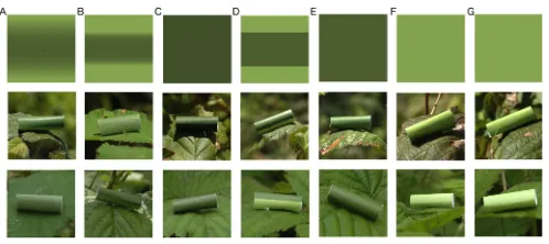
We produced large numbers of cylindrical paper ‘caterpillars’ with different dorso-ventral color gradients. Two were designed to counterbalance direct sun or diffuse illumination and so each should be the optimal countershading in its own, and only its own, light environment (Fig. 1). Control patterns were uniform or two-tone. We then attached these to vegetation, in a randomized block design, on both sunny and cloudy days, directly in sun or in shade. We predicted that countershading optimized for the prey-specific illumination conditions would suffer lower predation rates by wild birds than those with countershading optimized for different lighting, or with no
countershading at all.
Results
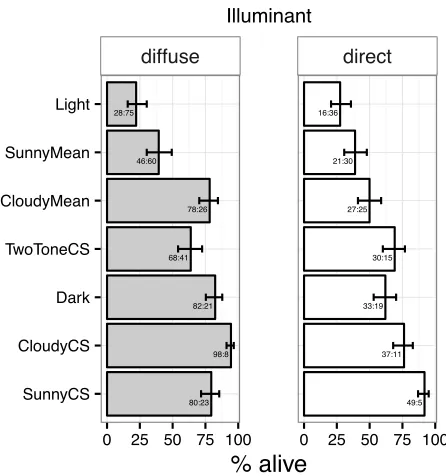
We can model illumination conditions at the level of the individual prey item or at the level of the block. The former provided a better fit to the data (AIC = 1166.8 vs 1179.2, both models with treatment and illumination condition and their interaction as fixed effects, with block as a random effect; see Methods). The results that follow (and shown in Figure 2) therefore refer to the former model structure.
= 171.39, d.f. = 6, p < 0.0001), with the countershaded treatment for cloudy
conditions (CloudyCS) surviving significantly better than all other treatments (Fig. 2; Table 1, grey lower left triangle). Next best surviving, and similar to each other, were Dark, CloudyMean and SunnyCS. The sharp-boundary two-tone countershaded treatment (TwoToneCS) survived next best, significantly worse than CloudyCS, SunnyCS and Dark, similar to CloudyMean, and significantly better than SunnyMean and Light.
For direct illumination, treatment was also significant (χ2 = 65.11, d.f. = 6, p < 0.0001), with the countershaded treatment for sunny conditions (SunnyCS) surviving best, significantly better than all treatments including, very marginally, the
countershaded treatment for cloudy conditions (Fig. 2; Table 1, upper right triangle). CloudyCS, TwoToneCS and Dark survived next best, with CloudyCS surviving significantly better than CloudyMean, SunnyMean and Light. TwoToneCS and Dark were also intermediate, but only significantly worse than the best-surviving SunnyCS and only significantly better than the worst-surviving Light.
We can test directly whether the dependence of survival on illumination differed between the SunnyCS and CloudyCS treatments in two ways. First by repeating the analysis for only these two patterns: the treatment by illumination interaction was significant (χ2 = 12.218, d.f. = 1, p = 0.0005). Second, by creating a new binary
was the main effect of illumination (χ2 = 0.16, d.f. = 1, p = 0.6861). Only the main effect of matching was (χ2 = 14.20, d.f. = 1, p < 0.0001).
Discussion
Our results show that countershading provides concealment benefits, but the key novel result is that optimal countershading is strongly dependent upon illumination conditions. The indirect illumination optimum (CloudyCS) did best when prey were in indirect illumination and the direct illumination optimum (SunnyCS) did best when prey were in direct illumination. Therefore the optimal patterns for camouflage, measured here, match the comparative evidence from Allen et al. (1), where species that frequented open lighting environments and/or lived closer to the equator had a steeper gradient of countershading. These results also support observations of countershading being more obvious in relatively diurnal species, in those living in deserts, and found less often in tundra-living artiodactyls (7).
There is no evidence that having the “wrong” countershading pattern has asymmetric costs. CloudyCS was compromised in direct sun as much as SunnyCS was
compromised in shade. However, these results alone do not allow us to draw strong conclusions about the single best countershaded pattern to pick when a prey species is subject to both direct and indirect illumination. This would depend on the relative probability of being viewed by a predator under each type of lighting condition, something that is dependent upon predator behavior as well as weather variability.
background matching color for a flat prey (Dark). However, previous experiments that used a two-tone prey (e.g. 21, 22, 23, 24) showed an advantage for
countershading over uniform background-matching dark green. As mentioned in the introduction, it was not the case that all these experiments were carried out on sunny days, nor were the prey carefully aligned to the sun (as in the present study, and necessary for countershading to function in direct illumination; 18). It is possible that, given that the prey were made from pastry dough, the boundary was smudged by handling and so a partial gradient (not quantified) may have been created. Otherwise, the higher survival of two-tone prey in those experiments may have in fact resulted from a combination of background matching and disruptive coloration (9, 13, 26, 27).
animal, optimal countershading can only be achieved by orienting towards the sun because an optimal symmetrical camouflage requires an illumination field that is symmetrical with respect to the animal (18). That an animal such as a caterpillar would move with the time of day so as to maintain equal illumination on both sides of its body is plausible, but untested. Maintaining such an orientation is certain to have costs, so it is inevitable that camouflage through countershading is traded off against factors such as feeding efficiency, what the substrate allows, the need to move, and effects on thermoregulation (18). How such trade-offs affect behavior are completely unexplored, but must be if we are to understand fully the interaction between light environment, orientation behavior and coloration.
Materials and Methods
The overall strategy was to (i) model, under different weather conditions, the pattern of light reflected from a uniform grey cylinder lying on a uniform grey plane, (ii) use this to compute the pattern of reflectance on the cylinder that would both obliterate any gradient created by the illumination (i.e. cues to 3D shape) and match the
background, then (iii) recolor the greys to match the average green of bramble leaves, the actual ‘plane’ on which the artificial cylindrical caterpillars would lie in a field experiment. The color was chosen so that it would produce a match to average bramble leaf green for avian vision.
Target construction
RADIANCE (28). This is ray-tracing software that enables 3D modeling of scenes under realistic illumination conditions, with the position of the sun and
presence/absence of clouds, as well as the reflectance of objects and backgrounds, under control of the user. Radiance uses standard descriptors of the spatial distribution of daylight provided by the Commission Internationale d’Eclairage (29), based on user-supplied latitude, longitude, date, time and cloud cover; the accuracy of the output has been validated by Ruppertsberg and Bloj (30).
We modeled the prey item as a uniform grey cylinder, lying horizontally with its axis facing the sun at 15:00 h GMT in Bristol (51.45° N, 2.60° W), the time and place of all experimental blocks. This exercise was repeated for every date on which specific blocks were run. The aim was to produce an ‘optimal’ pattern of counter-shading that would cancel the shading difference across the cylinder caused by the interaction between animal shape and direction of light from the sky (be it sunny or cloudy). We computed the irradiance falling on the cylinder under two conditions: sunny
(cloudless sky) and cloudy (100% cloud cover). The cylinder was assumed to be Lambertian, reflecting the light equally in every direction (i.e. matte with no specular reflection). Following Penacchio et al. (25), if 𝒊𝒓𝒓(𝒙) is the irradiance falling onto the
cylinder at location𝒙 and 𝒓𝒂𝒅𝒃𝒂𝒄𝒌𝒈𝒓𝒐𝒖𝒏𝒅 is the radiance of the background, the
reflectance of the body at the same location, 𝒓𝒆𝒇𝒍(𝒙), which both cancels out the
gradient of illumination and matches the background exactly is given by:
When the cylinder mainly receives direct light from the sun, a sharp transition
between the dark top and light underside is predicted (Fig. 1B). When the illumination is from the sky, with no direct sun (due to shading or cloud cover), the gradient from dark to light is shallower (Fig. 1A).
Color matching
The procedure above provided the change in color intensity for each treatment; the next step was to convert these grayscale models to colors that matched the
background. To obtain the colors necessary for background matching, 25 bramble leaves (each one from a separate plant) were collected from the field site and
The “average bramble leaf in avian color space” was based on spectrometry of both printed paper and bramble leaves, followed by color space modeling for the blue tit (Cyanistes caeruleus), which has color vision typical of the passerines seen foraging in the field site (33). Ten haphazardly chosen spots on each upper side of the 25 photographed bramble leaves were measured using a Zeiss MCS 230 diode array photometer (Carl Zeiss Group, Jena, Germany), with illumination by a Zeiss CLX 111 Xenon lamp held at 45° to normal to reduce specularity. Measurements were taken normal to the surface, from a ca. 2 mm area, recorded in 1 nm intervals from 300 to 700 nm, and expressed relative to a Spectralon 99% white reflectance standard (Labsphere, Congleton, UK). The reflectance data was multiplied by data on cone spectral sensitivities in Hart et al. (33) and a D65 irradiance spectrum (29) to obtain predicted photon catches for the blue tit single and double cones, as described previously (26, 27, 34).
Experimental design
There were seven treatments: the predicted optimal countershading for a sunny day (SunnyCS), the predicted optimal countershading for a cloudy day (CloudyCS), the darkest color of the countershaded treatments (Dark; equivalent to the background matching color for a flat object), the lightest color on the sunny countershaded treatment (Light), the mean of the sunny countershaded treatment (SunnyMean), the mean of the cloudy countershaded treatment (CloudyMean), and a two-tone
countershaded treatment (TwoToneCS) that had the colors of the Dark and Light treatment but with a sharp boundary rather than a gradient. The latter treatment was included because it is qualitatively similar to the type of countershading used in previous experiments, where dark and light green pastry dough have been stuck together (21-24).
For each experimental block, a sheet of targets was printed at a resolution of 600 dpi on a calibrated HP 2500 laserjet printer (Hewlett-Packard, Palo Alto, CA, USA) onto matte waterproof paper (Rite-in-the-Rain, Tacoma, WA, USA). Each target was a 2.5
1.5 cm dressmaking pin at an angle, at one end of the cylinder, through first the body of the mealworm and then the base of the cylinder and finally the leaf. In this way, the pin and mealworm were not visible from most angles of view. Cylinders (prey) were oriented so that their long axis faced the sun (or, when the sky was overcast, the position of the sun) and they were approximately horizontal, thus matching the modeled orientation.
The experiment had a randomized block design, with 14 blocks. There were 12 replicates per treatment per block in blocks one to nine, and 10 replicates per treatment per block in blocks 10 to 14; this difference was accidental, and of no consequence to the experiment. In any one block, a suitable bramble leaf was found and then a prey was selected at random by picking, whilst looking away, from a thoroughly mixed box of replicates. As each prey was attached to its leaf, its location was recorded on a map and a note made of whether it was directly illuminated by the sun or not. Each block took place in a different location in the public park Brandon Hill, Bristol, UK (51.4529° N, 2.6068° W), and open picnic areas of Leigh Woods Nature Reserve (51.4631° N, 2.6392° W) and Ashton Court park (51.4479° N,
European robin (Erithacus rubecula), dunnock (Prunella modularis), Eurasian wren (Troglodytes troglodytes) and Eurasian blackcap (Sylvia atricapilla).
Five of the blocks took place under overcast conditions (no direct sun) and nine on clear sunny days, with the sun shining unobscured by clouds for the duration of the block. The overcast days were reasonably interspersed across the experiment, being blocks 4, 5, 7, 8 and 14, with none taking place within the same week. Each block started at 2 pm GMT, taking ca. 45 min to place out all prey. The prey were checked from 1 h after the last had been placed out, with cylinders from which the mealworm had been completely or partially removed scored as ‘predated’. There were no prey taken by invertebrate predators (c.f. experiments taking place over longer periods, such as 26), but 11 prey could not be located. These missing values, were < 1% of the total and were not biased towards any one treatment (no more than three in any one treatment).
Analysis
multi-level, models fitted using the function glmer in the package lme4 (36) in R 3.0.2. Illumination conditions at the levels of block and prey could not be fitted within the same model, because on cloudy days all prey were in diffuse illumination, but the separate models could be compared for explanatory power with Akaike’s Information Criterion (AIC) (36).
Models had Bernoulli errors (binomial with 1 trial, alive or dead) with the fixed factors treatment (seven levels as described earlier) and illumination conditions (direct or diffuse illumination) and the random effect block (14 levels). Conventional hypothesis tests were by likelihood ratio test against a chi-squared distribution with degrees of freedom equal to the difference in degrees of freedom between models. For pair-wise tests following a significant treatment effect, the number of possible tests is greater than the degrees of freedom (six), so we adopted the following strategy. Comparisons of a priori interest at the time the experiment was designed (n=11) were tested using the False Discovery Rate procedure (37), which achieves a good balance between Type I and II errors (38). These were CloudyCS vs CloudyMean, CloudyCS vs Dark, CloudyCS vs Light, CloudyCS vs SunnyCS, SunnyCS vs CloudyMean, SunnyCS vs Dark, SunnyCS vs Light , Two-toneCS vs Dark, Two-toneCS vs Light, Two-toneCS vs CloudyCS and Two-toneCS vs SunnyCS. Other tests, of secondary interest, were tested with the Tukey procedure in the R package multcomp (39), controlling for all possible multiple comparisons within the seven treatments (n=21). Graphs were plotted with the lattice package (40).
We thank Tim Caro and two anonymous referees for their constructive comments. The research was funded by grants from the Biotechnology & Biological Sciences Research Council, UK, to JMH, GDR, ICC and PGL. ICC thanks the
Wissenschaftskolleg zu Berlin for support during part of the study. The experiment was approved by the University of Bristol Animal Welfare & Ethical Review Body.
References
1. Allen WL, Baddeley R, Cuthill IC, Scott-Samuel NE (2012) A quantitative test of the predicted relationship between countershading and lighting environment. Am Nat180(6):762-776.
2. Caro T (2009) Contrasting coloration in terrestrial mammals. Phil Trans R Soc B364(1516):537-548.
3. Caro T, Beeman K, Stankowich T, Whitehead H (2011) The functional significance of colouration in cetaceans. Evol Ecol25(6):1231-1245. 4. Caro TM (2005) The adaptive significance of coloration in mammals.
BioScience55:125-136.
5. Kamilar JM (2009) Interspecific variation in primate countershading: Effects of activity pattern, body mass, and phylogeny. Int J Primatol30(6):877-891. 6. Stoner CJ, Bininda-Emonds ORP, Caro T (2003) The adaptive significance of
coloration in lagomorphs. Biol J Linn Soc79(2):309-328.
7. Stoner CJ, Caro TM, Graham CM (2003) Ecological and behavioral correlates of coloration in artiodactyls: systematic analyses of conventional hypotheses.
Behav Ecol14(6):823-840.
9. Cott HB (1940) Adaptive Coloration in Animals (Methuen & Co. Ltd., London).
10. Klein A, Mottram JC (1919) Military camouflage. Nature103:364. 11. Poulton EB (1890) The Colours of Animals: Their Meaning and Use.
Especially Considered in the Case of Insects. Second Edition (Kegan Paul, Trench Trübner, & Co. Ltd, London).
12. Thayer AH (1896) The law which underlies protective coloration. The Auk
13:477-482.
13. Thayer GH (1909) Concealing-Coloration in the Animal Kingdom: An Exposition of the Laws of Disguise Through Color and Pattern: Being a
Summary of Abbott H. Thayer's Discoveries. (Macmillan, New York). 14. Behrens RR (1988) The theories of Abbott H. Thayer: Father of camouflage.
Leonardo21:291-296.
15. Behrens RR (2002) False Colors: Art, Design and Modern Camouflage
(Bobolink Books, Dysart, Iowa).
16. Kamilar JM, Bradley BJ (2011) Countershading is related to positional behavior in primates. J Zool283:227-233.
17. Kiltie RA (1988) Countershading: Universally deceptive or deceptively universal? TREE3(1):21-23.
18. Penacchio O, Ruxton GD, Lovell PG, Cuthill IC, Harris JM (2015)
Orientation to the sun by animals and its interaction with crypsis. Functional Ecology29:1165–1177.
20. Rowland HM (2009) From Abbott Thayer to the present day: what have we learned about the function of countershading? Phil Trans R Soc B
364(1516):519-527.
21. Edmunds M, Dewhirst RA (1994) The survival value of countershading with wild birds as predators. Biol J Linn Soc51(4):447-452.
22. Rowland HM, Cuthill IC, Harvey IF, Speed MP, Ruxton GD (2008) Can't tell the caterpillars from the trees: countershading enhances survival in a
woodland. Proc R Soc Lond B275(1651):2539-2545.
23. Rowland HM, et al. (2007) Countershading enhances cryptic protection: an experiment with wild birds and artificial prey. Anim Behav74:1249-1258. 24. Speed MP, Kelly DJ, Davidson AM, Ruxton GD (2005) Countershading
enhances crypsis with some bird species but not others. Behav Ecol16 :327-334.
25. Penacchio O, Lovell PG, Cuthill IC, Ruxton GD, Harris JM (2015) Three-dimensional camouflage: exploiting photons to conceal form. Am Nat
186:553–563.
26. Cuthill IC, et al. (2005) Disruptive coloration and background pattern matching. Nature434:72-74.
27. Stevens M, Cuthill IC, Windsor AMM, Walker HJ (2006) Disruptive contrast in animal camouflage. Proc R Soc Lond B273(1600):2433-2438.
28. Ward GJ (1994) The RADIANCE Lighting Simulation and Rendering System. Computer Graphics (Proceedings of '94 SIGGRAPH conference)
29. CIE (2003) Spatial distribution of daylight—CIE standard general sky. ISO standard 15469: 2004(en); CIE standard S 011/E:2003. (Commission Internationale de l’Eclairage, Vienna).
30. Ruppertsberg AI, Bloj M (2008) Creating physically accurate visual stimuli for free: Spectral rendering with RADIANCE. Behav Res Methods40 (1):304-308.
31. Stevens M, Parraga CA, Cuthill IC, Partridge JC, Troscianko TS (2007) Using digital photography to study animal coloration. Biol J Linn Soc90(2):211-237. 32. Westland S, Ripamonti C (2004) Computational Colour Science using
MATLAB (John Wiley & Sons Ltd, Chichester, West Sussex).
33. Hart NS, Partridge JC, Cuthill IC, Bennett ATD (2000) Visual pigments, oil droplets, ocular media and cone photoreceptor distribution in two species of passerine: the blue tit (Parus caeruleus L.) and the blackbird (Turdus merula
L.). J Comp Physiol A186:375-387.
34. Stevens M, Cuthill IC (2006) Disruptive coloration, crypsis and edge detection in early visual processing. Proc R Soc Lond B273(1598):2141-2147.
35. Endler JA (1993) The color of light in forests and its implications. Ecol Monogr63(1):1-27.
36. Sakamoto Y, Ishiguro M, Kitagawa G (1986) Akaike Information Criterion Statistics (D. Reidel Publishing Company, Dordrecht, Netherlands).
37. Benjamini Y, Hochberg Y (1995) Controlling the false discovery rate: a practical and powerful approach to multiple testing. Journal of the Royal Statistical Society Series B 57:289–300.
39. Hothorn T, Bretz F, Westfall P (2008) Simultaneous inference in general parametric models. Biom J50:346--363.
Table 1. P-values from pair-wise comparisons between treatments based on the False Discovery Rate method for a priori hypotheses and the Tukey procedure for others (see Methods for details). The lower left triangle refers to diffuse lighting conditions, the upper right triangle to direct illumination. Significant p-values are highlighted in bold.
Fig. 1. Top row: Plan view of the experimental treatments (surface reflectance of model cylindrical ‘prey’. (A) countershading optimized for cloudy weather,
Fig. 2. Proportion surviving (mean±SEM) in each treatment and illumination condition (left panel: diffuse, right panel: direct sun). Total frequencies across all blocks are given inside the bars as numbers alive:dead. The treatments have been ordered by mean survival across illumination conditions for ease of comparison.
80:23 98:8 82:21 68:41
78:26 46:60 28:75
49:5 37:11 33:19
30:15 27:25 21:30 16:36
diffuse direct
SunnyCS CloudyCS Dark TwoToneCS CloudyMean SunnyMean Light
0 25 50 75 100 0 25 50 75 100 % alive