Spin dynamic simulations of solid effect DNP: the role of the relaxation superoperator

To appear inMolecular Physics Vol. 00, No. 00, Month 2009, 1–27

Spin dynamic simulations of solid effect DNP: The role of the relaxation superoperator

Alexander Karabanova_{, Grzegorz Kwiatkowski}a _{and Walter K¨ockenberger}a

a_{Sir Peter Mansfield Magnetic Resonance Centre, School of Physics and Astronomy,}

University of Nottingham, UK;

(version 1)

Relaxation plays a crucial role in the spin dynamics of dynamic nuclear polarisation. We review here two different strategies that have recently been used to incorporate relaxation in models to predict the spin dynamics of solid effect dynamic nuclear polarisation. A detailed explanation is provided how the Lindblad-Kossakowski form of the master equation can be used to describe relaxation in a spin system. Fluctuations of the spin interactions with the environment as a cause of relaxation are discussed and it is demonstrated how the relaxation superoperator acting in Liouville space on the density operator can be derived in the Lindblad-Kossakowski form by averaging out non-secular terms in an appropriate interaction frame. Furthermore we provide a formalism for the derivation of the relaxation superoperator starting with a choice of a basis set in Hilbert space. We show that the differences in the prediction of the nuclear polarisation dynamics that are found for certain parameter choices arise from the use of different interaction frames in the two different strategies. In addition we provide a summary of different relaxation mechanism that need to be considered to obtain more realistic spin dynamic simulations of solid effect dynamic nuclear polarisation.

Keywords:Lindblad-Kossakowski Equation; Liouville Space; Solid Effect Dynamic Nuclear Polarisation; Relaxation Superoperator; Spin Dynamics

1. Introduction

2. The master equation

Our objective is to calculate the dynamics of a model spin system consisting of one electron spinS coupled by hyperfine interactions to nuclear spinsIk during a

constant irradiation with a microwave field. The general master equation for the density operatorσ, in the frame rotating with the mw irradiation frequencyω0, is

the Liouville von Neumann (LvN) equation

d

dtσ =−iHσˆ −Γˆσ, (1)

whereσth corresponds to the initial thermal equilibrium, ˆH = [H,·] is the

Hamil-tonian commutation superoperator and ˆΓ is a relaxation superoperator whose form we need to specify later. We assume that the relaxation superoperator has been appropriately thermalised in such way that it ensures relaxation of the system back to the thermal equilibrium which is described by a density operatorσth. The

HamiltonianH of the spin system consists of the following terms:

H=HZ+HIS+Hd+HM W =H0+HM W,

where the first term represents the Zeeman interaction of the electron and the nuclei with the external static magnetic field, the second term describes the hyper-fine interaction between electron and nuclear spins and the third term represents the dipolar interaction between the nuclear spins. The fourth term represents the microwave irradiation applied orthogonally to the direction of the static magnetic field. The stationary HamiltonianH0 consists of only the interaction terms without

the term arising from the microwave irradiation. The Zeeman interaction is defined by

HZ=ωSSz+ωIX k

Ikz.

The hyperine interaction and the nuclear interaction can be written in terms of tensor products:

HIS =X

k

Ik·Dk·S, HII =X

k6=j

Ik·dkj·Ij, .

After transferring the master equation into a frame rotating with frequencyω0 we

obtain

HZ = ∆SSz+ωI

X

k

Ikz, ∆S =ωS−ω0 =±ωI

The hyperfine interaction term of the Hamiltonian becomes

HIS =

X

k

A0kSzIkz+

1 2

X

k

Ak+SzIk++

1 2

X

k

Ak−SzIk−

!

and the dipolar interaction between nuclear spins can now be written in the trun-cated form:

Hd=X

j<k

djk(3IjzIkz−Ij ·Ik).

Note thatH₀0 =HZ+HIS +HII is the truncated stationary Hamiltonian.

The irradiation of the spin system with microwaves close to the electron Larmor frequency is given by

HM W = ω1

2 (S++S−).

The appropriate Liouville space L for this quantum mechanical problem is spanned by a basis using direct products of the single-spin unity operator, the Zeeman operators ˆIkz,Sˆzand the rising and lowering operators ˆIk±,Sˆ±. The states

can be classified either according to their coherence order or the correlation order of the basis operators For instance, the zero-quantum subspaceL0 contains all op-erators representating states with zero-quantum coherence irrespective of their spin correlation order while the three spin order subspace L3 contains only operators

that represent states in which three spins are correlated.

The number of spins that can be included in a coupled network in a quantum mechanical simulation of the solid effect are limited due to the exponential scaling of the dimensions of the Liouville space with the seize of the spin ensemble. A care-ful analysis of the participation of all states to the spin dynamics of the solid effect shows that mainly states belonging to the zero quantum coherence subspace con-tribute to it. All other states are only weakly populated. We have recently proposed to calculate an effective Hamiltonian based on an averaging procedure published by Krylov and Bogoliubov. The averaging procedure confines the dynamics of SE DNP to the zero quantum coherence subspace. A prerequisite for this strategy is the use of the Zeeman basis for the calculations.

A very important feature of DNP are relaxation processes that form the response of the spin system to the perturbation caused by the microwave irradiation. In combination, both the continuous irradation and the relaxation processes lead to an establishment of a quasi equilibrium for the spin system in which the population differences for the NMR transitions are enhanced in comparison to the thermal equilibrium state.

To maximise the number of spins in a model for SE DNP we want i) to reduce the required state space as much as possible while still obtaining a close approximation of the spin dynamics and ii) avoid the use of any operator diagonalisation since the required mathematical procedure impose a limitation of the quantum mechanical dimensions and thus the number of spins that can be included.

3. Lindblad-Kossakowsi relaxation superoperator

If we use a specific form of the relaxation superoperator Γ the Liouville von Neuman equation can be written in the so-called Lindblad-Kossakowski form

˙

σ=−iHσˆ −Γˆσ.

The commutation superoperator ˆH represents again the Hamiltonian or coherent part of the dynamics and the superoperator−Γ describes the relaxation or deco-ˆ herent part written as

−Γˆσ =

N2₋₁ X

k,j=1 Ckj

MkσMj∗−

1 2 σM

∗

jMk+Mj∗Mkσ

(2)

where{Mk}N

2₋₁

k=1 is an orthonormal set of traceless operators in theN-dimensional

Hilbert space and (Ckj) is a positive matrix of relaxation rates. The operatorsMk

stand for the coupling to the environment of the spin ensemble whose statistical properties are represented by the density operator σ. We refer to the term envi-ronment to describe interactions to the lattice and to other spins which have an effect on relaxation processes of the spin system under consideration. The Lindblad-Kossakowski form guarantees that the master equation preserves the trace and the positiveness of the density operator for any initial value.

Due to the positiveness of (Ckj), there exists always a unitary transformation

Ls= N2₋₁

X

k=1

uskMk, s∈1, N2−1,

that leads to the diagonal form of the relaxation superoperator Γ, which in this form is frequently called the Lindbladian

−Γˆσ =

N2₋₁ X

k=1 γk

LkσL∗k−

1 2(σL

∗

kLk+L∗kLkσ)

. (3)

Here{Lk}N

2₋₁

k=1 is again an orthonormal set of traceless operators andγk are

non-negative rates. Note that the condition of normalization for Lk is actually not necessary, because any normalization can be achieved by a suitable choice of the ratesγk≥0.

The set{Lk}and the ratesγk(or the set{Mk}and the ratesCkj) can be specified

if a choice is made in respect to the origin of the relaxation mechanisms that cause transitions between populations and the loss of coherences in the quantum system.

4. The spin interaction frame

to the frame rotating with the microwave frequencyω0. In this frame, the effective

part of the Liouvillian is the part commuting with the Zeeman componentSz of

the electronic spin. Furthermore, at the solid effect resonance ω±ωI, effectively

the polarization dynamics is reduced to the subspace of operators commuting with the resonant part of the Zeeman interaction.

Thus, the dynamics is described in the spin interaction frame,

σ =e−iHˆZt_{σ,¯ H}ˆ

Z ≡[HZ,·], HZ =ωSSz+ωI

X

Ikz, (4)

where the higher order Krylov-Bogolyubov method should be used to accurately average out non-secular terms. The effective relaxation superoperator in this case commutes with the commutation superoperator ˆHZ. This imposes certain

restric-tions on the set{Lk}of the Lindblad-Kossakowski operators. The microwave driven

dynamics is no longer the free evolution at static field, so the Lindbladian (3) no longer describes the free thermal relaxation and should be chosen in a way consis-tent with the dynamics in the interaction frame.

It is possible to show (see Appendix 11.1) that the relaxation superoperator in the Lindblad-Kossakowski form is invariant to a transformation into the interaction frame if the set of Lindblad-Kossakowski operators Lk are an orthogonal set of

traceless eigenoperators of the Zeeman superoperator ˆHZ.

5. Fluctuations as the origin of relaxation

The origin of relaxation in a spin system are fluctuations of the interactions of the spins with their environment. These fluctuations can modulate interactions with surrounding spins and the lattice. We can add to the stationary HamiltonianH0

of a quantum system a random time-dependent term Hf(t) to account for the fluctuations.

H =H0+Hf(t).

The fluctuating part is represented by the Hermitian operatorHf(t) whose matrix

elements describe random stationary processes with zero averages. The relaxation superoperator can be found in the following three steps (ref: Bloembergen, Purcell and Pound, see also Abragam, Redfield, Goldman and others).

First, we proceed to the Zeeman (spin interaction) frame by the rule

Hf(t) −→ Hf0(t) =eiHZtHf(t)e−iHZt (5)

where HZ denotes the Zeeman part of the unperturbed Hamiltonian H0.

Sec-ond, we calculate the second order approximation leading to the following double-commutator superoperator

ˆ

Γ(t) = 1 2

Z +∞

−∞

[H_f0(t),[H_f0(t−τ),·]dτ (6)

where the overline means the temporal ensemble average. Third, non-secular terms in ˆΓ(t) should be neglected by taking the time average

ˆ

Γ(t) −→ Γˆ0=hΓ(ˆ t)i ≡ lim t→+∞

1

t

Z t

0

ˆ

It is important to note that when calculating the time average (7), it is assumed that the minimal energy difference between eigenvalues ofHZ is much larger than

the maximal relaxation rate caused by the fluctuating part. This is usually the case at high magnetic field when working in the Zeeman basis. For example, in the SE DNP case the eigenvalues ofHZ are

Ωpq =pωI+qωS, |p| ≤n, |q| ≤1,

where the sump+q provides the coherence order of the corresponding eigenstates. The minimal energy difference between the eigenvalues (at least in the subspaces with less than 500-quantum coherences) is|ωI|. At typical high field, this is much larger than any relaxation rate observed in experiments. In this respect, the Zeeman frame (5) is universal and provides the maximal elimination of non-secular terms. It is instructive to analyse whether it is possible to use a different frame instead of the Zeeman frame to average out the non-secular terms in ˆΓ(t). In the frame corresponding to the rotation defined by an arbitrary Hermitian operator H, we make the change

σ→σ0 =eiHtσe−iHt.

Letσ_kj0 be the matrix elements ofσ0 in the basis of eigenstatesλk ofH,

σ_kj0 =hλk|σ0|λji.

According to the fluctuations approach, under the action of the relaxation super-operator, the matrix element σ0_kj changes in time as (ref: Abragam’s Principles, Chapter VIII, section C where the random fluctuations approach is decribed):

d dtσ

0 kj =

X

k0_,j0

eiΩkj,k0j0t_R

kj,k0_j0σ0

k0_j0, Ω_kj,k0_j0 =λ_k−λ_j −λ_k0+λ_j0, (8)

whereRkj,k0_j0 are some time-independent relaxation rates. The terms with

Ωkj,k0_j0 6= 0

are called non-secular terms. Fork0, j0 such that

Rkj,k0_j0 Ωkj,k0_j0

1,

the time-dependence in (8) is fast oscillating, and the corresponding non-secular terms in the sum can be neglected. Otherwise, terms withk0, j0 such that the rate

Rkj,k0_j0 is of the same order of magnitude or larger than the eigenvalue Ω_kj,k0_j0 are not fast oscillating. Their effect on the spin dynamics of the spin system can be appreciable, so they cannot be neglected.

All non-secular terms can be removed in the case when

∀k, j, k0j0 Ωkj,k0_j0 = 0 or

Rkj,k0_j0 Ωkj,k0_j0

Condition (9) is violated if there exist eigenstates ofHwith differences between the eigenvalues much smaller than the corresponding relaxation rates. For example, if

06=|λk−λj| |Rkj,jk|

then

Ωkj,jk= 2(λk−λj)6= 0,

Rkj,jk

Ωkj,jk

1.

Thus, not any operator H can be used in the removal of the non-secular terms and not any rates Rkj,k0_j0 can be chosen except those for which condition (9) is satisfied. This condition is always satisfied if H = HZ, because the smallest

non-zero difference between the eigenvalues ofHZ is|ωI|, which is always much bigger than any relaxation rates in the system.

We show in the Appendix 11.2 that based on the assumption that Hf is built of

a full set{Fpq,m} of orthonormal eigenvectors of ˆHZ it is always possible to derive

the relaxation superoperator Γ0 in the Lindblad-Kossakowski form.

6. Uncorrelated random field model

As the simplest model for a relaxation mechanism we can consider uncorrelated fluctuations of the local magnetic field (along the three spatial directions with no specific preference). The assumption of this model determines the choice of the set {Lk} of Lindblad-Kossakowski operators for which the set of single-spin order operators written in terms of Zeeman components and lowering and raising operators can be used,

{Lk}={Sz, S±, Isz, Is±, s∈1, n}.

Starting from this set of traceless operators the relaxation superoperator can be built (see Appendix 11.3) and we get

ˆ

Γσ=R2Sˆz2σ+R1

ˆ

S+Sˆ−+ ˆS−Sˆ+

σ+R3(S+σS−−S−σS++σSz+Szσ) +

+

n

X

k=1

h

r2kIˆkz2 σ+r1k

ˆ

Ik+Iˆk−+ ˆIk−Iˆk+

σ+r3k(Ik+σIk−−Ik−σIk++σIkz+Ikzσ)

i

(10) whereRj,rjk are some rates to be specified.

At cryogenic temperatures of about 1 K typical for DNP and modest magnetic fields of 3.5 T, the thermal density operator is well approximated using only the Zeeman part of the stationary Hamiltonian,

σth =

e−βH0

T r e−βH0 ∼σ

0 th=

e−βHZ

T r e−βHZ, β =

~

kbT .

Furthermore, since|ωS| |ωI|, the following approximation can be used

σ_th0 ∼ 1

N (1−2p0Sz), p0 = tanh βωS

We can assume that

ˆ ΓSz =

1

T1e

Sz, ΓˆS±=

1

T2e S±,

where T1e, T2e are the longitudinal and transverse relaxation times of the

elec-tron, that can be experimentally obtained. Relaxation does not affect the thermal equilibrium, ˆΓσ0_th= 0, hence we obtain

R1=

1 4T1e

, R2 =

1

T2e

− 1

2T1e

, R3 = p0

2T1e

, r3k= 0. (11)

Note that the two terms in (10) with the two factors R3 or r3k ensure that the

spin system relaxes back to the thermal stateσth. Using the experimental nuclear

longitudinal and transverse relaxation timesT1n,k, T2n,k, the remaining rates can

be obtained as

r1k=

1 4T1n,k

, r2k =

1

T2n,k

− 1

2T1n,k

. (12)

The relaxation superoperator (10) with the rates (11), (12) corresponds to the uncorrelated random field relaxation model adapted to the thermal relaxation in the spin interaction frame. At this point it is important to note that we could have chosen a more complex relaxation model which includes fluctuations of the hyper-fine interaction between electrons and nuclear spins. In this case we would have to include also second order spin correlation operators to built the corresponding relaxation superoperator. We will discuss such more complex models in a later section.

7. Constructing the relaxation superoperator starting from a basis set in Hilbert space

In this section we discuss a different way to derive the relaxation superoperator in the Lindblad-Kossakowski form. We select a set of basis vectors in Hilbert space, construct a set of elementary traceless operators and build the relaxation superoperator in the corresponding Liouville space. Furthermore, we introduce relaxation rates for both longitudinal relaxation and transverse relaxation without using any specific relaxation model. The motivaton for this analysis is a recent string of publications by the Vega group using a related concept to include relaxation in DNP simulations.

First we choose an orthonormal basis {vs}N

s=1 of the Hilbert space. As a specific

example this could be the eigenbasis of the stationary Hamiltonian H0. As the

Zeeman partHZ of the Hamiltonian is diagonal in the eigenbasis of the stationary HamiltonianH0the choice of this basis fulfils the requirement of section 4. Consider

the set of operators in the Hilbert space

{Oss0 ≡v_sv_s∗0}N_s,s0₌₁.

trace is always 1. However, we can use this subset as an orthogonal basis to con-struct from linear combinations of the operatorsOssa new set of traceless operators

Oq = N

X

s=1

cqsOss, q∈1, N −1,

where due to requirement of the tracelessness and othogonality the coefficientscqs

must satisfy the conditions

∀q N

X

s=1

cqs= 0, ∀q6=q0 N

X

s=1

cqsc∗_q0_s= 0. (13)

Using this strategy we can construct a complete orthogonal set of traceless opera-tors

{Lk}={Oss0}N

s6=s0₌₁+{O_q}N_q=1−1

that we can use to build the relaxation superoperator in the Lindblad-Kossakowski form:1

−Γˆ0σ=

X

s6=s0 Γss0

Oss0σO_s0_s− 1

2(σOs0s0+Os0s0σ)

+

+X

q

Γq

OqσO∗q−

1 2 σO

∗

qOq+O∗qOqσ

.

(14)

Note that this expression corresponds to the definition of the diagonal Lind-bladian in (3). We can conclude, that in principle, it is possible to derive the relaxation superoperator in the Lindblad form by choosing a basis set but without selecting first a relaxation model as we did in section 6. As a consequence, no formal time averaging of non-secular terms is required in the derivation of the time independent Lindbladian (14). However, as we will discuss in more details in the next section further below, an implicit assumption was made in the derivation of the Lindbladian that the frame fixed by the choice of the basis en-ables the full removal of non-secular terms and condition (9) in Section 5 is fulfilled.

The full set of the elementary operatorsOss0 generated by the basis{vs}can be used as an orthonormal basis in the Liouville operator space. It is now possible to introduce rates that describe the changes of the states represented by the operators

Oss0 due to relaxation. The action of the relaxation superoperator on a state O_ss corresponds to a change of populations in Hilbert space. Therefore we associate a rate R1 for longitudinal relaxation with it. Correspondingly, the action of the

relaxation superoperator on a state specified by Oss0, s 6=s0 describes the loss of a coherence in Hilbert space and therefore we associate a rate R2 for transverse

relaxation with this process. It follows from the form (14) that

ˆ

Γ0Okk=

X

s6=k

R1,sk(Okk−Oss), Γˆ0Okj =R2,kjOkj, k6=j,

R1,sk= Γsk, R2,kj =

1 2



 X

s6=k

Γsk+

X

s6=j

Γsj+

X

q

Γq |cqk|2+|cqj|2−2cqkc∗qj



.

(15) To ensure that the spin system relaxes back to the thermal state σth we have to weight the rates with the appropriate Boltzmann factors. The density operator at thermal equilibrium in the Boltzmann statistics is given by the formula

σth =

e−βH0

T r e−βH0, β=

~

kbT .

The relaxation superoperator acts trivially onσth. Using the expansion

σth=

N

X

k,j=1

pkjOkj, (16)

we obtain then

0 = ˆΓ0σth=

X

k6=j

pkjR2,kjOkj+

X

k pkk

X

s6=k

R1,sk(Okk−Oss).

This gives

∀k6=j pkjR2,kj = 0, pkkR1,jk−pjjR1,kj = 0. (17)

As long as conditions (13), (17) are satisfied and no additional conditions are imposed on the spin dynamics, the choice of the basis{vs}and the coefficientscqs,

defining the set {Lk} of Lindblad-Kossakowski operators, and the non-negative

rates Γss0, Γ_q can be arbitrary. For example, it is feasible to use the eigenvectors of the time-independent Hamiltonian H0 to construct the Lindblad-Kossakowski

operators, built the relaxation superoperator and choose a set of rates. Formulas (15) in conjunction with the definitions of the rates in Vega’s paper can be used to reproduce the relaxation superoperator as defined in their paper.

It is noteworthy that this strategy works for only specific choices of the elemen-tary operator set Oss0. For instance, it is not possible to define a basis {v_s} in Hilbert space that can be used to construct the operators

Sz, S±, Isz, Is±, s∈1, n

which we have used as a set of Lindblad-Kossakowski operators to derive the relax-ation superoperator based on the uncorrelated random field model. This is due to the fact that the raising and lowering operators can only be defined as combinations of elementary operatorsOss0 in the Zeeman basis.

8. Comparison between the different strategies

random fluctuations) and the assumption that mixing of the states due to the pseudosecular part of the hyperfine interaction is negligible for the derivation of the relaxation superoperator. The positive feature is that the Zeeman basis can be used for the spin dynamics calculations and that a diagonalisation of the stationary HamiltonianH0 is not required. This provides a particular advantage

when trying to simulate the dynamics of quantum systems containing many coupled spins since diagonalisation becomes impossible for the large matrices that appear in these simulations. On the other hand working in the eigenbasis of the stationary Hamiltonian has the advantage that any mixing of states due to the non-secular part of the hyperfine interaction is accounted for and the diagonal density operator in Hilbert space provides directly the populations of the different energy levels. There is apparently no need to formally average out non secular terms arising from the assumption of a fluctuation model.

In general, the uncorrelated random field model in the interaction frame (10) built of eigenoperators of the commutation superoperator ˆHZ and the model-free

strategy (14) based on eigenoperators of the commutation superoperator ˆH0 are

inconsistent, because both relaxation superoperators are diagonal in the form (3) but use different Lindblad-Kossakowski operator sets {Lk}. The former uses

single-spin orders Sz, S±, Ikz, Ik± according to the uncorrelated random field

model, the later uses the elementary operators Okj in the basis of eigenstates of

the stationary HamiltonianH0. Expectedly, the spin dynamics described by these

two, in principle different models, will be different.

Apart from the choice of the bases there is also a subtle but crucial difference in respect of the use of the interaction frame. If the eigenstates of the stationary HamiltonianH0 are used as a basis and no transformation of the Lindbladian into

the interaction frame is carried out, an assumption is made that the relaxation processes during microwave irradiation is equivalent to free relaxation of the spin system after it was perturbed by a driving field. Using a truncated Hamiltonian

H₀0 as it is done by Vega will eliminate this issue. A more important issue becomes evident when using the truncated stationary Hamiltonian H₀0 instead of the Zeeman Hamiltonian HZ as a reference frame to derive the relaxation

superoperator using the random fluctuations model. For this reference frame it can be shown that for certain choices of parameters, that lead to strong mixing of the Zeeman states and high transverse relaxation rates, the condition (9) is not always fulfilled. This has the consequence that not all non-secular terms can be averaged out. This issue is not immediately apparent when following the strategy described in section 7 since non-secular terms do not appear in the formalism. However, it makes this formalism inconsistent with a relax-ation model based on fluctuating interactions between spins and their environment.

We present now a set of numerical simulations to illustrate our analysis. For the simplest two spin system consisting of one electron and one nuclear spin (1e 1n) there is always a good agreement between the model (14) when using the eigenbasis of the truncated HamiltonianH₀0 described in section 7 and the model based on the uncorrelated field fluctuations (10) provided that we assume random fluctuations along all three spatial directions.1 Note that in the Vega paper only fluctuations along the x-directions are assumed.

1_{Basically we have to calculate} 1

T1,jk =

1

T1e|hλk|Sx|λji|

2_{+ 4}P

iT11n,i|hλk|Ix|λji|

2₊ 1

T2e|hλk|Sz|λji|

2₊

4P i

1

T2n,i|hλk|Iz|λji|

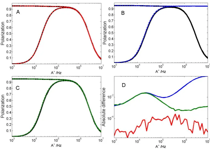
Figure 1. Simulation of the nuclear steady state polarisation for a system of one electron with one nuclear spin. The strength of the pseudosecular interactionA+ is changed between 1kHz and 10MHz. A:

Com-parison between uncorrelated random fluctuation model (10) (black) and the strategy (14) that involves the choice of the eigenbasisH00 (red).B: Comparison between random fluctuation model (10) (black) and

original Vega’s model with fluctuations only assumed alongIx (blue). C: Comparison between random fluctuation model (10) (black) and Vega’s model with fluctuations also assumed alongIz (green). D: dif-ference between the simulations. Red refers to A, blue to B and green to C. Note the logaritmic scale and the large error between simulations in C that disappears when fluctuations alongIxandIzare assumed in Vega’s model. Model parameters:ωI= 144MHz, MW= 0.1e6,R1e= 1, R2e= 1e5, r1n= 1e−2, r2n= 1e4

Figure (1) demonstrates that for the simple 2 spin systems (1e 1n) there is good agreement between the random fluctuation model Γ (10), the model-free strategy Γ0 explained in section 7 (14) and Vega’s original simulations provided that we

modify his rates in such a way that also fluctuations along Iz are allowed. This

modification of his model is essential to get good agreement with the random fluctuation model also for more than one nuclear spin.

For the case that the model spin system consists of several nuclear spins and one electron spin we demonstrate now that there could be a substantial discrepancy in the spin dynamics predictions depending on the strength of the nuclear dipolar interaction in comparison to the difference of the strength of the secular term of the hyperfine interactions of the nuclei with the electron.

We use as an example a model spin system consisting of one electron and two nuclear spins. Suppose that, calculating the basis of eigenstates of H0, we can

neglect terms, not commuting withHZ, that is we assume|Bk| |ωI|. This leads to the simplified stationary Hamiltonian

H₀0 =HZ+X

k<j dkj

2IkzIjz−

1

2Ik+Ij−− 1 2Ik−Ij+

+X

k

8.1. The case when the nuclear dipolar interaction is quenched by the hyperfine interaction - core nuclei

First we consider the case when the dipolar interaction between the nuclei is much smaller than the difference between the strength of the secular terms of the hyper-fine interaction that describes their coupling to the elctron spin. The nuclei are in this case close to the electron and the dipolar interaction between them is quenched by their coupling to the electron. In DNP models such nuclear spins belong to the core.

∀k6=j |dkj|

|Ak−Aj|1.

Under these conditions the nuclear interaction term is negligible and the basis of eigenstates ofH₀0 is well approximated by the Zeeman basis {vs}. We show in the Appendix 11.4 that in this case the two models can be modified in such a way that their predictions of the SE DNP spin dynamics are very close. Using the additional conditions that the transverse relaxation time constants are much shorter than the longitudinal time constants

1

T2e , 1

T2n,k

1

T1e , 1

T1n,k

, ∀k6=j |dkj|

|Ak−Aj|

1 (19)

the model based on the uncorrelated random fluctuations ˆΓ and the model ˆΓ0based

on the choice of the eigenbasis ofH₀0 can be made close to each other if we let ˆ

Γ0Okj =R2,kjOkj, R2,kj =T r

(ˆΓOkj)Ojk

, k6=j,

ˆ

Γ0Okk=

X

j6=k

R1,kj(Okk−Ojj), R1,kj=−T r

(ˆΓOkk)Ojj

. (20)

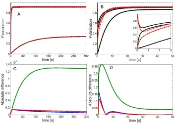
We show the good agreement for the two models (10) and (14) in Figure (2)A and C. Note that the absolute error between the two simulations is very small.

8.2. The case when the dipolar interaction is not quenched by the hyperfine interaction - the bulk nuclei

If the nuclei are relatively far away from the electron the nuclear dipolar interac-tion can be larger than the difference between the strengths of the secular hyperfine interactions of the nuclei. Such conditions can be found for bulk nuclei. The first of conditions (19) is physically reasonable and normally satisfied. The second con-dition however can be violated. In this case, the two relaxation models predict different dynamics for the spin polarisation (see Figure (2)B and D). They are inconsistent whatever rates R1,kj, R2,kj we choose. To provide more insight we

discuss in the following an instructiv example.

Let us have two nuclei and assume as before that the “effective Hamiltonian” commutes withHZ, i.e., has the form (18). Generally, there exists the unique basis, in which the both H₀0 and HZ are diagonal. In terms of Zeeman states (with the

first nucleus in the first position, the second nucleus in the second position and the electron separated with the comma), this basis is

Figure 2. Comparison between the two models (10) (red) and (14) (black). A: Time course of the po-larisation of the electron and two nuclear spins.ωI = 144MHz, MW= 0.1e6,R1e= 1, R2e= 1e5, r1n= 1e−2, r2n = 1e4,A0 = [0.155,−0.016]×1e6,A+ = [0.466,0.015]×1e6,d = 64.57 Hz. C: shows the

difference between the two simulations in A. B: All parameters are the same apart from the interaction strengthsA0= [−0.015,−0.015]×1e6,A+= [0.43,0.015]×1e6,d= 15 Hz, D: shows the difference between

the two simulations in B. The maximal absolute error is more the 30% of the spin polarisation |λ5i= cosφ+|αβ, αi+ sinφ+|βα, αi, |λ6i= cosφ+|βα, αi −sinφ+|αβ, αi,

|λ7i= cosφ−|αβ, βi+ sinφ−|βα, βi, |λ8i= cosφ−|βα, βi −sinφ−|αβ, βi,

tanφ±=±

1

d12

∆A−

q

∆2_A+d2₁₂

, ∆A=

A1−A2

2 .

The second of conditions (19) is violated when|d12| |∆|. In this case, tanφ±= ∓signd12and the following mixing of Zeeman states occurs (for d12>0)

|λ5i=

|αβ, αi − |βα, αi √

2 , |λ6i=

|βα, αi+|αβ, αi √

2 ,

|λ7i=

|αβ, βi+|βα, βi √

2 , |λ8i=

|βα, βi − |αβ, βi √

2 .

We have, for example,

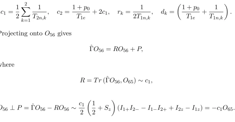
O56=

1 2

1 2 +Sz

(I1+I2−−I1−I2++I1z−I2z),

ΓO56=

1

c1 =

1 2

2

X

k=1

1

T2n,k

, c2 =

1 +p0 T1e

+ 2c1, rk=

1 2T1n,k

, dk=

1 +p0 T1e

+ 1

T1n,k

.

Projecting ontoO56 gives

ˆ

ΓO56=RO56+P,

where

R=T r(ˆΓO56, O65)∼c1,

O56⊥P = ˆΓO56−RO56∼ c1

2

1 2+Sz

(I1+I2−−I1−I2++I2z−I1z) =−c1O65.

We see that the projectionRO56and the orthogonal componentP are of the same

order ∼c1 which is the average between the transverse rates 1/T2n,1 and 1/T2n,2.

This means that the action of the relaxation superoperator ˆΓ on the non-diagonal elementO56 is strongly not proportional toO56. This will be the case for any

non-diagonal elementsOkj composed of strongly mixed Zeeman states. Using the model based on the choice of the eigenbasis of H₀0, we have always ˆΓ0Okj = R2,kjOkj, k6=j.

Thus, both models are inconsistent if the first of conditions (19) is satisfied while the second one is violated. The reason for this discrepancy is the use of the stationary Hamiltonian H0 as a reference frame for the relaxation model

(14) that is based on the choice of the eigenbasis of H₀0 and that was described in Section 7. This choice of reference frame lead for the interaction parameters used in the simulation to a violation of condition (9). To demonstrate this we provide a list of the valueskj,k0_j0 =|R_kj,k0_j0/Ω_kj,k0_j0|calculated (see formula (8)) for the simulation shown in Figure (2) in Table 1. Condition (9) which requires

kj,k0_j0 1 is not fulfilled for more than 3.6% of the 1447 non zero elements (4096 in total). Therefore, the intrinsic assumption made during the derivation of the superoperator in section 7 that non-secular terms can always be neglected in this strategy is not valid and the predictions made by model (14) will deviate from the predictions arising from the random fluctuation model (10). For the core nuclei with much stronger hyperfine interactions the values of Ωkj,k0_j0 are always bigger then the relaxation rateRkj,k0_j0 and hence there is a good agreement between the two models. This example emphasizes that particular care must be used to choose the correct interaction frame and to introduce physical meaningful relaxation mechanism.

Figure (3) provides another example of the deviations between the two models. In this case we have assumed a spin chain of 4 nuclear spins and one electron with only the first nuclear spin coupled to the electron and all other nuclear spins interacting through dipolar interaction with each other (similar to Vega’s JCP paper).

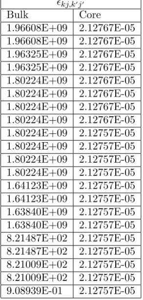
Table 1. The first representative values of_kj,k0_j0 = |R_Ωkj,k0j0 |

kj,k0j0 are provided in descending order for both the

simulation of the core nuclei and the simulation of the bulk nuclei shown in Fig.2. Note the huge deviation from

the condition_kj,k0_j01 which is required for the removal of the non-secular terms during averaging the

time-dependent relaxation superoperator (see Section 5). This provides the explanation why the model (14) which

usesH₀0 as a reference frame substantially deviates from the predictions of the uncorrelated random fluctuation

model (10). Only the first 21 value for_kj,k0j0 of the 1447 non-zero values for the core are shown. (There are

another 31 values close to 1).

kj,k0_j0

Bulk Core

1.96608E+09 2.12767E-05 1.96608E+09 2.12767E-05 1.96325E+09 2.12767E-05 1.96325E+09 2.12767E-05 1.80224E+09 2.12767E-05 1.80224E+09 2.12767E-05 1.80224E+09 2.12767E-05 1.80224E+09 2.12767E-05 1.80224E+09 2.12757E-05 1.80224E+09 2.12757E-05 1.80224E+09 2.12757E-05 1.80224E+09 2.12757E-05 1.64123E+09 2.12757E-05 1.64123E+09 2.12757E-05 1.63840E+09 2.12757E-05 1.63840E+09 2.12757E-05 8.21487E+02 2.12757E-05 8.21487E+02 2.12757E-05 8.21009E+02 2.12757E-05 8.21009E+02 2.12757E-05 9.08939E-01 2.12757E-05

a relaxation model. We can conclude that the use of H₀0 frame can lead to spin dynamic predictions that cannot be explained by spin relaxation arising from a physically reasonable fluctuation model. The relaxation model derived in section 7 (which is equivalent to the one used in Vega’s paper) can only be used for the special situation when condition (19) is satisfied.

9. Extension to more complex relaxation models

In this section we extent the discussion to more complex relaxation mechanism. Three examples are given based on the fluctuations approach described in section 5. The examples illustrate the typical mechanisms of relaxation in solids and are applicable to the electron-nuclear spin system in a SE DNP model: the electronic relaxation caused by theg-anisotropy, the nuclear relaxation caused by the electron as a paramagnetic centre and the electron-nuclear relaxation caused by vibrations of the crystalline lattice near the electronic spin.

9.1. Electron relaxation caused by g-anisotropy

The Zeeman interaction of the electronic spinSwith the static fieldB0is mediated

Figure 3. A: Polarisation dynamics in a spin chain consisting of one electron and four nuclear spins, simulated using the relaxation model (14) (red) and (10) (black). B: Difference between the predictions of the two models: blue 1st spin, green 2nd spin, red 3rd spin, light blue 4th spin, magenta electron. Note the huge difference for the prediction of the polarisation of the 3rd and 4th spin. Simulation parameters: ωI = 36MHz, MW= 0.2e6, R1e = 1e2, R2e = 1e5, r1n = 1e−2, r2n = 1e3, A0 = [0,0,0,0]×1e6,

A+= [0.04,0,0,0]×1e6,d(1,2) = 7, d(2,3) = 6, d(3,4) = 8.5Hz.

and is generally anisotropic, i.e., not represented by a simple scalar product between the vectors B0 and S. In sufficiently symmetric environment, the g-anisotropy is

relatively small, but can be appreciable in non-symmetric cases.

Considering an ensemble of electronic spins {Sk}, we have to assume that each

electron in the ensemble has its owng-tensor gk, even when the anisotropic parts of them are small. In this case,

gk=g0·1 +gk,a, kgk,ak |g0|.

Statistically the electronic ensemble is well represented by a single electron S in such way that the Zeeman interaction becomes

HZ =ωSSz+B0.ga.S, ωS=g0|B0|,

where ga is a random spatially distributed tensor. Using the ergodicity principle,

we can assume that the tensorga=ga(t) is a random function of time, interpreting

this as that anisotropies of different electron spins have different effective times, which are randomly distributed between them. An analogous assumption is made in liquid state NMR when we regard the spatially distributed ensemble molecular motion as a random temporal motion of a single molecule.

Thus, we can write

HZ =ωSSz+Hf(t), Hf(t) =fz(t)Sz+f+(t)S++f−(t)S−

with random scalar functionsfβ(t),β =z,±. We can assume thatfβ(t) are random

stationary processes with zero ensemble averages and some correlations functions

so we follow the fluctuations approach described in section 5.

The operators Sβ,β = z,± are eigenvectors of the superoperator ˆHZ with the

eigenoperator 0,±ωS respectively. This leads to the straightforward formula

ˆ

ΓS =R2Sˆz+R1

ˆ

S+Sˆ−+ ˆS−Sˆ+

(21)

with

R2=

1 2

Z +∞

−∞

gzz(τ)dτ, R1 =

1 2

Z +∞

−∞

g++(τ)eiωSτdτ =

1 2

Z +∞

−∞

g−−(τ)eiωSτdτ.

9.2. Nuclear relaxation caused by electron as paramagnetic centre

To describe the electron-nuclear hyperfine interaction in a dielectric solids between a radical centre with a locally confine electron and the surrounding nuclei we can focus mainly on the dipolar interaction and ignore the Fermi contact interaction. Taking into account the huge electronic Larmor frequencyωS in the Zeeman frame

we can write the hyperfine interaction in the reduced form

HIS =V Sz, V =

X

k

(2Ak0Ikz+Ak+Ik++Ak−Ik−).

The role of the electron as a paramagnetic centre (or impurity) is described as follows (see Bloemebrgen’s spin diffusion, Abragam-Goldman’s relaxation of II kind and others).

It is assumed that during the evolution, a spontaneous exchange occurs between the subspaces of the “up” and “down” states of the electronic spin. Due to the presence of the terms with Ik±Sz inHIS, this random process affects the nuclear

spins in the form of a random field seen by them via spontaneous changes of the sign of the coefficients Ak±. These fluctuations are seen simultaneously by

all nuclei grouped to the corresponding hyperfine interaction terms. The typical correlation time is comparable with the electronic longitudinal time T1e, so can

lead to processes with longer times thanT1e. However, this can be appreciable and

crucial for the nuclei in close electron vicinity. In terms of fluctuations, this gives

Hf(t) =f(t)V++f∗(t)V−, V±=

X

k

Ak±Ik±,

where f(t) is a random scalar function of time. We can assume again that it de-scribes a stationary process with zero average and some correlation function

f(t) = 0, g(τ) =f(t)f∗_(t−τ).

The operataors V± are eigenvectors of ˆHZ with the eigenvalues ±ωI respectively.

Using the fluctuations approach, this leads to the following superoperator

ˆ ΓI =τ0

ˆ

V+Vˆ−+ ˆV−Vˆ+

, τ0=

1 2

Z +∞

−∞

The simplest realization

g(τ) =g(−τ) = 1 4exp

−|τ|

T1e

leads to the formula

τ0=

1 4

T1e

1 +ω_I2T₁2_e ∼

1 4ω_I2

1

T1e .

It is seen that the relaxation rates are∼k/T1ewithk=|Ak±/ωI|2, so they tend

to be larger for nuclei closer to the electron and smaller for remote nuclei.

9.3. Electron-nuclear relaxation via vibrations of crystalline lattice near electron

The electron-nuclear interaction can lead to another mechanism connected with vibrations of the crystalline lattice in the electron vicinity, as follows.

Even at low temperatures, the position of the electronic spin (unlike the nuclear spins) is not fixed in space, it is found randomly in time in some volume near its average position. This causes vibrations of the crystalline lattice near the electron in the form of the phonon lattice sound. This random noise is seen by the nuclear spins via fluctuations of the coefficients of the hyperfine interaction which depend on orientations of the electron-nuclear pairs and so depend on the random electron position. In the Zeeman frame with large Larmor frequenciesωI,S, the dominating

part of the electron-nuclear interaction in the purely Zeeman part

HIS,Z = 2

X

k

Ak,0IkzSz.

The fluctuations of the coefficients Ak,0 caused by the above vibrations can be

written as

Hf(t) =X

k

fk(t)Vk, Vk= 2Ak,0IkzSz,

wherefk(t) are real scalar functions of time describing random stationary processes

with zero averages and some correlation functions

fk(t) = 0, gkj(τ) =fk(t)fj(t−τ).

The operatorsVk belong to the zero eigenspace of ˆHZ. This leads to the

superop-erator

ˆ ΓIS =

X

k,j

τkjVˆkVˆj, τkj =

1 2

Z +∞

−∞

gkj(τ)dτ. (23)

It is seen that ˆΓIS affects only non-Zeeman operators with rates proportional to Ak,0Aj,0.

Combining the models (21), (22), (23) and applying the thermalization, we obtain

˙

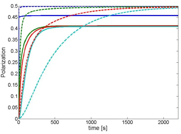
Figure 4. Comparison of the nuclear polarisation dynamics for four13_{C nuclei calculated using the simple}

uncorrelated random fluctuation model (10) (solid line) and a model taking all other mechanisms into account (broken line). Simulation parameters were MW= 0.1MHz,R1e = 1e0, R2e = 1e5, r1n = 6.5e− 4, r2n = 1e4, for the random fluctuation model andR1e = 4, R2e = 1.12e5, r1n = (6.55e−4,8.83e− 06,6.40e−07,4.13e−08), r2n = (9527,1283,930,600) for the more comprehensive model. Note that for the comprehensive model all nuclear spins reach eventually the same polarisation level

with

ˆ

Γσ= ˆΓSσ+ ˆΓIσ+ ˆΓISσ+ ˆΓth,

ˆ

Γthσ= 2p0R1(S+σS−−S−σS++Szσ+σSz).

(24)

To find connections between R1,2,τ0,τkj and the effective transverse and

longi-tudinal relaxation times, we can calculate according to (24)

ˆ

ΓSz = 4R1Sz, ΓˆS±=



R2+ 2R1+

X

k

τkk|Ak0|2+

X

k6=j

τkjAk0Aj0IkzIjz



S±,

ˆ

ΓIkz = 4τ0|Ak±|2Ikz+ 8p0R1IkzSz,

ˆ

ΓIk±= 2τ0|Ak±|2+τkk|Ak0|2

Ik±+ 8p0R1Ik±Sz,

getting effectively

1

T1e

= 4R1,

1

T2e

=R2+ 2R1+

X

k

τkk|Ak0|2,

1

T1n,k

= 4τ0|Ak±|2,

1

T2n,k

10. Conclusions and Outlook

The polarisation enhancement of the nuclear spin ensemble by solid effect DNP is the result of both the irradiation of one of the electron satellite frequencies (ωS±ωI)

and the relaxation processes in response to this preturbation. Relaxation needs to be incorporated into a quantum mechancial model to provide predictions that can be used for comparison with experimental data. We reviewed and compared several strategies and pointed out under which conditions these strategies provide predic-tions in close agreement and discussed under which condipredic-tions they fail to agree. In particular we outlined our strategy to incorporate relaxation through the as-sumption of fluctuations that modulate the interaction of the electrons and the nuclear spins with their respective environment. The mathematical advantage of our strategy is the avoidance of the diagnalisations of large matrices which enables us to increase the number of coupled nuclear spins in the quantum system. Since the dynamics of the nuclear polarisation depends on the number of coupled nu-clear spins in the spin system it is important to maximise this number in model simulations to obtain predictions close to the experimental observations.

11. Appendix

11.1. Invariance of the relaxation superoperator in the Lindblad-Kossakowski form

After proceeding to the interaction frame by the rule (4), the relaxation superop-erator (3) is transformed to

−Γˆ0¯σ=

N2₋₁ X

k=1 γk

¯

Lkσ¯L¯∗k−

1 2 ¯σL¯

∗

kL¯k+ ¯L∗kL¯kσ¯

, L¯k =ei ˆ HZt_L

k.

The Liouville space admits the following expansion into eigenspaces Vpq of the

superoperator ˆHZ (nis the number of nuclei)1

L=

n

X

p=−n 1

X

q=−1

Vpq, HZvˆ = Ωpqv, Ωpq=pωI+qωS, v∈Vpq.

Using the expansions

Lk=

X

p,q

ak,pqlk,pq, lk,pq∈Vpq, L¯k=

X

p,q

ak,pqeiΩpqtlk,pq, (25)

we obtain

¯

Lkσ¯L¯∗k−

1 2 σ¯L¯

∗

kL¯k+ ¯L∗kL¯kσ¯

=

= X

p,q,p0_,q0

ei(Ωpq−Ωp0q0)t

ak,pqa∗_k,p0_q0

lk,pqσl¯ _k,p∗ 0_q0 − 1 2 σl¯

∗

k,p0_q0lk,pq+l∗_k,p0_q0lk,pq¯σ

.

(26)

1_{We assume that the magnitudes Ωpq are all well distinguished, which is true for protons at high field.}

Effectively, the non-secular terms are averaged out, so ˆΓ0 should be time-independent. This means

ak,pqa∗k,p0_q0 = 0, (pq)6= (p0q0),

so eachLkbelongs completely to one and only one of the eigenspacesVpq, i.e., each Lk is an eigenvector of the Zeeman superoperator ˆHZ.

Thus, we conclude that the effective relaxation superoperator (3) in the inter-action frame is such that the set {Lk} of Lindblad-Kossakowski operators is an orthogonal set of traceless eigenvectors of the superoperator ˆHZ.

11.2. Derivation of the relaxation superoperator in the

Lindblad-Kossakowski form starting from a fluctuation model

We can assume that the fluctuationHf is built of a full set{Fpq,m}of orthonormal eigenoperators of ˆHZ. In the case that some eigenoperators are absent, we assign the zero value to the corresponding coefficient. Taking into account the multiplicities of eigenvalues,p∈ −n, n,q ∈ −1,1,m∈1, dim Vpq.

We have

∀m HˆZFpq,m= ΩpqFpq,m, Ωpq =pωI+qΩS,

F_pq,m0 ≡eiHˆZt_F

pq,m=eiΩp,qtFpq,m.

Hence,

H_f0(t) =X

p,q

X

m

fpq,m(t)Fpq,m0 (t) =

X

p,q

X

m

fpq,m(t)eiΩp,qtFpq,m,

ˆ

H_f0(t) ˆH_f0(t−τ) = ˆH_f0(t) ˆH_f0∗(t−τ) =

= X

p,q,p0_,q0

X

m,m0

fpq,m(t)fp∗0_q0_,m0(t−τ) exp[iΩ_pqt−iΩ_p0_q0(t−τ)] ˆF_pq,mFˆ_p∗0_q0_,m0

where ˆ over spin operators denotes the commutation superoperator of these oper-ators. Taking the ensemble average and truncating non-secular terms, we obtain

ˆ

H_f0(t) ˆH_f0(t−τ) =X

p,q

X

m,m0

cpq,mm0(τ) exp(iΩ_pqτ) ˆFpq,mFˆ∗

pq,m0,

cpq,mm0 =f_pq,m(t)f∗

pq,m0(t−τ). This leads to the general formula

ˆ Γ =X

p,q

X

m,m0

Cpq,mm0Fpq,mˆ Fˆ_pq,m∗ 0, Cpq,mm0 = 1 2

Z +∞

−∞

cpq,mm0(τ) exp(iΩpqτ)dτ.

Thermalization and reduction to Lindblad-Kossakowski form

It is seen that the form (27) is generally not in the Lindblad-Kossakowski form. The thermal correction is needed as well as the reduction of the double-commutators in a proper way. This is done as follows.

Taking Hermitian conjugate and permuting indices, we obtain

ˆ Γ =X

p,q

X

m,m0

Cpq,mm0Fpq,mˆ Fˆ∗

pq,m0 =

X

p,q

X

m,m0

C_pq,m∗ 0_mFˆ_pq,m∗ 0Fpq,m.ˆ

Since

C_pq,m∗ 0_m =C_pq,mm0,

this gives

ˆ Γ = 1

2

X

p,q

X

m,m0

Cpq,mm0

ˆ

Fpq,mFˆpq,m∗ 0+ ˆF_pq,m∗ 0Fˆ_pq,m

.

Consider the two superoperators

ˆ

U_pq,mm+ 0σ=Fpq,mσF_pq,m∗ 0− 1 2 σF

∗

pq,m0Fpq,m+F_pq,m∗ 0Fpq,mσ

,

ˆ

U_pq,mm− 0σ =F_pq,m∗ 0σFpq,m− 1

2 σFpq,mF

∗

pq,m0 +Fpq,mF_pq,m∗ 0σ

and rewrite ˆΓ as

−Γˆ0 =X

p,q

X

m,m0

Cpq,mm0

ˆ

U_pq,mm+ 0+ ˆU_pq,mm− 0

+X

p,q

X

m,m0

C_pq,mm− 0

ˆ

U_pq,mm+ 0−Uˆ_pq,mm− 0

.

In accordance with the formula

ˆ

Fpq,mFˆpq,m∗ 0+ ˆF_pq,m∗ 0Fˆ_pq,m=−2

ˆ

U_pq,mm+ 0+ ˆU_pq,mm− 0

,

the superoperator ˆΓ0 is in the Lindblad-Kossakowski form and coincides with ˆΓ for

C_pq,mm− 0 = 0. We can choose C_pq,mm− 0 in such way that

ˆ

Γ0σth= 0.

Then the master equation

˙

σ=−iHˆ0σ−Γˆ0σ

is the needed homogeneous Lindblad-Kossakowski form where the full density op-erator should be used. Here we can apply the approximation

σth=

1

N (1−2p0Sz), p0= tanh

~ΩS

11.3. Derivation of the relaxation superoperator based on the uncorrelated random fluctuation model

Let us introduce the superoperators

ˆ

Uzσ =SzσSz−1

2(σSzSz+SzSzσ), ˆ

U±σ =S±σS∓−1

2(σS∓S±+S∓S±σ),

ˆ

ukzσ=IkzσIkz−1

2(σIkzIkz+IkzIkzσ), ukˆ ±σ=Ik±σIk∓− 1

2(σIk∓Ik±+Ik∓Ik±σ)

and the commutation superoperators

ˆ

L≡[L,·], L=Sz, S±, Isz, Is±.

Due to the relations valid for any spin 1/2

I_z2 = 1

4, I±I∓= 1 2±Iz,

we have

ˆ

Uz =−1

2 ˆ

S_z2, ukzˆ =−1

2 ˆ

I_kz2 ,

ˆ

U++ ˆU−=−

1 2

ˆ

S+Sˆ−+ ˆS−Sˆ+

, ukˆ ++ ˆuk−=−

1 2

ˆ

Ik+Ikˆ−+ ˆIk−Ikˆ+

,

( ˆU+−Uˆ−)σ =S+σS−−S−σS++σSz+Szσ,

(ˆuk+−uˆk−)σ =Ik+σIk−−Ik−σIk++σIkz+Ikzσ.

This gives

ˆ

Γσ=R2Sˆz2σ+R1

ˆ

S+Sˆ−+ ˆS−Sˆ+

σ+R3(S+σS−−S−σS++σSz+Szσ) +

+

n

X

k=1

h

r2kIˆkz2 σ+r1k

ˆ

Ik+Iˆk−+ ˆIk−Iˆk+

σ+r3k(Ik+σIk−−Ik−σIk++σIkz+Ikzσ)

i

(28) whereRj,rjk are some rates to be specified.

11.4. Comparison of the action of the two models Γ0 and Γ for core nuclei

In this basis, each non-diagonal elementOkj =vkvj∗,k 6=j, is represented by one

of the following forms

Okj =SβOZ m

Y

s=1

Isβs, Okj =

1 2±Sz

OZ m

Y

s=1

where OZ is a combination of Zeeman orders built of spins other than S, Is. For

example (the electronic state is separated with the comma),

|αβ, αihββ, β|=S+I1+

1 2 −I2z

, |αβ, αihββ, α|=

1 2 +Sz

I1+

1 2−I2z

.

Since T2e, T2n,k T1e, T1n,k, the acton of our relaxation superoperator ˆΓ on Okj

in the first case is well approximated as

ˆ

ΓOkj =R02,kjOkj, R20,kj=

1

T2e

+

m

X

s=1

1

T2n,s .

In the second case,

ˆ ΓOkj ∼

1 2 m X s=1 1

T2n,s

!

OZYIsβs+

p0±1 T1e

±

m

X

s=1

1

T2n,s

!

OZSzYIsβs

which leads to the approximation

ˆ

ΓOkj =R002,kjOkj, R200,kj= m

X

s=1

1

T2n,s .

This means that the result of action of ˆΓ on Okj is approximately proportional to Okj. Hence, in the model ˆΓ0, we should let

ˆ

Γ0Okj =R2,kjOkj, R2,kj =T r

(ˆΓOkj)Ojk

.

In this case, the “transverse parts” of the both relaxation superoperators will be close.

Each diagonal element is represented as

Okk=

1 2+βSz

n

Y

s=1

1

2 +βsIsz

, β, βs=±.

For example,

|αβ, αihαβ, α|=

1 2 +Sz

1 2+I1z

1 2 −I2z

.

The action of the relaxation superoperator ˆΓ onOkkgives a traceless combination of

Zeeman orders. Any such combination is expanded into a combination of operators

Okk−Ojj exactly as in the model ˆΓ0. Hence, we should choose

ˆ

Γ0Okk=

X

j6=k

R1,kj(Okk−Ojj), R1,kj =−T r

(ˆΓOkk)Ojj

11.5. Numerical implementation of the Lindblad-Kossakowski relaxation superoperator form

In this section we recapitulate some of the information already presented in sec-tion 7 and 8 and explain how the Linbland-Kossakowski form of the relaxasec-tion superoperator for the model free approach (14) can be conveniently calculated. The Linbland-Kossakowski form of the relaxation superoperator is given by (14):

−Γˆ0σ=

X

s6=s0 Γss0

Oss0σO_s0_s− 1

2(σOs0s0+Os0s0σ)

+ +X q Γq

OqσOq−

1

2(σOqOq+OqOqσ)

.

Where ˆΓ0 indicates a matrix of the relaxation superoperator for the model-free

approach,Oss0 =vsv∗_s are the eigenoperators constructed from the eigenvectors of the stationary Hamiltonian in the Hilbert space. The requirement that the oper-ators Oss are traceless can be fulfilled by setting up a linear combination of the former: Oq =PNs=1cqsOss . The coefficientcqs are found by solving a set of

equa-tions given in (15). To avoid these cumbersome calculaequa-tions we can further simplify (14), the second term can be rewritten in the non-diagonal form:

X

q0 Γq

OqσOq−

1

2(σOq+Oqσ)

=

X

ss0 ¯ Γss0

OssσOs0_s0 − 1

2(σOs0s0Oss+Os0s0Ossσ)

=

X

s6=s0 ¯

Γss0O_ssσO_s0_s0+

X

s

¯ Γss

OssσOss−1

2(σOss+Ossσ)

(29)

where the rates ¯Γss0 are expressed via Γ_q and cqs. It follows from the form of (14) that:

ˆ

Γ0Okk=

X

s6=k

R1,sk(Okk−Oss), Γˆ0Okj =R2,kjOkj, k6=j,

which in terms of the rates ¯Γss0’ and gives us:

R2,kj =

1 2



Γ¯kk+ ¯Γjj−2¯Γkj+

X

s6=k

Γsk+

X

s6=j

Γsj



, R1,sk = Γsk (30)

If the ratesR1,sk, R2,kj are known one can invert the relation in (30) to find ¯Γss0 and Γss0, letting further ¯Γ_ss0 = 0 one gets:

Γsk =R1,sk, Γ¯kj =

1 2



 X

s6=k

R1,sk+

X

s6=j R1,sj



The ratesR1,sk,R2,kj can be found from the projection of the eigenoperators Okj: R2,kj =T r

h

ˆ ΓOkj

Ojk

i

, R1,sj=−T r

h

ˆ ΓOkk

Oss

i

, (32)

where ˆΓ is the relaxation superoperator matrix for the uncorrelated random field model given by (10). To calculate the projection, operatorsOkjhave be represented

column wise as vectors. The trace is taken if the product of ˆΓOkj is transform back

the operator representation or the scalar product ifOjkis in the vector form. Finally the following expression for the relaxation superoperator matrix of the model-free approach is obtained:

−Γˆ0σ=

X

s6=s0 Γss0

Oss0σO_s0_s− 1

2(σOs0s0+Os0s0σ)

+

+X

s6=s0 ¯

Γss0OssσOs0_s0

(33)

The advantage of the form (33) is that it contains only the operators Oss0 and rates Γss0, ¯Γ_ss0 easily calculated from (31) and (32).This form is especially conve-nient if operatorsOss0 are expressed as the left/right superoperators (operators in Liouville space) i.e. ˆOL_ss0 =Oss0⊗1, ˆOR