Astronomy & Astrophysicsmanuscript no. 13723˙referee c ESO 2010 February 3, 2010
Three-Dimensional Solutions of the
Magnetohydrostatic Equations: Rigidly Rotating
Magnetized Coronae in Cylindrical Geometry
Nasser Al-Salti
⋆, Thomas Neukirch, and Richard Ryan
School of Mathematics and Statistics, University of St. Andrews, St. Andrews KY16 9SS, United
Kingdom
Received/Accepted
ABSTRACT
Context.Solutions of the magnetohydrostatic (MHS) equations are very important for modelling
astrophysical plasmas, for example the coronae of magnetized stars. Realistic models should be
three-dimensional, i.e. should not have any spatial symmetries, but finding three-dimensional
so-lutions of the MHS equations is a formidable task. Only very few analytic soso-lutions are know and
even calculating solutions with numerical methods is usually far from easy.
Aims.We present a general theoretical framework for calculating three-dimensional MHS
solu-tions outside massive rigidly rotating central bodies, together with example solusolu-tions. A possible
future application is to model the closed field region of the coronae of fast rotating stars.
Methods.As a first step, we present in this paper the theory and solutions for the case of a massive
rigidly rotating magnetized cylinder, but the theory can easily be extended to other geometries,
We assume that the solutions are stationary in the co-rotating frame of reference. To simplify
the MHS equations, we use a special form for the current density which leads to a single linear
partial differential equation for a pseudo-potential U. The magnetic field can be derived from U
by differentiation. The plasma density, pressure and temperature are also part of the solution.
Results.We derive the fundamental equation for the pseudo-potential both in coordinate
inde-pendent form and in cylindrical coordinates. We present numerical example solutions for the case
of cylindrical coordinates.
Key words. Magnetic fields - Magnetohydrodynamics (MHD) - Stars: magnetic fields - Stars:
coronae - Stars: activity
1. Introduction
Finding three-dimensional (3D) solutions of the magnetohydrostatic (MHS) equations, i.e. solu-tions with no spatial symmetry, is a formidable task. Only very few analytical solusolu-tions are known and even using numerical methods for calculating 3D MHS solutions is usually far from straight-forward (e.g Wiegelmann & Neukirch 2006; Wiegelmann et al. 2007).
⋆ Permanent address: DOMAS, Sultan Qaboos University, P.O. Box 36 P.C. 123 Muscat, OMAN. E-mail:
Analytic solutions have been found for a number of different cases.1If external forces like the gravitational force or the centrifugal force can be neglected, force balance between the Lorentz force and the pressure gradient has to be achieved. A small number of analytical solutions in Cartesian and cylindrical coordinates have been found (e.g Woolley 1976, 1977; Shivamoggi 1986; Kaiser et al. 1995; Salat & Kaiser 1995; Kaiser & Salat 1996, 1997) and some of them have been generalized to include field-aligned incompressible flows (Petrie & Neukirch 1999).
The case where external forces cannot be neglected is often the more relevant for astrophysical applications. In particular, three-dimensional solutions of the MHS equations in the presence of an external gravitational field have been found for this case, both in Cartesian (e.g. Low 1982, 1984, 1985, 1992, 1993a,b; Neukirch 1997; Neukirch & Rast¨atter 1999; Petrie & Neukirch 2000) and in spherical coordinates (e.g. Osherovich 1985a,b; Bogdan & Low 1986; Neukirch 1995).
For the case of the presence of external forces, a systematic method for calculating a special class of 3D MHS equilibria has been developed in a series of papers by Low (1985), Bogdan & Low (1986), Low (1991), Low (1992), Low (1993a), Low (1993b) and Low (2005). The method is applicable to all external forces derived from a potential and assumes a special form for the electric current density to allow analytical progress. In the simplest possible case, the MHS equa-tions reduce to a linear partial differential equation for the magnetic field. It has been shown that in Cartesian and spherical geometry, the fundamental equation is very similar to a Schr¨odinger equa-tion (Neukirch 1995; Neukirch & Rast¨atter 1999). Therefore standard methods such as expansion in terms of orthogonal function systems (e.g. Rudenko 2001) or Green’s functions (e.g. Petrie & Neukirch 2000) can be used for finding solutions, and this method has been used to model, for example, the solar corona (e.g. Zhao & Hoeksema 1993, 1994; Gibson & Bagenal 1995; Gibson et al. 1996; Zhao et al. 2000; Ruan et al. 2008) and stellar coronae (e.g. Lanza 2008).
While the method has been mainly used to find 3D MHS solutions for the case of an external gravitational potential, Low (1991) has also developed the method for rigidly rotating systems sub-ject to centrifugal forces. For those cases the system is stationary only in the frame of reference rotating with the same angular velocity as the system itself. Recently, Neukirch (2009) has pre-sented a couple of 3D MHS solutions for rigidly rotating magnetospheres in cylindrical geometry, again using the simplest case leading to a linear differential equation for the magnetic field.
In the present contribution we extend the theory to the case where both gravitational and cen-trifugal force are taken into account. This case is, for example, relevant for the coronal structure of fast rotating stars (e.g. Jardine & Unruh 1999; Jardine 2004; Jardine & van Ballegooijen 2005; Ryan et al. 2005; Townsend & Owocki 2005; Townsend et al. 2005; ud-Doula et al. 2006), in partic-ular for the closed field line region. Often, however, potential magnetic fields are used for models derived from stellar surface data (e.g. Jardine et al. 1999, 2001, 2002; Donati et al. 2006, 2008; Morin et al. 2008), while there is observational evidence for the non-potentiality of some measured surface magnetic fields (e.g. Hussain et al. 2002). Recently, Mackay & van Ballegooijen (2006) and Yeates et al. (2008) developed a numerical technique to produce sequences of quasi-static non-linear force-free equilibria from time series of observed magnetograms. While this technique was so far only applied to the Sun, it could in principle also be applied to other stars if magnetic field data with a sufficiently high time cadence are obtained. The theory presented in this paper could
Al-Salti et al.: 3D MHS Solutions of Rotating Magnetized Coronae 3
prove the potential field models and, in its simplest form, is not computationally more demanding than potential field models.
As in Neukirch (2009), we will present the theory in a general form following Low (1991), but then investigate the somewhat artificial, but illustrative case of a massive rigidly rotating central cylinder. This is done merely for mathematical convenience as it is much easier to impose boundary conditions on a cylindrical boundary. A full solution of the problem would also include a stellar wind on open field line regions and the need to solve a free boundary problem to determine the transition from open to closed field regions. A solution to this problem is beyond the scope of the present paper and we neglect flows altogether. Instead, for the solutions presented in this paper, we impose boundary conditions on an imaginary outer boundary, similar to the source surface used for potential field models. For this case, we determine solutions using standard numerical methods. In future work, one could as a first step towards solving the full problem, assume that the open field line regions are potential and thus try to determine the boundary between open and closed field line regions.
The paper is organized as follows. In Sect. 2 we present a brief derivation of the underlying theory, followed by illustrative example solutions in Sect. 3. We conclude the paper with a summary and discussion in Sect. 4.
2. Theory
2.1. Coordinate-Independent Theory
Before moving on to the special case of a massive rigidly rotating cylinder, we briefly outline the basic theory in a coordinate-independent form. In this way, the equations derived below are applicable to other cases as well, such as massive rigidly rotating spheres or ellipsoids (stars), or even synchronously rotating double stars, using e.g. the Roche potential.
We basically follow Low (1991) in our outline and refer the reader to his paper for more details (see also Neukirch 2009). The MHS equations in the co-rotating frame of reference are given by (see e.g. Mestel 1999))
j×B− ∇p−ρ∇V = 0, (1)
∇ ×B = µ0j, (2)
∇ ·B = 0, (3)
where B is the magnetic field, j is the current density, p is the pressure,ρis the plasma density and V is the combined centrifugal and gravitational potential. Assuming
µ0j=∇F× ∇V, (4)
with F a free function one finds from the force balance equation (1) that
p(̟, φ,z)=p(F,V), (5)
and ∂p ∂F !
V
= −1
µ0
(B· ∇V), (6)
ρ = − ∂p ∂V !
F
+ 1
µ0
Further progress can be made by making an appropriate choice for the free function F. Choosing
F(̟, φ,z)=κ(V)B· ∇V, (8)
withκ(V) a free function, as suggested by Low (1991), leads to a linear relation between magnetic field and current density. In this case, we have the following expression
p=p0(V)− 1 2µ0
κ(V)(B· ∇V)2 (9)
for the pressure. Here, p0(V) is an arbitrary function which represents a hydrostatic background atmosphere. For the density we find
ρ=−dp0 dV +
1 2µ0
dκ
dV (B· ∇V) 2+ 1
µ0
κ(V)B· ∇(B· ∇V). (10)
An expression for the plasma temperature can be obtained if we assume that the plasma satisfies the equation of state of an ideal gas,
T = µp
Rρ, (11)
where R is the universal gas constant andµis the mean molecular weight. By integrating Amp`ere’s law (2) one finds the magnetic field to be
B=∇U+ κ(V)
1−κ(V)(∇V)2(∇U· ∇V)∇V. (12)
where the free function U appears due to the integration. The pseudo-potential U is determined by substituting (12) into∇ ·B=0 :
∇ · ∇U+ κ(V)
1−κ(V)(∇V)2(∇U· ∇V)∇V !
=0. (13)
Equation (13) is a single partial differential equation for the pseudo-potential U and is the funda-mental equation for the linear case of the theory presented here. An alternative form of this equation is
∇ ·(M· ∇U)=0, (14)
with the 3×3 matrix M defined as
M=I+ κ(V)
1−κ(V)(∇V)2∇V∇V. (15)
Here I is the 3×3 unit matrix. Equation (14) is particularly useful if∇V has more than one non-vanishing component. This would, for example, be the case for the combined gravitational and centrifugal potential outside a massive rigidly rotating sphere. In such a case, Eq. (13) is usually not separable.
2.2. Cylindrical Geometry
To illustrate how the theory presented above can be used, we treat in the present paper the somewhat artificial, but mathematically simpler case of a cylinder of radius R, infinite length and uniform mass per unit length M, rotating rigidly with angular velocityΩabout its symmetry axis. We use a co-rotating cylindrical coordinate system̟,φ, z with the z-axis aligned with the rotation axis. The external gravitational potential (normalized to 0 at̟=R) of such a cylinder is given by
Al-Salti et al.: 3D MHS Solutions of Rotating Magnetized Coronae 5
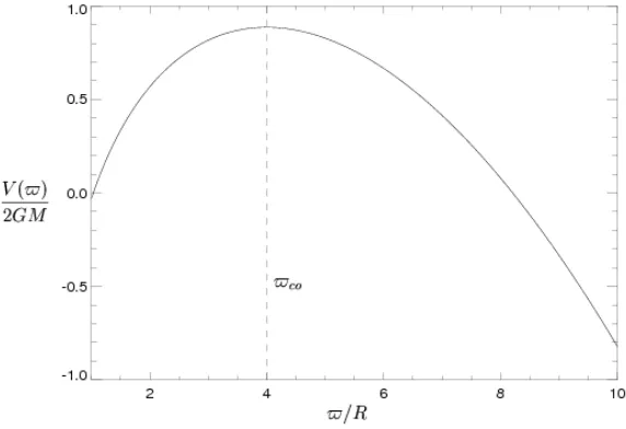
Fig. 1. The combined potential V(̟) for a co-rotation radius̟co=4.0.
and the combined potential V by
V =−Ω 2
2 ̟
2+2GM ln(̟/R). (17)
Using Eq. (12), the components of B in cylindrical coordinates are
B̟ =
1 1−κ(V)(V′)2
∂U
∂̟, (18)
Bφ =
1 ̟
∂U
∂φ, (19)
Bz = ∂U
∂z, (20)
with
V′= dV
d̟. (21)
Defining
ξ(̟)=κ(V)(V′)2, (22)
one can rewrite Equation (13) as 1
̟ ∂ ∂̟
̟ 1−ξ(̟)
∂U ∂̟
!
+ 1
̟2
∂2U
∂φ2 +
∂2U
∂z2 =0, (23)
which is the fundamental equation to be solved. The pressure and density are given by
p=p0(V)− 1 2µ0
κ(V)V′2B2̟ (24)
and
ρ=−dp0 dV +
1 2µ0
dκ dVV
′2 B2̟+ 1
µ0
κ(V) V′′B2̟+ 1 µ0
κ(V) V′B· ∇B̟. (25)
not have a one-to-one mapping to the radial coordinate̟ as the gravitational potential or the centrifugal potential on their own have. Instead, V(̟) has a maximum (see Figure 1) at the co-rotation radius given by
̟co=
√ 2GM
|Ω| . (26)
A test particle in a circular and planar orbit around the cylinder would have an orbital angular velocity which is equal toΩso that it would co-rotate with the cylinder. More importantly, though, for a rigidly rotating plasma on the cylindrical surface with radius equalling the co-rotation radius, the outward centrifugal force is exactly balancing the inward gravitational force, as the expression
−ρ∇V =−ρV′e̟
for the combination of the two forces shows. Since V′vanishes at̟co, the combined force is zero
for̟=̟co. For distances from the cylinder larger than the co-rotation radius the centrifugal force will be bigger than the gravitational force (V′ < 0) and thus the combined force will be
point-ing outward. Obviously, overall force balance will have to include the Lorentz force and pressure gradient. The Lorentz force is crucial to be able to obtain force balance beyond the co-rotation radius.
In Neukirch (2009) the expressionκ(V)V′2was generally replaced by a functionξ(̟). Due to the one-to-one mapping between the centrifugal potential and the radial variable̟, it was possible to choose the functionξ(̟) instead ofκ(V). This is not generally possible for the combined poten-tial discussed here. Although defining a functionξ(̟) =κ(V)V′2 is of course possible, choosing ξ(̟) instead ofκ(V) will generally lead to problems, for example to possible singularities ofκ(V) at the co-rotation radius, because
κ(V(̟))= ξ(̟)
V′2(̟). (27)
Obviously the denominator vanishes at̟coandκ(V) will only be non-singular ifξ(̟) goes to zero with the same or a higher power of̟−̟co at the co-rotation radius. This excludes any simple choice such asξ(̟)=ξ0=constant, which was one of the examples used in Neukirch (2009).
Singularities in κ(V) in turn lead to singularities of density and temperature as well. If we express the density in terms ofξ(̟) instead ofκ(V) we first obtain
ρ=−dp0 dV +
1 2µ0
dκ dVV
′2 B2̟+ 1
µ0
κ(V) V′′B2̟+ 1 µ0
κ(V) V′B· ∇B̟. (28)
Using dξ d̟ =
d d̟
κ(V)V′2
= dκ dVV
′3
+2κ(V)V′V′′,
we can rewrite Equation (28) in the form
ρ=−dp0 dV +
1 V′
1 2µ0
dξ d̟B
2 ̟+ 1 V′ 1 µ0
ξ(̟)(B· ∇B̟), (29)
which makes the possible singularity at̟ =̟co(V′ =0) obvious. The pressure is always non-singular since
p=p0(V)− 1 2µ0
κ(V)V′2B2̟=p0(V)− 1 2µ0
Al-Salti et al.: 3D MHS Solutions of Rotating Magnetized Coronae 7
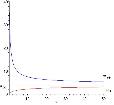
Fig. 2. The critical points̟2
s+(blue) and̟2s−(red) for a co-rotation radius̟co=2.0.
But even if a singularity ofκ(V) andρcould be avoided for a suitable choice ofξ(̟) (going through 0 quadratically at̟co), the inverse mapping from̟to V would not be well-defined across ̟co, and therefore a given functionξ(̟)/V′2(̟) cannot generally be expressed as a function of V. This has to borne in mind when we considering Eq. (23) in whichξ(̟) should merely be regarded as an abbreviation forκ(V)V′2, but not as an independent free function as, for example, in Neukirch (2009).
As already stated above, Eq. (23) is the fundamental equation that has to be solved. It is straight-forward to see that for
1−κ(V)V′2=1−ξ(̟)≷0, (31)
Eq. (23) is either elliptic or hyperbolic, respectively, while having singularities at any radius̟s whereκ(V)V′2 =1. Obviously, none of the singularities coincides with the co-rotation radius (at
̟ = ̟co we have 1−κ(V)V′2 = 1). The singularities, i.e. the transition from an elliptic to a hyperbolic equation or vice versa can only occur for κ(V) positive. For example, assuming for simplicity thatκ >0 is constant, the critical points occur at
̟2s
±=
̟2
co 2
̟2co
(2GM)2κ +2 !
±
s
̟2
co (2GM)2κ +2
!2
−4
. (32)
The critical point defined by̟2s+is beyond the co-rotation radius, whereas the one given by̟
2
s−is within the co-rotation radius (see Fig. (2). The inner singularity lies inside the central cylinder, if
(2GM)2κ < ̟
4
coR
2
(̟2
co−R2)2 ,
where of course R2 < ̟2co. One should note, however, that Eq. (32) only applies ifκ =constant. Ifκdepends on V (and thus on̟), even the possibility of more than two critical points exists in principle.
κ=0 (potential field) and then slowly increasesκshows that the radial component of the magnetic field will increase due to the decrease of 1−κV′2, if one assumes that to lowest order U does not change too rapidly with changingκ. Furthermore it is relatively straightforward to see that the radial component of the Lorentz force will be directed inwards for magnetic fields which have the same general behaviour as a dipole field close to the equator (z=0). This is exactly what is expected of stretched magnetic fields acting to confine plasma pulled away from the cylinder by the centrifugal force.
In this paper we will only consider Eq. (23) for cases where it is elliptic. We shall follow a common approach used in solar and stellar applications and in addition to the inner cylindrical boundary define an artificial outer boundary. This is similar to the source surface used in many global potential magnetic field models of the solar corona (the so-called potential field source surface or PFSS models). It should be noted, however, that because the magnetic fields calculated in the present paper are non-potential, we impose slightly different boundary conditions from those usually imposed on a source surface when potential fields are used.
3. Solution Methods and Example Solutions
In this section we discuss possible solution methods and a few illustrative example solutions. We first nondimensionalise all quantities and equations usinge∇ = R∇,̟e = ̟R,eB = BB
0,eV = V
2GM, ej= (B j
0/µ0R),ep= p B2
0/µ0, andeρ= ρ
B2
0/(2µ0GM), where B0is a typical magnetic field value. The
dimen-sionless combined centrifugal and gravitational potential is given by
V =− 1 2̟2
co
(̟2−̟2coln(̟2)), (33)
where, ̟co =
√
2GM/|Ω|
R is the dimensionless co-rotation radius and the cylinder radius in these dimensionless coordinates is 1 .
3.1. Separation of Variables
In the case when it is elliptic, Eq. (23) is very similar to Laplace’s equation and admits separable solutions (see also Neukirch 2009) of the form
U(̟, φ,z)=Fmk(̟) exp(imφ) exp(ikz). (34)
If we substitute (34) into (23) we find that the radial function Fmk(̟) satisfies the equation 1
̟ d d̟
̟ 1−ξ(̟)
dFmk d̟
!
− m
2
̟2 +k 2
!
Fmk=0. (35)
This ordinary second order differential equation will have two linearly independent solutions, Fmk(1)(̟) and Fmk(2)(̟), say. Since the partial differential equation for U is linear, the solutions for different m and k may be superposed to generate other solutions, and the most general form of a solution of (23) is
U(̟, φ,z)=
∞
X
m=−∞
exp(imφ) Z ∞
−∞
dk[Am(k)Fmk(1)(̟)+Bm(k)Fmk(2)(̟)] exp(ikz). (36)
Al-Salti et al.: 3D MHS Solutions of Rotating Magnetized Coronae 9
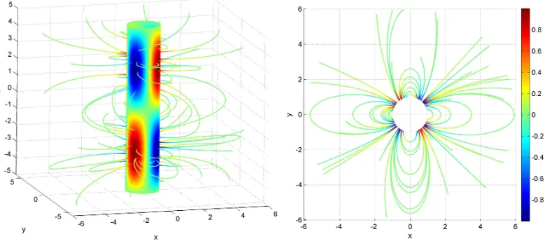
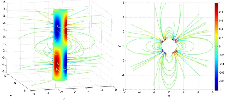
Fig. 3. Field line plots for the example solution. The left panel shows a side view, the right panel a view along
the z-axis. The colours on the boundary represent the radial magnetic field component, B̟on that boundary.
As already discussed above, we are not allowed to choose the functionξ(̟) in the present case, if the domain includes the co-rotation radius. However, to illustrate the method and for use as a test case for the numerical method used later, we show a few plots for an analytical solution which can be obtained forξ(̟)=ξ0 =constant (see e.g. Neukirch 2009). In this case the general solutions to Eq. (35) are given by
Fmk(̟)=Am(k) Iν(k
p
1−ξ0 ̟)+Bm(k) Kν(k
p
1−ξ0̟), (37)
where Iν(x) and Kν(x) are modified Bessel functions (Abramowitz & Stegun 1965),ν=m
p 1−ξ0. Am(k) and Bm(k) are constants which would usually be determined by the boundary conditions.
For this illustrative example we have chosen the parameter valuesξ0=3/4, m=2 and k=π/5,. This choice of parameters leads to p1−ξ0 = 1/2 andν = m
p
1−ξ0 =1, and we set Am(k) = Bm(k)=0, except for B±2(k) which we choose so that the pseudo-potential is given by
U=B0K1(π ̟/10) sin(2φ) sin(πz/5). (38)
The magnetic field components are then given by B̟ = −
2π
5 B0[K0(π ̟/10)+ 10
π ̟K1(π ̟/10)] sin(2φ) sin(πz/5), Bφ =
2 B0
̟ K1(π ̟/10) cos(2φ) sin(πz/5), (39)
Bz = πB0
5 K1(π ̟/10) sin(2φ) cos(πz/5).
The reason we choose Kνinstead of Iνis that Kνdecreases with increasing argument, which means
that the magnetic field strength decreases with increasing distance from the z-axis. In Fig. 3 we show a three-dimensional plot of magnetic field lines from two different viewing angles. The boundary colours represent the radial magnetic field component, B̟. The non-symmetric nature
of the magnetic field is obvious from the plot. The pressure is given by p=p0(V)−
ξ0 2B
2
̟=p0(V)− 3 4B
2
̟, (40)
which as discussed above is non-singular at the co-rotation radius. The density, however, is given by
ρ=−d p0 dV +
ξ0
V′B· ∇B̟=−
d p0 dV +
3̟2
co̟ 4(̟2
co−̟2)
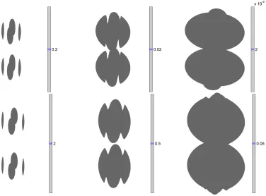
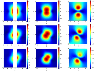
Fig. 4. Cross section plots of the pressure (top panels) and density (bottom panels) variations in the xz−plane
at y=0.5, y=1, and y=2.5, respectively.
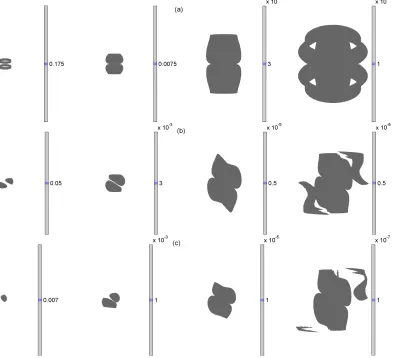
Fig. 5. Examples of pressure (top panels) and density isosurfaces (bottom panels).
and here the singularity at the co-rotation radius̟cois obvious. We therefore consider this solution only for̟ < ̟co. It should be noted that whenξ(̟) is chosen directly, the value of the co-rotation radius affects the solution only through the presence of V′in the density. As the co-rotation radius is
[image:10.595.50.426.315.593.2]Al-Salti et al.: 3D MHS Solutions of Rotating Magnetized Coronae 11
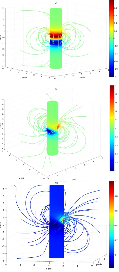
Fig. 6. 3D file line plot (left panel) and a view along the z-axis (right) for the numerical solution of the
ξ(̟)=ξ0=3/4 case. The similarity of the plots with Fig. 3 is obvious.
pressure and density contours and isosurfaces are shown in Figs. 4 and 5. Note that in the plots we only show the deviations from the cylindrically symmetrical background pressure and density.
3.1.1. Numerical Solutions of Eq. (23)
In general, finding analytical solutions of Eqs. (23) or (35) will be impossible even for simple choices of the functionκ(V). Thus, numerical methods will have to be used to find solutions. Since Eq. (23) is a simple linear partial differential equation, standard numerical methods can be used to solve it. In the present paper we used an adaptive mesh finite element method from the COMSOL Multiphysics 3.4 package with MATLAB to solve Eq. (23).
To check the accuracy of our numerical method, we have first solved Eq. (23) for the constant ξ case presented in Sect. 3.1, using the same parameter values, as well as boundary conditions that are consistent with the analytical solution. We solve Eq. (23) for U on a numerical domain, which is bounded by an inner cylinder of radius 1, an outer cylinder of radius̟o =6, and which extends from−5 to 5 in the z-direction. The outer boundary̟ois assumed to be smaller than the co-rotation radius in this case to avoid singularities in the density.
The exact boundary conditions used for this case are
– B̟(1, φ,z)=B̟,analytical(1, φ,z) on the inner boundary, where B̟,analytical(̟, φ,z) is the expres-sion given in (39),
– U(6, φ,z) =Uanalytical(6, φ,z) on the outer boundary, where Uanalytical(̟, φ,z) is given by Eq. (38) and
– n·B=0 at z=±5.
The mesh size used for this calculation consists of 261996 elements.
[image:11.595.45.435.57.231.2]Having thus convinced ourselves that the numerical tool gives satisfactory results, we have considered the simplest possible choice ofκ(V), which is
κ(V)=κ0 =constant (42)
as an example for a case whereκis chosen directly. We have calculated numerical solutions to Eq. (23) using as boundary conditions on the surface of the central cylinder (̟=1) a magnetic dipole field (Bdip) for the three cases of the
(a) magnetic dipole moment at the origin and aligned with the rotation axis (aligned rotator), (b) magnetic dipole moment at the origin, but inclined with respect to the rotation axis (oblique
rotator) and
(c) magnetic dipole moment not located at the origin and inclined with respect to the rotation axis (displaced dipole).
These three cases are similar to the cases discussed by Neukirch (2009).
We use the same domain and mesh size as in the previous example, with the outer boundary conditions given by U(6, φ,z)=Uo(6, φ,z), where U(̟, φ,z) satisfies∇Uo=Bdipand n·B=0 at z=±5.
By choosingκ(V), the density remains non-singular at the co-rotation radius. Hence, we can now calculate solutions in a domain including and extending beyond the co-rotation radius.
Numerical solutions for the case ofκ = 34 and̟co =3.5 are illustrated in Figures (7) - (10), where the letters (a), (b) and (c) above each plot indicate the three different boundary conditions mentioned above. For the oblique rotator case the magnetic dipole moment is in the x-z-plane at an angle of π4 with the x-axis. For the displaced dipole case the magnetic moment is again in the x-z-plane, but now at x=0.3, making an angle ofπ4 with the x-axis. In the plots showing pressure and density, we only show the three-dimensional deviation from background pressure and density. It turns out that both the three-dimensional pressure deviation and the three-dimensional density deviation are negative, which means that these terms will reduce any background pressure and density to lower values.
Figure (7) shows magnetic field line plots, with the colour contours on the central cylinder in-dicating the strength of the radial magnetic field component, B̟, for the three different boundary
conditions. As is to be expected, the change of boundary conditions has a clear effect on the struc-ture of the magnetic field, which is clearly symmetric for the aligned rotator case, but becomes non-symmetric for the other two cases.
This is also visible in Fig. (8), where we show isosurfaces of the three-dimensional deviation of the pressure from the background pressure. One can see that one has smaller isosurfaces close to the inner boundary where the magnetic field (and thus the pressure deviation) is strong, whereas the isosurfaces become more extended as one moves away from the cylinder and the magnetic field becomes weaker.
Al-Salti et al.: 3D MHS Solutions of Rotating Magnetized Coronae 13
Fig. 7. Magnetic field lines plots for the three cases of (a) aligned rotator, (b) oblique rotator and (c) displaced
dipole.
Figures (9) and (10) show cross section plots of the variation of the 3D pressure and density deviations from the background pressure and density in planes parallel to the xz-plane for different y-values. These plots show that there is some symmetry of the pressure and density deviations
Fig. 8. Pressure isosurface plots for the aligned rotator case (top panels), the oblique rotator case (middle
panels) and the displaced dipole case (bottom panels). The transition from rotational symmetric isosurfaces in
the aligned rotator case to asymmetric isosurfaces in the other two case can be seen very clearly.
plots. In the rightmost panels, the plane basically touches the co-rotation cylinder and thus one only sees a single broad vertical feature. It can be easily seen (e.g. from Eq. (24)) that the total pressure is equal to the background pressure at the co-rotation radius, i.e p=p0(V) at̟ =̟co. The dark vertical features in Fig. (9) thus correspond to a vanishing three-dimensional pressure deviation, whereas no corresponding feature exists for the three-dimensional density deviation (Fig. 10). The pressure and density cross-section plots confirm the increasing degree of asymmetry when going from the aligned rotator case over the oblique rotator case to the displace dipole moment case.
4. Summary and Discussion
We have presented a relatively simple (semi-)analytical approach which allows the modeling of three-dimensional rigidly rotating magnetized coronae or magnetospheres around massive central objects. In the present paper we have restricted our analysis for illustrative purposes to the simpler, but less realistic case of cylindrical geometry. The possibility of extending the theory to other geometries will be discussed below.
Al-Salti et al.: 3D MHS Solutions of Rotating Magnetized Coronae 15
Fig. 9. Variation of the pressure deviation from the background pressure in the x-z-plane at y=0 (through the
central cylinders), y=2, and y=3.5 (touching the co-rotation cylinder), respectively. Shown is the logarithm
of the pressure. The increasing asymmetry from top to bottom is obvious.
Fig. 10. Variation of the density deviation from the background pressure in the x-z-plane at y=0 (through the
central), y=2, and y=3.5 (touching the co-rotation cylinder), respectively. Shown is the logarithm of the
[image:15.595.49.427.412.696.2]Whereas the functionκ(V) implicitly determines the current density in the corona, p0(V) is an inde-pendent background pressure. Alternatively the derivative dp0/dV=−ρ0(V) can be chosen, where
ρ0(V) is a background density. The background pressure can then be determined by integration, if an equation of state and/or a temperature profile is assumed.
The functionκ(V) appears in the theory in the combinationκ(V)V′2 and, in the cylindrical geometry used in the present paper, a new functionξof the radial coordinate,̟, can be defined asξ(̟) = κ(V)V′2. As has been shown before (Neukirch 2009) for the case of V being just the centrifugal potential (no gravitational force), analytical solutions of the theory can in principle be found ifξ(̟) is chosen to have a convenient form. However, for the case of a combined centrifugal and gravitational potential as presented in this paper, the direct choice of a functionξ(̟) instead of deriving it from a chosen functionκ(V) generally leads to singularities, in particular of the density, at the co-rotation radius.
One can avoid these problems by choosingκ(V) instead of ξ(̟). In this case, however, the fundamental equation is usually too complicated to allow for analytical solutions to be found, but the equation is still sufficiently simple that standard numerical methods can be used to solve it. We have presented an example of an analytical solution to be able to test our numerical method, and the numerical solution shows good agreement with the analytical solution on its domain of validity inside the co-rotation radius. We have then presented numerical solutions for the case κ(V)=κ0 =constant for three different types of boundary conditions on the surface of the central cylinder: a magnetic dipole field generated by a dipole moment located at the origin, aligned with the rotation axis (aligned rotator), a magnetic dipole field generated by a dipole moment located at the origin, but at an angle with the rotation axis (oblique rotator) and a magnetic dipole moment displaced from the origin, with the dipole moment not aligned with the rotation axis. These three cases were used to illustrate the transition from a rotationally symmetric corona to an asymmetric corona for the simple geometry of a magnetic dipole field.
A similar theory can also be developed for rotating spherical massive bodies. The combined gravitational and centrifugal potential for a body of mass M0 whose rotation axis is aligned with the z-axis has the form (using spherical coordinates r,θandφ)
V(r, θ)=−1 2Ω
2r2sin2θ
−GMr 0. (43)
Due to the dependence of V on two of the coordinates in this case, Eq. (13) has a much more complicated form since
Br =
1+f ∂V ∂r
!2 ∂∂Ur + f
r ∂V ∂r ∂V ∂θ 1 r ∂U ∂θ ! (44)
Bθ =
f r ∂V ∂r ∂V ∂θ ∂U ∂r +
1+ f
r2
∂V ∂θ
!2 1r∂∂θU
!
. (45)
where
f = κ(V)
1−κ(V)(∇V)2. (46)
Both Brand Bθdepend on∂U/∂r and∂U/∂θfor this case and this leads to mixed second derivatives
Al-Salti et al.: 3D MHS Solutions of Rotating Magnetized Coronae 17
ones we have used in this paper, is not generically more difficult than solving the cylindrical case presented above. The main reason for this is that, despite its seemingly more complicated form, the type of Eq. (13) is again determined completely by the sign of the expression 1−κ(V)(∇V)2. If this term is positive Eq. (13) is elliptic, otherwise it is hyperbolic. This can be seen relatively easily by writing Eq. (13) in the form (14) with
M=
1+f∂∂Vr2 rf∂∂Vr∂∂θV 0 f
r
∂V
∂r
∂V
∂θ 1+
f r2 ∂V ∂θ 2 0
0 0 1
, (47)
The nature of Eq. (13) is determined by the signs of the eigenvalues of the real and symmetric matrix M. If all eigenvalues have the same sign, Eq. (13) is elliptic, otherwise it is hyperbolic. A straightforward calculation shows that M, as given in (47), has a double eigenvalue 1 and that the third eigenvalue is given by 1/[1−κ(V)(∇V)2], which corroborates our statement from above. We can thus conclude that it should be possible to use standard numerical methods for linear elliptic second order partial differential equations to solve Eq. (13) for the spherical case. Preliminary results obtained for the spherical case with the same numerical methods used for the cylindrical case so far confirm this conclusion and it is planned that a full account of the spherical case will be given in a future publication.
Acknowledgements. TN acknowledges financial support by the UK’s Science and Technology Facilities Council and by the
European Commission through the SOLAIRE Network (MTRN-CT-2006-035484) and NA acknowledges financial support
by Sultan Qaboos University, Oman.
References
Abramowitz, M. & Stegun, I. A. 1965, Handbook of Mathematical Functions (New York: Dover Publications)
Bogdan, T. J. & Low, B. C. 1986, ApJ, 306, 271
Donati, J.-F., Howarth, I. D., Jardine, M. M., et al. 2006, MNRAS, 370, 629
Donati, J.-F., Morin, J., Petit, P., et al. 2008, MNRAS, 390, 545
Gibson, S. E. & Bagenal, F. 1995, J. Geophys. Res., 100, 19865
Gibson, S. E., Bagenal, F., & Low, B. C. 1996, J. Geophys. Res., 101, 4813
Hussain, G. A. J., van Ballegooijen, A. A., Jardine, M., & Collier Cameron, A. 2002, ApJ, 575, 1078
Jardine, M. 2004, A&A, 414, L5
Jardine, M., Barnes, J. R., Donati, J.-F., & Collier Cameron, A. 1999, MNRAS, 305, L35
Jardine, M., Collier Cameron, A., & Donati, J.-F. 2002, MNRAS, 333, 339
Jardine, M., Collier Cameron, A., Donati, J.-F., & Pointer, G. R. 2001, MNRAS, 324, 201
Jardine, M. & Unruh, Y. C. 1999, A&A, 346, 883
Jardine, M. & van Ballegooijen, A. A. 2005, MNRAS, 361, 1173
Kaiser, R. & Salat, A. 1996, Phys. Rev. Lett., 77, 3133
Kaiser, R. & Salat, A. 1997, J. Plasma Phys., 57, 425
Kaiser, R., Salat, A., & Tataronis, J. A. 1995, Phys. Plasmas, 2, 1599
Lanza, A. F. 2008, A&A, 487, 1163
Low, B. C. 1982, ApJ, 263, 952
Low, B. C. 1984, ApJ, 277, 415
Low, B. C. 1985, ApJ, 293, 31
Low, B. C. 1991, ApJ, 370, 427
Low, B. C. 1992, ApJ, 399, 300
Low, B. C. 1993a, ApJ, 408, 689
Low, B. C. 2005, ApJ, 625, 451
Mackay, D. H. & van Ballegooijen, A. A. 2006, ApJ, 641, 577
Mestel, L. 1999, Stellar Magnetism (Oxford: Clarendon Press)
Morin, J., Donati, J.-F., Petit, P., et al. 2008, MNRAS, 390, 567
Neukirch, T. 1995, A&A, 301, 628
Neukirch, T. 1997, A&A, 325, 847
Neukirch, T. 2009, Geophys. Astrophys. Fluid Dyn., 135, 535
Neukirch, T. & Rast¨atter, L. 1999, A&A, 348, 1000
Osherovich, V. A. 1985a, Aust. J. Phys., 38, 975
Osherovich, V. A. 1985b, ApJ, 298, 235
Petrie, G. J. D. & Neukirch, T. 1999, Geophys. Astrophys. Fluid Dyn., 91, 269
Petrie, G. J. D. & Neukirch, T. 2000, A&A, 356, 735
Ruan, P., Wiegelmann, T., Inhester, B., et al. 2008, A&A, 481, 827
Rudenko, G. V. 2001, Sol. Phys., 198, 279
Ryan, R. D., Neukirch, T., & Jardine, M. 2005, A&A, 433, 323
Salat, A. & Kaiser, R. 1995, Phys. Plasmas, 2, 3777
Shivamoggi, B. K. 1986, Q. Appl. Math., 44, 487
Townsend, R. H. D. & Owocki, S. P. 2005, MNRAS, 357, 251
Townsend, R. H. D., Owocki, S. P., & Groote, D. 2005, ApJ, 630, L81
ud-Doula, A., Townsend, R. H. D., & Owocki, S. P. 2006, ApJ, 640, L191
Wiegelmann, T. & Neukirch, T. 2006, A&A, 457, 1053
Wiegelmann, T., Neukirch, T., Ruan, P., & Inhester, B. 2007, A&A, 475, 701
Woolley, M. L. 1976, J. Plasma Phys., 15, 423
Woolley, M. L. 1977, J. Plasma Phys., 17, 259
Yeates, A. R., Mackay, D. H., & van Ballegooijen, A. A. 2008, Sol. Phys., 247, 103
Zhao, X. & Hoeksema, J. T. 1993, Sol. Phys., 143, 41
Zhao, X. & Hoeksema, J. T. 1994, Sol. Phys., 151, 91