Taking into Account Density Fluctuations in a Solvent in a Model of Dissolution

(1)

ISSN Online: 2162-1977 ISSN Print: 2162-1969

DOI: 10.4236/ojpc.2019.94012 Oct. 31, 2019 204 Open Journal of Physical Chemistry

Taking into Account Density Fluctuations in a

Solvent in a Model of Dissolution

I. A. Ar’ev

Kyiv, Ukraine

Abstract

Earlier it was shown by different authors that there are cavities (vacancies, holes) in any liquid. The cavities should play a prominent role in dissolution processes. Nevertheless this fact was ignored in previous model of dissolu-tion. The sizes of the cavities in different solvents containing benzene mole-cules were determined using solvent induced spectral shift method. The measurements of S1←S0 benzene transition spectral shifts permit to conclude

that 1) macroscopic excess volumes play an almost negligible role in processes of benzene dissolution in very different solvents and 2) the minimal size of the cavity in water able to accommodate benzene molecule coincides with the solute size. Generalization of this conclusion to other nonpolar aro-matics leads to evaluation contraction of the solutes under aqueous solvent influence permits to predict the solubility values of other aromatics in water and to evaluate effect of enhancement hydrate cell around these molecules on solubility.

Keywords

Solubility, Solvent-Induced Spectral Shift, Microscopic Balance of Volumes, Fluctuation Cavities, Aqueous Solvent, Solute Contraction, Hydrate Shell Strengthening

1. Introduction

A question on quantitative prediction of solubility stands in front of scientists almost since ancient times. Nevertheless the first attempt to use quantitative pa-rameters for qualitative prediction of solubility was done by Hildebrand in the middle of the twentieth century [1]. He introduced parameter named density of cohesion energy, δ = E v, where Е equals to heat of evaporation and v is mo-lar volume. Good mutual solubility of two substances is predicted when their

How to cite this paper: Ar’ev, I.A. (2019) Taking into Account Density Fluctuations in a Solvent in a Model of Dissolution. Open Journal of Physical Chemistry, 9, 204-215.

https://doi.org/10.4236/ojpc.2019.94012

Received: July 2, 2019 Accepted: October 28, 2019 Published: October 31, 2019

http://creativecommons.org/licenses/by/4.0/

(2)

DOI: 10.4236/ojpc.2019.94012 205 Open Journal of Physical Chemistry

solubility parameters coincide. Hansen [2] improved the Hildebrand approach dividing parameter δ for components in accordance with interaction types. Both two approaches are able to predict if the solubility is good or poor, but they cannot give a quantitative answer to the question “how much is solubility?”.

An attempt to answer this question was undertaken by Ben-Naim in the middle of the second half of the twentieth century [3]. According to Ben-Naim the dissolution process is realized according to the next manner. Firstly a cavi-ty is created in a fixed position in the solvent. Then the solute which is in the fixed point in vacuum is transferred into the cavity. Finally the solute becomes free from the fixed place in the solvent. Sum of free energies of both two processes,

ln

c i

B

G G k T c

µ∗ ₌ ₊ _{= −} _,₍₁₎

is called pseudo chemical potential. It is not connected with any standard state. The term _Gc_{is free energy of creating the cavity and}_Gi_{is free}

energy of interaction between the solute and the solvent. The term c is con-centration expressed in mole shares, kB is the Boltzmann constant, and T is

temperature.

This equation looks correct. Nevertheless successes of its direct application are very modest (look for example, ref. [4] and references therein). The cause is simple enough. Still between the first and the second world wars Frenkel and slightly later Schottky [5] proved that cavities (holes, vacancies) must exist even in the most ideal crystals. Naturally, they must exist in liquids. The fluctuations, namely fluctuation cavities, should participate in the process of dissolution. Luck

[6] gathered a lot of indirect evidence that some kind of cavities really should exist in any liquid. A problem was how to measure these cavities, especially those of them which participate in the dissolution. The problem can be solved at least in part using the solvent induced spectral shift method. The method is in essence one of reverse spectroscopic problems when the shift of electronic spectrum of dissolved molecules serves a basis for decision of a question: how solvent mole-cules are distributed around the solute.

2. The Solvent-Induced Spectral Shift

2.1. Model

It is convenient to adopt the simplest model of the solution at least for a begin-ning. The solvent is considered as continual dielectric with dielectric constant εv

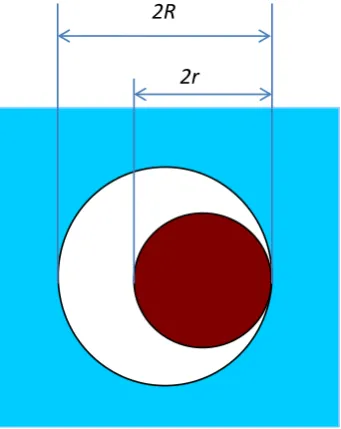
and refractive index n. The solute is represened by sphere of radius r which is determined according to the Dejardin et al. procedure [7]: dependence should be built of molar volume of the solute substance in liquid state on its fluidity at dif-ferent temperatures V0, the volume at the fluidity equal to zero, is connected

with r by equation

( )

1 3 0

pac

(3)

Here kpac is packing factor. It equals to 1.88 for molecules whose shape does

not sufficiently differ from spherical (Figure 1).

2.2. Interactions in the Solution and the Spectral Shift

There are two sorts of interactions in a dilute aqueous solution of nonpolar sub-stance: solute-solvent and solvent-solvent interactions. Only the first one affects directly the spectral shift whereas the second of them affects indirectly partici-pating in organization distribution solvent molecules around the solute. An electronic spectrum can be used for study the solution structure rather than vi-brational one because in contrast to vivi-brational spectrum it belongs to whole molecule rather than to some of its fragments. Let the simplest case of the solute will be considered, when the solute is nonpolar molecule, and let electronic ab-sorption of the solute is far from the solvent edge of the solvent abab-sorption and let solute electronic states are mutually independent. Then the shift of a purely electronic or electronic-vibrational (vibronic) band in the transfer of a molecule from the gas phase to the solution may be considered as sum of the different contributions:

disp elst chem

ν ν ν ν

∆ = ∆ + ∆ + ∆ (3)

Here ∆ν is the shift of the spectral band expressed in wave numbers, ∆νdisp

is contribution from dispersion interactions of the solute with solvent molecules,

elst

ν

∆ _{is that part of the shift which is determined by interaction with sources of}

constant electric fields (ions, dipoles,…) in the solvent, and ∆νchem is the term

[image:3.595.290.461.467.682.2]

which corresponds to those chemical interactions including hydrogen bonding that do not change individuality of the solute molecule.

Figure 1. Model, A solute (sphere of radius r)

in a spherical cavity of radius R created in the solvent.

(4)

Minimum of free energy of dispersion interaction take place when the solute touches the cavity border. The share of the shift stipulated by this type of inte-ractions is

(

,

) ( )

disp C R r f n

ν ϕ

∆ = − _{, (4)}

where C is a positive coefficient depending on properties of the transition in consideration,

_ϕ

( )

_{R r}_, ₌_R3 _r3

(

₂_{R r}₋

)

3

  is geometrical factor where R is

ra-dius of the cavity containing the solute molecule whose rara-dius is r,

( )

(

2 ₁

) (

2 ₂

)

f n = n − n + _,_n_{is refraction index}_[8]_.

It was shown in ref. [9] that there are neither electrical nor chemical interac-tions between the solute and the solvent in the aqueous solution of benzene. This fact will be used below at construction the simplest version of solubility model in which density fluctuations in the solute are taken into account.

This consideration is related to mutually independent electronic transitions. When electronic states are connected by a vibration, then the low which de-scribes the shift suffers changes [10][11]. So the shift of S1 − S0 benzene

transi-tion is approximately expressed as

( )10 1.910

1 10

C

ν ν

∆ = − ∆ _{, (5)}

where C1 is the positive coefficient, ∆ν10 is the shift in the absence of

electron-ic-vibrational coupling of the S1 electronic state with other ones, and index 1.910

is a correction for this coupling [12].

Solvents whose aromatic molecules contain oxygen make exciplexes with high-energy states of aromatic solutes [12]. This fact permits to solve reverse spectroscopy problem using only the most low-energy transitions at handling with such solvents.

2.3. Experimental Data

Experimental details including purification of substances, recording and mea-suring spectral shifts were done in refs. [9][10][11]. Data concerning solubili-ties are cited below.

3. Solubility

3.1. Microscopic Balance of Volumes

The average size of cavities in the solvent able to participate in the dissolution process can be found from balance of volumes at dissolution:

1vu av 1u bv E

V =V =V +V +V ₍₆₎

Here V1vu is average volume of that cavity in the solvent, (superscript v)

which contains one solute molecule (subscript 1u), Vav is the same volume in

the solvent obtained after removal a ofitsmolecules, V1u is average volume per

one solute molecule in the solute substance, Vbv is average volume of those

(5)

Solutions of benzene in different solvents can be considered as an instructive example. One obtains from Equation (5)

( )10 1/910

_{( ) ( )}

_,

disp kf n R r

ν

= −

ϕ

∆ ₍₇₎

where _k₌_{2824.9695422 cm}−1_and _r₌_{2.72 10 m}_× −10 _{. The results of}

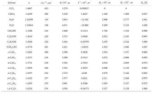
calcula-tion microscopic balance of volumes at benzene dissolucalcula-tion in different solvents are listed in Table 1.

It is readily seen from the Table that benzene forms simple intermixing only with carbon tetrachloride, Rbv=0, not with all other considered solvents where

0 bv

R > _{. The positive values of} R_bv witness that just cavities participate in dis-solution process, at least, in considered cases.

Next interesting consequence is seen from the Table. The excess volume plays negligible role In all considered cases. This fact supports conclusion made above that dissolution realizes through fluctuation cavities even in cases of infinite so-lubility, as for example in alkanes.

3.2. Minimal Radius of the Suitable Cavity

[image:5.595.51.544.424.726.2]

The minimal radius of the cavity yet participating in the process of benzene dissolu-tion can be evaluated from the funcdissolu-tion of cavity size distribudissolu-tion in the solvent [5]:

Table 1. Solvents, their refractive indices, n, shifts of benzene S1←S0 transition spectrum, ∆ν( )10 , average radii of cavities

containing a benzene molecule, R, excess volumes of mixing, _VE_{, averaged over different sources, and} bv

R is radius of average fluctuation cavity participating in dissolution and Rbv′ is the same without taking in consideration excess volume.

Solvent n _−∆_ν( )10_,cm−1 _R_×_{10 , m}10 _VE_×_{10 ,m}30 3 _{10 ,m}10

bv

R × ₁₀10

bv

R′× _{, m} R R_bv _bv′

CCl4 1.4607 433 3.279 0.030037 0 0

CHCl3 1.4459 386 3.329 1.4447 1.348 1.409 0.957

H2O 1.33299 145 3.815 −11.342 2.890 2.777 1.041

D2O 1.33844 128 4.011 −10.960 3.209 3.122 1.028

CH3OH 1.3288 210 3.408 0.1214 1.760 1.764 0.998

C2H5OH 1.3610 220 3.515 3.9448 2.032 2.105 0.965

C3H7OH 1.3850 234 3.563 −0.10793 2.235 2.216 1.009

(CH3)2SO 1.4770 381 3.431 −3.8325 1.932 1.846 1.047

c-C6H12 1.4262 368 3.306 4.5826 1.054 1.237 0.860

n-C5H12 1.3575 218 3.508 0.7415 2.072 2.086 0.993

n-C6H14 1.3751 238 3.502 2.7433 2.016 2.069 0.974

n-C7H16 1.3876 246 3.524 4.5033 2.048 2.130 0.962

n-C8H18 1.3975 254 3.535 4.649 2.078 2.160 0.962

n-C10H22 1.4102 257 3.577 3.6221 2.211 2.268 0.975

n-C14H30 1.4293 270 3.601 4.2366 2.263 2.327 0.972

(6)

( )

d d exp c

bv B

p= RR _−G R k T_₍₈₎

where c bv

G is average free energy of the fluctuation cavity surface which partic-ipate in dissolution (the same indexes are used in Equation (6)). It may be ex-pressed through microscopic surface tension [13][14]:

c

G =κγσ_{. (9)}

Here σ _{is the cavity surface area,} γ_{is the macroscopic surface tension, and}

κ is the coefficient correcting the macroscopic surface tension to the micro-scopic one. It is expressed as [13]:

(

1

)(

1

)

1 1

κ ≅ + σ σ κ − _{, (10)}

where σ1 is the area of the surface of the cavity created in the liquid as a result

of removal of one of its molecules, and

( )

1

(

)

1 1 k TB ln k T PVB s 1

κ γσ −

≅ _{. (11)}

Here Ps is pressure of saturated vapor and V1 is the volume per one

mole-cule in the liquid. For associated liquids

( )

1

(

)

1 1 k TB ln k T PVB ξ s 1

κ γσ −

≅ _{, (12)}

where ξ is average degree of association of vapor molecules [15]. Now Vbv can be expressed as

( )

3 2 2 d exp 4 d exp m m c B R _B bv m c B R

RR G R k T

k T

R R

RR G R k T

κγ

∞ ∞ −    = = + π −   

∫

(13)

Here Rm is the radius of that minimum cavity which is still good for

accep-tance the solute, γ =71.95 mN m _[16]_, κ ≈1 [15]. Hence

10 2.81 10 m m

R ₌ _× − _{. This value exceeds}_r₌_{2.72 10 m}_× −10 _[7]_{adopted here for}

benzene molecular radius only about 3%. This is too low difference for our crude model of solution. Therefore we may think that the minimal size of the cavity in water able to take the benzene molecule coincides with benzene molecule size. This conclusion is extended further to other big nonpolar solutes.

3.3. Approaches to Solubility

3.3.1. Fluctuation Approach

Let us consider low solubility of substance consisting of big nonpolar molecules, so low solubility that solute molecules do not touch each other. Let N is full amount of solvent molecules and n is amount of cavities able to accept a solute molecule. Then solubility is determined by

(

)

* _kT _ln _{n N} _ln_c

µ = − = − (14)

(7)

(

)

(

)

(

)

(

)

2

2 2

2

d exp 4

ln ln 4

d exp 4

e

B r

e e B

B r

RR R k T

n n r r k T

RR R k T

γ

γ γ

∞

− π

= = π −

− π

∫

. (15)

One obtains after substituting the right side of Equation (15) into Equation (14):

(

)

* * ₄ 2 2

e r re

µ′ =µ + πγ − ₍₁₆₎

Here prim numbers the approach to evaluation the solubility. The results ob-tained with this approach are given in the third column of Table 2. They are not very significantly deviated from empirical data. Note that this approach is not connected even with phase states of solution components.

3.3.2. Energetic Approach

Free energy of molecular transfer out of the fixed position in the substance which will be dissolved into the fixed position in vacuum and then into the fixed position in the solvent, _µ*_′′_{, is considered in the second approach called}

ener-getic one. In the idealized case when solute properties do not change at these transitions,

*

1ivu 1cvu 1iu 1cu

G G G G

µ ′′ = + − − ₍₁₇₎

Here G1ivu is free energy of interaction (superscript i) of one solute molecule

(subscript 1u) with the solvent (superscript v), G1cvu is free energy of creation

the cavity in the solvent (superscript c) where the solute molecule can be placed,

1iu

G is free energy of interaction between the solute and its environment in the solute substance, and G1cu is free energy of creation the cavity instead removed

[image:7.595.206.537.527.736.2]

solute molecule. The detailed Equation (17) looks as

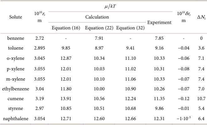
Table 2. Geometrical characteristics, quasi-chemical potentials of dissolution and

in-crease of aqueous molecules in the first hydrate cell of some substituted benzenes in water at 293 K.

Solute 10_m10r,

kT

µ

1010_δr, m ΔN1 Calculation

Experiment Equation (16) Equation (22) Equation (32)

benzene 2.72 - 7.91 - 7.85 - 0

toluene 2.895 9.85 8.97 9.41 9.16 −0.04 3.6 o-xylene 3.045 12.87 10.34 11.10 10.33 −0.06 7.1 p-xylene 3.055 12.01 10.03 11.02 10.31 −0.08 7.4 m-xylene 3.055 12.01 10.10 11.06 10.33 −0.07 7.4 ethylbenzene 3.04 11.80 10.00 10.90 10.26 −0.07 7.0 cumene 3.19 13.91 10.56 12.24 11.35 −0.12 10.7

(8)

DOI: 10.4236/ojpc.2019.94012 211 Open Journal of Physical Chemistry *

1 1

i i c i c i c

av av bv bv u u

G G G G G G G

µ ′′ = + ∆ + − − − − ₍₁₈₎

where i av

G is free energy of interaction between content of sphere which radius is R1vu before removal а solvent molecules out of it and the rest solvent, Gavc is

free energy of this cavity surface, terms with subscripts bv and1u describe simi-lar characteristics of original vacancies in the solvent and components of that free energy which must be spend for removal one molecule out of the substance to be dissolved, respectively, and _∆_Gi_{is a correction which must be}

intro-duced into the process description after replacement claster of a solvent mole-cules for one solute molecule. According to [13][14],

2

i c

G = − G ₍₁₉₎

and Equation (18) becomes simplified to

*

1

c c i c

av bv u

G G G G

µ′′ = − + + ∆ + ₍₂₀₎

When size of the cavity which contains the solute molecule is held rather by induced electrostatic forces than by collisions at thermal movement, then equili-brium takes place at

0

c c i

av bv

G G G

− + + ∆ = ₍₂₁₎

Then

* 1cu

G

µ′′ = ₍₂₂₎

In essence, _µ*_′′_{is pseudo chemical potential of transfere a molecule out of}

the condensed substance liable to dissolution into the solvent. It is described with the next equation:

* _kT _ln_C

µ′′ _{= −} _.₍₂₃₎

Thus it is the quasi chemical potential. The double prim numbers the ap-proach to evaluation _µ*_{. The data on calculated solubilities are given in the}

fourth column of Table 2. They also are close enough to empirical results. When the solute molecule is transferred out of a solid phase into the solvent then Equation (23) should be specified. Zhang and Gobas [17]supposed that a surface molecule of a solid substance dissolving in a liquid is bound with other ones in that manner as molecules of super cooled liquid. Then

(

)

*

1

ln s u f

kT RT p V G

µ

′′ = − ∆ (24)

Here ∆Gf is a change of free energy at conversation the solute substance into

the state of super cooled liquid which equals to

(

1

)

Tm d Tm d

f f m p p

T T

T

G H T T C T T C

T

∆ = ∆ − + ∆

_∫

−

_∫

∆ ₍₂₅₎

Here ∆Hf is enthalpy of solute substance fusion at melting point Tm and

p

C

(9)

square-law extrapolation specific heat of the liquid phase taking necessary values from ref. [18]: _{4.184 1.00286 10}

(

4 2 _2.2563 _{66.1362 J mol K}

)

p Т Т

C _× − ₋ ₊

∆ = ⋅ _.

3.3.3. United Approach

Corrections to solute size changes should be introduced in both two above de-scribed approaches. Correcting term δµ′_{to the quasi-chemical potential}_µ*_′

is caused by the molecular size decreasing because of pressing by reaction field forces [9]. It can be found from the next expression:

(

)

(

)

* *

2

* 2

* 2 2

4

4 2

e

e e

r r r

r r r r

µ

δµ

µ

δ

γ

µ

δ

γ

′= ′+ ′

 

′

= + π_ + − _

′

≅ + π + −

(26)

and

8 r r

δµ′ πγ δ . (27)

Such correction is the negative value because its sign coincides with the sign of

r

δ .

Correction to µ′′ in energetic approach looks as

* *

µ_{′′ =}µ′′₊δµ′′₍₂₈₎

where _{δµ ′′}* _{is correction which takes into account reversible positive work}

making by forces of hydrophobic (electric) repulsion which compress the solute molecule.

(

)

* 2 2

1

4 R R

δµ′′ ≈ πγ − ₍₂₉₎

Here R1 is radius of the cavity containing the solute in the case if it is not

subjected to deformation, and R is the same after deformation. R can be ex-pressed in quasi-spherical approximation as 3 3

(

)

3 1 3

1

R₌R r_{− + +}r δr 

  . We get

after expansion R in the Tailor series and taking into account that R≈3 2r _,

and neglecting the infinitesimal terms of decomposition, that

* ₈ _{r r}

δµ′′ ≈ − πγ δ ₍₃₀₎

One obtains comparing Equations. (27) and (30) that

* *

δµ′_{= −}δµ′′₍₃₁₎

It follows from Equation (31) that difference between values _µ*_′_and _µ*_′′_is

caused only by contraction of substituent size under reaction (reactive field) of the aqueous solvent on the solute. Hence

(

)

* * * ₂

µ

=

µ

′+

µ

′′ ₍₃₂₎

Only deformation of the solute is taken into consideration at calculating _µ*_.

The value of the solute size contraction is

(

16

)

r r

(10)

where _{∆ =}_{µ µ}*_′₋_µ*_′′_.

The values of _µ*_{with values of} _δ_r_{are given in the fifth column of}_{Table 2}_.

Firstly, it is readily seen from the Table that the predicted values of _µ*_are

closer to the measured ones then predicted by any of above approaches. So the main points of presented consideration look right. Secondly, the substance with rigid molecules, namely naphthalene, does not show any size contraction under aqueous solvent influence. Contractions show molecules containing alkyl subs-tituents. The more branched is a substituent, the more is contraction. This fact is evidently caused by facility of ordinary bond deformation.

3.3.4. Taking into Account Solvent Shell Strengthening

Interaction between water molecules in hydrate shell of benzene molecule is more strong then in pure water. Really, ions K+_{and Cl}-_{destroy water structure,}

i.e., weaken interaction between the molecule and other water molecules [19]. Nevertheless, addition salt KCl into aqueous solution of benzene does not de-stroys its hydrate cell, in contrast to addition such salts as RbCl and CsCl [9]

which are more actively then KCl [19].

One can evaluate contribution of this enhancement into the μ* value compar-ing calculated values with measured ones. The correspondcompar-ing correction equals to

*

1

0.214 0.055

kT N

µ

∆ = − ∆ + ₍₃₄₎

Here N1 is amount of water molecules in the first hydrate shell of benzene

and ∆N1 is the change of this amount after transition to another solute.

Ap-proximately

( )

1 3 2

( )

2 3

1 4 1u 2 1u

N = π_R V+ _ V _{, (35)}

where R≈1.5r . The correlation factor of dependence (34) equals to

0.943

ρ= _{, of root mean square deviation of coefficient at}∆N₁ σ =A 0.080

and of free term σ =В 0.028. One can readily see from Equation (34) that

inte-raction between water molecules in the first hydrate shell is enhanced owing to interaction with the solute and lowering the solvent free energy per one its mo-lecule in the solvent shell equals approximately 0.2kT. The low value of the free term in the right side of Equation (34) witness that adopted approximation is correct (see Table 3).

4. Conclusions

The above consideration clearly shows that fluctuations of density such as va-cancies (holes, cavities) in diverse solvents should be taken into account at eval-uations solubility of different solutes. This fact leads to paradoxy at the first glance conclusion that the excess volume plays a very modest role in microscop-ic balance of volumes at dissolution process, at least, in considered cases.

(11)

[image:11.595.56.543.100.279.2]

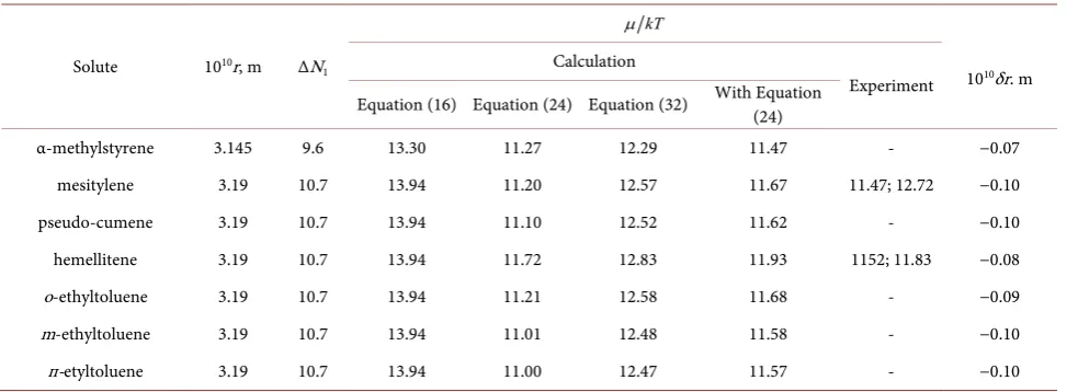
Table 3. Geometrical characteristics and quasi-chemical potentials of dissolution of some alkyl substituted benzenes in water at

293 K and solute contractions.

Solute 1010_{r, m} _ΔN 1

kT

µ

1010_{δr. m} Calculation

Experiment Equation (16) Equation (24) Equation (32) With Equation ₍₂₄₎

α-methylstyrene 3.145 9.6 13.30 11.27 12.29 11.47 - −0.07

mesitylene 3.19 10.7 13.94 11.20 12.57 11.67 11.47; 12.72 −0.10

pseudo-cumene 3.19 10.7 13.94 11.10 12.52 11.62 - −0.10

hemellitene 3.19 10.7 13.94 11.72 12.83 11.93 1152; 11.83 −0.08

о-ethyltoluene 3.19 10.7 13.94 11.21 12.58 11.68 - −0.09

m-ethyltoluene 3.19 10.7 13.94 11.01 12.48 11.58 - −0.10

п-etyltoluene 3.19 10.7 13.94 11.00 12.47 11.57 - −0.10

changes, and change of strength of hydrogen bonds in the solvent near the so-lutes look right. So, the main points of the above consideration are correct.

In essence, the called conclusions are obtained owing to taking into account, evidently or not evidently, effect of electric field described in ref. [9]. Hence such effect should be taken into consideration in advanced models of solubility, in-cluding computer simulation.

Conflicts of Interest

The author declares no conflicts of interest regarding the publication of this pa-per.

References

[1] Hildebrand, J.H. (1916) Solubility. Journal of the American Chemical Society, 38, 1452-1473.https://doi.org/10.1021/ja02265a002

[2] Hansen, C.M. (2000) Hansen Solubility Parameters. A User’s Handbook. CRC Press, Boca Raton, London, New York, Washington DC.

[3] Ben-Naim, A. (2006) Molecular Theory of Solutions. Oxford University Press, Oxford.

[4] Graziano, G.J. (1998) On the Size Dependence of Hydrophobic Hydration. Journal of the Chemical Society, Faraday Transactions, 94, 3345-3352.

https://doi.org/10.1039/a805733h

[5] Frenkel, Y.I. (1975) Kinetic Theory of Liquids. Nauka, Leningrad.

[6] Luck, W.A.P. (1981) Einfache Modelle für kalorische Eigenschaften der Flüssigkeiten.

Berichte der Bunsengesellschaft für physikalische Chemie, 83, 859.

[7] Dejardin, L.J., Marrony, R., Delseny, C., Brunet, S. and Berge, R. (1981) ne nouvelle définition des volumes libres dans les liquides non associés: Application à la déter-mination des diamètres moléculaires. Rheologica Acta, 20, 497-500.

https://doi.org/10.1007/BF01503272

[8] Ar’ev, I.A. (1987) Investigation the benzene hydration with spectral shift method.

(12)

DOI: 10.4236/ojpc.2019.94012 215 Open Journal of Physical Chemistry [9] Ar’ev, I.A. and Chernova, L.G. (2011) Interaction of Benzene with Water and

Aqueous Solutions of Alkali Metal Chlorides. Russian Journal of Physical Chemistry A, 85, 1592.https://doi.org/10.1134/S0036024411090032

[10] Ar’ev, I.A., Dyadyusha, G.G. and Makhlinets, N.V. (1983) Effect of Spin-Orbital In-teraction in Mono- and p-Dihalogenobezene Molecule on Their Electronic Spec-trum Shifts under Solvent Action. Optics and Spectroscopy, 55, 285.

[11] Ar’ev, I.A., Dyadyusha, G.G., Klimusheva, G.V. and Soroka, G.M. (1983) Effect of Spin-Orbital Interaction in Mono- and p-Dihalogenobenzenes in the S1 State under the Action of Environment. Optics and Spectroscopy, 55, 653.

[12] Ar’ev, I.A., Lebovka, N.I. and Solovieva, E.A. (2013) Effects of Partial Charge-Transfer Solute—Solvent Interactions in Absorption Spectra of Aromatic Hydrocarbons in Aqueous and Alcoholic Solutions. Molecular Physics, 111, 3077-3080.

https://doi.org/10.1080/00268976.2013.770175

[13] Sinanoglu, O. (1981) Microscopic Surface Tension down to Molecular Dimensions and Microthermodynamic Surface Areas of Molecules or Clusters. The Journal of Chemical Physics, 75, 463.https://doi.org/10.1063/1.441807

[14] Sinanoglu, O. (1981) What Size Cluster Is Like a Surface? Chemical Physics Letters, 81, 188-190.https://doi.org/10.1016/0009-2614(81)80233-3

[15] Ar’ev, I.A. (2014) Correcting the Microscopic Coefficient of Surface Tension of As-sociated Liquids. Russian Journal of Physical Chemistry A, 88, 173-174.

https://doi.org/10.1134/S003602441401004X

[16] Vargaftik, N.B., Volyak, L.D. and Volkov, B.N. (1975) Surface Tension of Water at Temperatures from 0 up to 370 Degrees of Celsium. In: Surface Phenomena in Liq-uids, Leningrad University, Leningrad, 180-192. (In Russian)

[17] Zhang, X. and Gobas, F.A.P.C. (1995) A Thermodynamic Analysis of the Relation-ships between Molecular Size, Hydrophobicity, Aqueous Solubility and Octa-nol=Water Partitioning of Organic Chemicals. Chemosphere, 31, 3501.

[18] Nikolskii, B.P. (1966) Handbook for Chemist. Vol. 1, 2, Khimia, Moscow, Lenin-grad. (In Russian)