The isolation of spatial patterning modes in a
mathematical model of juxtacrine cell signalling
O’Dea, R.D.∗ & King, J.R.
Centre for Mathematical Medicine and Biology, School of Mathematical Sciences,
University of Nottingham, University Park, Nottingham, NG7 2RD, UK
June 11, 2015
Abstract
Juxtacrine signalling mechanisms are known to be crucial in tissue and or-gan development, leading to spatial patterns in gene expression. We investi-gate the patterning behaviour of a discrete model of juxtacrine cell signalling due to Owen & Sherratt (Math. Biosci., 1998, 153(2):125–150) in which lig-and molecules, unoccupied receptors lig-and bound liglig-and-receptor complexes are modelled. Feedback between the ligand and receptor production and the level of bound receptors is incorporated. By isolating two parameters associated with the feedback strength and employing numerical simulation, linear stability and bifurcation analysis, the pattern-forming behaviour of the model is anal-ysed under regimes corresponding to lateral inhibition and induction. Linear analysis of this model fails to capture the patterning behaviour exhibited in numerical simulations. Via bifurcation analysis we show that, since the major-ity of periodic patterns fold subcritically from the homogeneous steady state, a wide variety of stable patterns exists at a given parameter set, providing an explanation for this failure. The dominant pattern is isolated via numerical simulation. Additionally, by sampling patterns of non-integer wavelength on a discrete mesh, we highlight a disparity between the continuous and discrete representations of signalling mechanisms: in the continuous case, patterns of arbitrary wavelength are possible, while sampling such patterns on a discrete mesh leads to longer wavelength harmonics being selected where the wavelength is rational; in the irrational case, the resulting aperiodic patterns exhibit ‘local periodicity’, being constructed from distorted stable shorter-wavelength pat-terns. This feature is consistent with experimentally observed patterns, which typically display approximate short-range periodicity with defects.
1
Introduction
Cell-to-cell communication plays a key role in the development of multicellular
or-ganisms (Hartenstein & Posakony, 1990; Keener & Sneyd, 1998; Mitsiadis et al.,
∗Corresponding author email: [email protected]; Current address: School of Science and
1999), leading to spatial patterns in gene expression that impact upon cell differ-entiation, the determination of cell fate and, ultimately, the development of tissues and organs. The activity of cell signalling molecules is typically divided into four distinct groups, termed autocrine, paracrine, endocrine and juxtacrine. The first three refer, respectively, to scenarios in which a cell produces a signalling molecule which is free to move within the tissue and acts (i) on the same cell, (ii) on a group of neighbouring cells (typically via diffusion) and (iii) on all cells within a tissue (as is the case with hormones). In contrast, juxtacrine signalling refers to the case where the signalling molecule is anchored in the cell membrane and acts only on neigh-bouring cells. The efficacy of such a mechanism is accordingly limited to closely packed structures such as epithelia.
Due to their importance in tissue development, cell signalling mechanisms have been the subject of a large number of theoretical studies. In this paper, we con-centrate on a discrete mathematical model for juxtacrine signalling; a review of
alternative cell signalling models is therefore omitted (see, e.g., Pribyl et al. (2003)
and Muratov & Shvartsman (2004) for discrete analyses of autocrine signalling). The study of Turing (1952), which showed that reaction and diffusion of chemi-cals can produce spatial patterning in chemical concentration that consequently de-termines cell fate, has inspired many authors to employ continuum reaction-diffusion models to study patterning in biological systems (though we note that Turing (1952) exploited both discrete and continuous formulations) – see, for instance, Wolpert
(1969), Painter et al. (1999) and Lander et al. (2002). Such models are posed in
terms of partial differential equations and as such analytic or asymptotic solutions may sometimes be obtained, as well as numerical-simulation approaches undertaken. However, the above continuum studies are inappropriate for small numbers of cells or for the study of fine-grained patterns in which variation takes place over few cell diameters. For these reasons discrete models are often used, taking the form of sys-tems of ordinary differential equations (ODEs) defined at discrete points in space, representing individual cells. The ease with which short range patterns and individ-ual cell behaviour or movement may be captured in such models has led them to be widely exploited to model many aspects of cell behaviour. The analysis of discrete models can rely heavily on numerical simulation, leading to an upper limit on the size of the problem that can be investigated; additionally, analytical results may be difficult or impossible to obtain from a discrete model considering realistic numbers of cells. Some authors have therefore attempted to derive continuum models based
upon an underlying discrete system. Examples include Turner et al. (2004), who
showed that, in the continuum limit, a Potts model of cell movement may be rep-resented by a diffusion equation, and O’Dea & King (2011a,b) in which multiscale continuum models capable of describing certain short-range patterns in square and hexagonal cells brought about by a simple juxtacrine signalling were formulated. We note that the techniques presented in these studies may be applied to the more complex model analysed herein; the calculation is summarised within the Appendix. A mathematical model for juxtacrine signalling was first considered by Collier
et al.(1996), concentrating on the activity of a transmembrane protein, Delta, and its receptor, Notch. Lateral inhibition, a negative feedback mechanism by which a cell adopting a particular fate inhibits neighbouring cells from doing likewise (Goriely
cell fate control mechanism (Mitsiadis et al., 1999), creating fine-grained patterns in developing tissue which determine subsequent cell development.
Plahte (2001) provided a comprehensive analysis of pattern formation in
contin-uous and discrete systems, with application to the model of Collieret al.(1996) and
concluded that linear analysis may not provide sufficient information to explain pat-terning behaviour. Plahte & Øyehaug (2007) suggests that in one spatial dimension, travelling waves invading an unstable homogeneous state may only generate period-two patterns, providing an explanation for the robustness of fine-grained patterning in this system.
Owen & Sherratt (1998) analysed a more complicated juxtacrine signalling model, considering the numbers of ligand and free and bound receptors. Lateral induc-tion (positive feedback between ligand-receptor binding and subsequent ligand pro-duction) was accommodated and the range over which juxtacrine signals may be transmitted was studied. Lateral induction is well-documented for a number of
ligand-receptor interactions, including, for instance, the binding of cAMP to
Dic-tyostelium cells (Owen & Sherratt (1998) and references therein). In a subsequent
paper, Owen et al.(1999) employed both a discrete (identical to that presented in
Owen & Sherratt (1998)) and a continuous formulation to investigate the propa-gation of signals in a juxtacrine signalling system, demonstrating that arbitrarily large signal half-lives are achievable and showing good agreement between the
dif-ferent modelling strategies. Wearing et al. (2000) analysed the model of Owen &
Sherratt (1998) further, performing an extended linear analysis to describe the pat-terning behaviour of the model and derived an approximation to the fastest-growing
patterning modes (i.e.those which one might expect to observe in nonlinear
simula-tions) for different regions of parameter space. However, the linear predictions failed to capture the qualitative behaviour of the nonlinear system. Motivated by this, Wearing & Sherratt (2001) performed a nonlinear analysis of a two-cell system, to-gether with bifurcation analysis to gain insights into the behaviour of larger systems, highlighting that linear analysis alone is unable to predict the model’s behaviour. Furthermore, this study concluded that the fine-grained patterns with approximate periodicity one sees in early development are due to the patterning dynamics rather than environmental inhomogeneity. Webb & Owen (2004) extended this signalling model, considering lateral induction and inhibition (up- and down-regulation of lig-and or receptor production in response to binding) in systems of varying geometry; specifically, one-dimensional strings and arrays of square or hexagonal cells were considered. Via linear analysis, the fastest growing modes were again calculated explicitly.
In this paper, we extend the work of Wearinget al.(2000) and Wearing &
numer-ical simulations run to steady state (from a variety of initial signalling profiles) in both the spatial and frequency domains, the dominant pattern for a given parame-ter choice is discerned. Finally, by sampling patparame-terns of non-integer wavelength on a discrete mesh, we show how the continuous and discrete representations of such signalling mechanisms may differ: in the continuous case, patterns of arbitrary wave-length may be generated which do not necessarily fit onto a discrete lattice, while in the discrete case such patterns result in longer wavelength harmonics being selected where the wavelength is rational; in the case of initial conditions of irrational pattern wavelength, the resulting pattern is found to be aperiodic.
The remainder of the paper is organised as follows. In§2.1, the model of Owen &
Sherratt (1998) is recapitulated; the linear stability properties presented in Wearing
et al. (2000) are summarised in §2.2. In §3 bifurcation diagrams and numerical simulations, together with spatial and spectral analyses, are presented to illustrate the emergence and dominance of different patterning modes in parameter space. In
§4, the evolution of patterns of non-integer wavelength is considered, showing how
the continuous and discrete representations of such systems may deviate. In §5, a
discussion of our results is given together with directions for future research.
2
A mathematical model of juxtacrine cell signalling
with feedback
2.1 Formulation
In Owen & Sherratt (1998), a model of juxtacrine cell signalling is presented. Such signalling is known to be of importance within closely packed cell populations, al-lowing membrane-bound signalling molecules to bind to receptors in adjacent cell membranes.
The mathematical model comprises ODEs which describe ligand-receptor
bind-ing on each cell and is expressed in terms of the numbers of ligand molecules aj(t),
unoccupied receptorsfj(t) and bound receptor-ligand complexesbj(t) on each cellj.
A generic model is employed to represent ligand binding in which it is assumed that a single ligand molecule binds reversibly to a receptor on the cell surface, giving rise to an occupied receptor which is subsequently internalised within the cell. In prac-tice new ligand and receptors are produced via recycling, release from intracellular
stores, and de novo production; however, in Owen & Sherratt (1998), the
simpli-fying assumption was made that the cell’s ligand and receptor production depends upon the level of occupied receptors in a prescribed way. By varying parameters associated with the feedback between ligand or receptor production and the level of bound receptors on a cell, up- or down-regulation of ligand and receptor production (known as lateral induction and inhibition) may be modelled.
The equations governing the evolution of ligand and free and bound receptors
on each cell j are, respectively (Owen & Sherratt, 1998):
˙
aj =−kaajhfji+kdhbji −daaj+Pa(bj), (1)
˙
fj =−kahajifj+kdbj−dffj+Pf(bj), (2)
˙
bj =kahajifj−(kd+ki)bj, (3)
rates of ligand binding and dissociation, ki the rate of ligand-receptor complex
in-ternalisation andda anddf are the rates of decay of ligand and free receptors. The
average over neighbouring cells is denoted h·iand defined by
hψji=
ψj−1+ 2ψj +ψj+1
4 , (4)
corresponding to an average over a two-dimensional array of square cells with
vari-ation in one dimension only. The functions Pa(bj),Pf(bj) represent the production
of ligand and free receptors and are specified as follows:
Pa(x) =
Cm 1 xm
C2m+xm, Pf(x) =C3+
Cn 4xn
C5n+xn, (5)
so that lateral inhibition or induction is captured by appropriate choice of the
pa-rametersC1−C5 and the exponentsm, n and was exploited in Wearing & Sherratt
(2001); e.g. C2m <0 leads to inhibition of ligand production in response to
ligand-receptor binding.
The data available on production rates of ligand and receptors are typically ex-tremely limited; however, the parameters in (5) may be specified to some extent, as follows (see Owen & Sherratt (1998)). Equilibrium levels of free and bound receptors are frequently known for specific biological systems; defining background receptor
expression r0 and spatially-homogeneous steady-states (f∗, b∗) specifies the
remain-ing steady-state, a∗, and three relations between the parameters in (5), leaving four
parameters unspecified C2, m and C5, n, which reflect the strength of feedback
in ligand and free receptor production, respectively. We choose C2 and C5 as free
parameters with which to investigate the model’s patterning behaviour in regimes corresponding to both lateral induction and inhibition, and fix the exponents to take
the valuesn=m= 3; similar behaviour may be obtained by varying the exponents
m and n. In vivo, ligand-receptor binding and the resulting ligand expression are dependent on the cell’s biochemical and biophysical environment; experimental ev-idence suggests that such environmental inhomogeneities are significant, providing motivation for the consideration the range of patterns produced by this model under variation of the feedback parameters.
2.2 Linear stability analysis
By expanding around the homogeneous steady states Owen & Sherratt (1998) and
Wearinget al.(2000) showed that the values ofP′
a(b∗),Pf′(b∗) (here denotedA, F,
respectively) dictate the behaviour of solutions; varying the parameters C2 and C5
allows us to proceed in A-F space to obtain different model behaviour. Curves
separating different patterning solutions were defined in the A-F plane as follows
(see Wearinget al. (2000) for details).
Linearising about the steady state via (aj, fj, bj) = (a∗, f∗, b∗) +δ(a1j, f1j, b1j)
and seeking solutions of the form a1j = aeσt+ikj (where a is constant, σ is the
temporal growth rate andk is the wavenumber), yields a cubic dispersion relation:
σ3+α1σ2+α2(K)σ+α3(K) = 0, (6)
wherein α1, α2 and α3 are functions (omitted; see equation (6), Wearing et al.
of the gradientsA, F and (except for α1) of the wavenumber k, via:
K(k) = cos(k) + 1
2 . (7)
Contours of neutral stability and of maximal instability in A-F space for each
wavenumber may easily be obtained from equation (6), indicating the regions of feedback parameter space in which the homogeneous state becomes linearly unstable to different pattern wavelengths. Maximal instability contours for a similar system are presented in Webb & Owen (2004) and an approximation to those corresponding
to equation (6) in Wearing et al. (2000).
The regions of parameter space in which linear analysis predicts spatial pattering are determined by analysis of the dispersion relation (6). This analysis was
previ-ously presented in Owen & Sherratt (1998) and Wearing et al. (2000) so we omit
the details. Referring to Figure 1, the results are summarised as follows:
1. Stability to homogeneous perturbations demands that the roots of (6) have
negative real part, requiring α1 > 0, α3(1) > 0 and α1α2(1)−α3(1) > 0.
These conditions define two straight lines in theA-F plane (denotedL1 and
L2, respectively) delimiting the stable region.
2. Instability to inhomogeneous perturbations requires at least one positive root
of (6), corresponding to α1α2(K) <0 or α3(K) <0. These conditions yield
a straight line L3 as well as a curve, C which bounds the region in which
complex roots are obtained. A further line L4 divides the stable region into
two parts. This line bounds the region in which the smallest root ofα3(K) is
zero.
3. The wavelength of the fastest growing modes in region II is bounded along
the line L4, above which K ∈
0,12
; i.e. the fastest growing wavelength is
λ∈[2,4). Wavelengths of two or three cells are therefore expected to dominate
the pattern form; no such restriction is found for values ofF lying below the
line L4.
Figure 1(a) shows a sketch of the A-F plane illustrating the regions defined
by the lines L1–L4 and the curve C. Figure 1(b) shows a numerically calculated
version of this stability diagram with neutral stability contours superimposed (cal-culated from equation (6)). Below each of these contours, the homogeneous steady state is linearly stable to periodic perturbations of that period; above, the linear analysis predicts patterns forming. Figure 1(c) shows contours of the fastest grow-ing patterngrow-ing modes. We remark that the neutral stability contours shown in Figure 1(c), which indicate that longer range patterns are expected to emerge as the rate of free receptor production increases, are also consistent with the linear analysis of
Wearing et al. (2000), in which it is predicted that patterns of period 2 or 3 will
dominate in region II. By considering an alternative form for the nearest neighbour interaction (4), Webb & Owen (2004) obtained qualitatively different behaviour to
that shown in Figure 1(c); however, by suitable re-definition ofK, we may reproduce
F
A L1
L2
L3 L4
C
I II
III
(a)
−0.02 −0.015 −0.01 −0.005 0 0.0050.010.015 0.020.025 0.044
0.046 0.048 0.05 0.052 0.054
F
A
(b)
−0.02 −0.01 0 0.01 0.02 0.044
0.046 0.048 0.05 0.052 0.054
F
A
(c)
Figure 1: (a) A sketch of theA-F plane denoting the regions of stable homogeneous
solutions (I), stable periodic patterns (II) and instability of the homogeneous steady
state to homogeneous perturbations (III). Adapted from Wearing et al. (2000); (b)
neutral stability contours in theA-F plane for patterns of increasing periodλ= 2–8
(solid lines: period increases clockwise) and (c) contours of fastest-growing
pattern-ing modesλ= 2–7 (solid lines: period increases clockwise) together with the curves
L1,L3,L4 andC delimiting the regions in parameter space in which patterns may
be formed (dashed lines). Parameter values taken from Owen & Sherratt (1998):
ka = 0.0003molecules−1min−1,kd= 0.12min−1,ki= 0.019min−1,da= 0.006min−1,
df = 0.03min−1, f∗ = b∗ = 3000, except r0 = 2850, m = n= 3. The dotted box
in (b) shows the region of parameter space investigated in more detail in §3; the
asterisk indicates the parameter value employed in the numerical simulations shown in Figure 2.
3
Numerical simulations and bifurcation analysis
3.1 Pattern emergence and stability
The linear analysis of Wearing et al. (2000) and Webb & Owen (2004) enables
partitioning of parameter space into regions in which stable patterns are generated from the homogeneous steady state, and enables determination of the fastest-growing modes. However, the applicability of such a linear analysis depends on whether the bifurcation at which the pattern under consideration is created is of supercritical type; in the case of subcritical patterning bifurcations, the linear approximation fails to reflect the patterning dynamics. Indeed, numerical simulation of the nonlinear system reveals that the linear predictions fail (unsurprisingly) to capture even the qualitative patterning behaviour of the system. In the following section, we present numerical simulations, together with bifurcation diagrams, for parameter values corresponding to both lateral inhibition and induction to demonstrate the emergence of different regular patterning modes; furthermore, since the analysis of the fastest growing mode has proved a poor predictor of which patterns will dominate, we calculate via numerical simulation the dominant patterns for each parameter set for a range of initial data.
The system (1)–(3) is solved using the initial value problem solver ode15s in
[image:7.612.96.442.39.159.2]in the simulations performed and observed in early tissue development (Wearing & Sherratt, 2001).
0 10 20 30 40 50 60 70 80
350 400 450 500
0 10 20 30 40 50 60 70 80
2000 3000 4000 5000 6000 7000
0 10 20 30 40 50 60 70 80
1000 2000 3000 4000 5000 6000
a
f
b
[image:8.612.129.405.80.293.2]Cell number
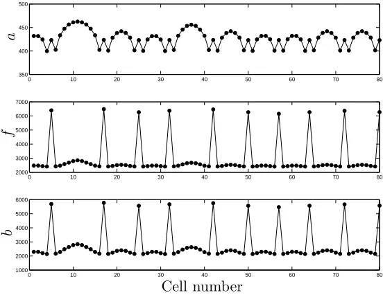
Figure 2: The steady-state pattern obtained from numerical simulation of the system
(1)–(3) att= 1000h in a line of 80 cells with periodic boundary condition indicating
that the patterns typically obtained from (1)–(3) display approximate periodicity
with defects. Parameter values are as in Figure 1 with C2 and C5 chosen such that
A,F lie in region II (as indicated by the asterisk in Figure 1(b)), in which stable
patterns are predicted by linear analysis. Initial conditions are random perturbations about the homogeneous steady states.
We now investigate the emergence of different regular pattering modes. The
system may, in principle, be driven towards a mode of arbitrary integer periodλby
choosing suitable periodic or near-periodic initial conditions and domain size, for an appropriate parameter choice at which such a mode is stable. We remark that tacit in the below is the assumption that only one such patterning mode exists (up to cyclic permutation); our numerical investigations suggest this to be the case. Figure 3 depicts sample bifurcation diagrams (together with sample simulation results)
for the system (1)–(3). Figures 3(a) and (c) illustrate the stability of the λ = 3
and λ = 4 patterns as the free receptor production parameter C5 is varied in the
diagrams on 8 cells are shown).
Figures 3(a) and (c) give an insight into why the linear analysis fails to give a complete description of the patterning behaviour of the system (1)–(3). Patterns may be formed in regions of parameter space below the relevant neutral stability curve predicted by the linear analysis (shown in Figure 1(b)) since the solution branches can fold subcritically from the homogeneous steady-state to form stable patterning regimes in regions of parameter space where the homogeneous state is linearly stable to periodic perturbations. An alternative mechanism for this phenom-ena is that the non-fastest-growing patterning mode is stable as a nonlinear pattern. We emphasise that since the uniform state is linearly stable to non-uniform pertur-bations, the competition between states that we are describing should be viewed in terms of bistability, rather than of a Turing pattern, for example, arising through propagation over an unstable state.
We pause here to note that, not only do the linear instability curves shown in Figure 1(b) fail to represent the emergence of patterns in the nonlinear system, but the fastest-growing modes shown in Figure 1(c) (often good predictors of observed patterning behaviour) are similarly inaccurate.
The supercritical pitchfork bifurcation which branches from the homogeneous
steady-state in Figure 3(c) represents the λ = 2 bifurcation which occurs as the
receptor production is increased across the line L4; see Figure 1(b) (separate plot
omitted for concision). This supercritical bifurcation, which exists for a wide range of parameter values corresponding to lateral inhibition, is exploited in the Appendix, in which a multiscale analysis is employed to demonstrate that complex discrete pattern-forming models of this type may be accommodated within tissue-scale rep-resentations; subcritical bifurcations typically preclude useful application of such an analysis since the unstable solutions reflected in the multiscale asymptotic equations
will not be observed in nonlinear simulations. For values ofC5/b∗ corresponding to
F lying above the lineL4 in theA −F plane, theλ= 4 pattern branches
subcrit-ically from the λ= 2 solution. Figure 4 shows how the λ= 4 pattern is generated
from the λ = 2 solution under variation of the ligand production parameter C2 in
the lateral inhibition regime: again, the λ= 4 solution branches subcritically from
the shorter period pattern.
3.2 Dominant patterning modes
As remarked above, linear analysis of the fastest growing modes proves a poor in-dicator of the pattern wavelengths generated by the full nonlinear system. We wish to determine the dominant pattern period for a given parameter choice; these were determined via numerical simulation as follows. Solutions to (1)–(3) were obtained,
from a series of initial states consisting of a patch of stable pattern of period λ
(of width 10λ cells) surrounded by the homogeneous state (so that a wide array
of pattern wavelengths are admitted, 120 additional cells are used). The resulting steady-state solutions were analysed in both the frequency and the spatial domains. Spectral analysis (or frequency domain analysis) provides a simple and power-ful way to identify the (spatial) frequency components in patterned solutions and is widely used in signal processing applications (though in these applications, the data usually take the form of a time-series, rather than a spatial distribution; see,
1.55 1.6 1.65 1.7 1.75 448
450 452 454 456 458 460 462 464 466
a
C5/b∗
(a)
0 2 4 6 8 10 12 443
444 445 446 447 448 449
a
Cell number
(b)
1.52 1.54 1.56 1.58 1.6 1.62 1.64 1.66 1.68
454 456 458 460 462 464 466
a
C5/b∗
(c)
0 2 4 6 8 10 12 14 16 435
440 445 450 455 460 465
a
Cell number
(d)
Figure 3: (a) and (c): Bifurcation diagrams illustrating the subcritical
bifurca-tion of the λ = 3, λ = 4 patterns for the number of ligand molecules a from the
homogeneous state for system (1)–(3) (solutions for bound and free receptors are omitted for brevity); (b) and (d) show sample numerical simulation illustrating the corresponding patterns generated in a line of 120 cells with periodic boundary
con-ditions and t = 1000h. Parameters as in Figure 1 except C2 = 1000 and in, (b),
(d), C5 = 1.59b∗. The supercritical pitchfork bifurcation which branches from the
[image:10.612.127.412.152.441.2]−2000 −1900 −1800 −1700 −1600 −1500 454
456 458 460 462 464 466 468 470 472
Period−2 (stable) Period−2 (unstable) Period−4 (stable) Period−4 (unstable)
a
(o
d
d
ce
ll
s)
C2
(a)
−2000 −1900 −1800 −1700 −1600 −1500
410 420 430 440 450 460 470
Period 2 (stable) Period 2 (unstable) Period 4 (stable) Period 4 (unstable)
a
(e
v
en
ce
ll
s)
C2
[image:11.612.125.411.42.175.2](b)
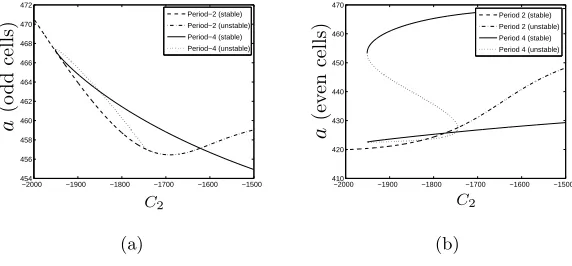
Figure 4: Bifurcation diagrams indicating how the period-4 pattern for ligand
con-centration branches from the period-two solution under variation of C2 on (a) odd
cells and (b) even cells. Stable and unstable period-two and four solutions are
indi-cated by the different line styles. Parameters as in Figure 3 except C5 = 1.6b∗ and
C2 as indicated.
is measured by the power spectral density, calculated as the scaled absolute value of the square of the discrete Fourier transform of the steady-state solution. The power spectral density is scaled so that its mean and variance are equal; the discrete Fourier
transform is obtained via the fft function in MATLAB. Energy peaks at distinct
frequencies indicate the presence (and prevalence) of different patterning modes. In the spatial domain, we calculate separately the stable periodic patterns that exist at each parameter choice and compare numerically these against the steady-state solutions obtained from time-dependent simulations, thereby providing an explicit measure of the appearance of different periodic cycles in the domain. By these two approaches we may isolate the different patterns that exist in the domain and cal-culate the dominant patterning mode for each parameter set: we characterise the dominance by the percentage of the domain occupied by that pattern.
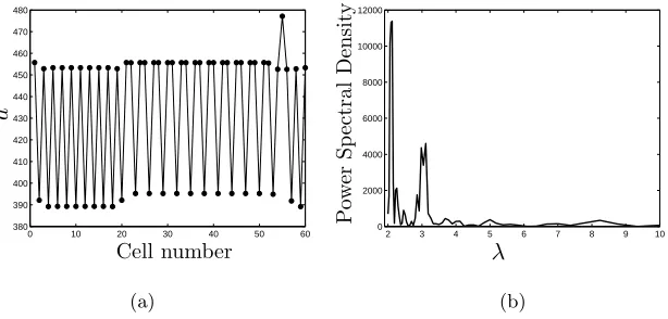
Figure 5(a) shows an illustrative steady state pattern in which both λ= 2 and
λ= 3 patterning modes coexist in the domain; Figure 5(b) indicates the power
spec-trum associated with this pattern, indicating how such an analysis clearly highlights
the patterning modes present via distinct peaks of power spectral density at λ= 2
and λ= 3. We remark further that it is relatively easy to construct patterned
solu-tions whose spatial distribution appears similar but whose spectrum shows distinct differences. This exemplifies the value of the spectral analysis method and further motivates the complementary use of both spatial and frequency domain analysis.
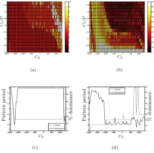
Figure 6 shows a plot of the dominant patterns in a region of A-F space
(cor-responding to the region of Figure 1(b) marked with a dotted box), together with its percentage dominance. For clarity, the axes are labelled with the values of the
feedback parameters C2 and C5 since the corresponding non-uniform A-F mesh
obscures detail near A = 0. Figures 6(c) and (d) show the dominant patterns for
two representative values of free receptor upregulation (C5 = 1.6b∗, 1.95b∗) together
0 10 20 30 40 50 60 380
390 400 410 420 430 440 450 460 470 480
Cell number
a
(a)
2 3 4 5 6 7 8 9 10
0 2000 4000 6000 8000 10000 12000
λ
P
ow
er
S
p
ec
tr
a
l
D
en
si
ty
(b)
Figure 5: (a) A section of a numerical simulation run to steady state in a periodic
line of 120 cells, in which λ = 2 and λ = 3 patterning modes are present. The
parameter values are as in Figure 3 exceptC5 = 1.85b∗,C2 =−1850. (b) The power
spectral density estimate corresponding to the simulation shown in (a).
Comparison of Figures 1(b,c) and 6(a) shows clearly that, due to the subcritical nature of the patterning bifurcations, patterns form in some regions of parameter space in which the homogeneous steady state is linearly stable to periodic pertur-bations. Furthermore, the fastest growing modes predicted by the linear analysis provide a poor description of the nonlinear behaviour, except for very strong ligand
inhibition at which λ= 2 patterns are predicted and observed. As the inhibition is
reducedλ= 3 and λ= 4 solutions achieve dominance. A region ofλ= 4 dominance
is observed between the λ= 2 and λ= 3 regions. Under induction, λ= 4 regains
dominance together with other, longer-wavelength patterns (λ = 5,6,9). Figures
6(b–d) indicate that the dominance of the patterns is greatly reduced for lateral
induction (A >0), the resulting patterns containing many defects. Comparison of
Figures 7 and 6(c,d) indicates that the same patterning trends are observed in the case for which the initial state comprises random perturbations to the homogeneous steady state: at strong inhibition, short range patterns dominate; longer-range pat-terns dominate under induction. We note that, apart from the case of very strong inhibition (in which the alternating pattern is robustly generated), the dominance of these patterning modes is very greatly reduced, and the resulting steady state pat-terns display mixtures of stable patterning modes with many defects (figure omitted). Combined, these results further exemplify that, with the emergence of more stable patterning modes (as inhibition is decreased), the predictions of the linear analysis shown in Figure 1 comprehensively fail to capture the nonlinear behaviour.
[image:12.612.122.429.41.188.2]values forms ongoing work, adding to existing investigations by, e.g.Owen (2002) .
−2000 −1500 −1000 −500 0 500 1000
1.6 1.65 1.7 1.75 1.8 1.85 1.9 1.95 0 1 2 3 4 5 6 7 8 9 10 C5 / b ∗ C2 (a)
−20001.6 −1500 −1000 −500 0 500 1000
1.65 1.7 1.75 1.8 1.85 1.9 1.95 0 10 20 30 40 50 60 70 80 90 100 C5 / b ∗ C2 (b)
−2000 −1500 −1000 −500 0 500 1000
2 2.5 3 3.5 4 4.5 5 5.5 6
−2000 −1500 −1000 −500 0 500 1000 40
50 60 70 80 90 100 Period Dominance C2 P a tt er n p er io d % d o m in a n ce (c)
−2000 −1500 −1000 −500 0 500 1000
2 3 4 5 6 7 8 9 10
−2000 −1500 −1000 −500 0 500 1000 0
10 20 30 40 50 60 70 80 Period Dominance C2 P a tt er n p er io d % d o m in a n ce (d)
Figure 6: (a) The dominant pattern period in a region ofA-F space, (b) the
per-centage of the domain occupied by that pattern as a measure of its dominance, and the dominant patterns for two representative values of free receptor upregulation
together with their percentage dominance: (c) C5 = 1.6b∗, (d) C5 = 1.95b∗.
Sim-ulations undertaken in a line of 10λ+ 120 cells with periodic boundary conditions.
Parameters as in Figure 3 exceptC2,C5 as indicated.
4
Non-integer patterns
The simulations presented in §3 demonstrate that many different stable patterns
exist at each parameter value; furthermore, the patterns generated from the
non-linear model do not adhere to the non-linear predictions presented in §2.2. In addition,
the resulting patterns generally contain defects. The linear analysis applies for both
continuous and discrete systems; as such, the wavenumber, k, is arbitrary and may
correspond to non-integer pattern wavelength. In the discrete case, this leads to patterns which do not fit onto the lattice. Below, we investigate the behaviour of such patterns, highlighting a point at which the equivalent discrete and continuum representations of signalling phenomena diverge.
[image:13.612.122.426.68.370.2]−2000 −1500 −1000 −500 0 500 1000 2 2.5 3 3.5 4 4.5 5 5.5 6
−2000 −1500 −1000 −500 0 500 1000 0
10 20 30 40 50 60 70 80 Period Dominance C2 P a tt er n p er io d % d o m in a n ce (a)
−2000 −1500 −1000 −500 0 500 1000
2 3 4 5 6 7 8 9
−2000 −1500 −1000 −500 0 500 1000 0
[image:14.612.125.424.42.173.2]10 20 30 40 50 60 70 Period Dominance C2 P a tt er n p er io d % d o m in a n ce (b)
Figure 7: Diagrams showing the dominant pattern, together with its percentage dominance resulting from an initial state comprising a region of random data sur-rounded by the unstable homogeneous steady state for for two representative values
of free receptor upregulation: (a)C5= 1.6b∗, (b)C5 = 1.95b∗. Other parameters as
in Figure 3 except C2 as indicated.
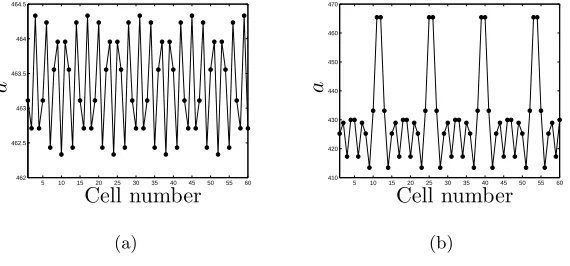
pattern of non-integer period sampled on the discrete mesh. Figure 8 shows initial
conditions of periodλ= 2.8 together with the resulting steady-state pattern.
Figure 8(a) illustrates how sampling patterns of rational non-integer wavelength
λ(with wavenumberk) on a discrete mesh leads to patterns of longer wavelength λ
(with wavenumber k) given by:
λ= 2
k; k= min{nk(mod2), 2−nk(mod2)}; λ, n∈Z. (8)
Equivalently, λ may be interpreted as the shortest integer multiple of the original
pattern that fits onto a discrete mesh;i.e.
λ=min{mλ}; wherem∈Zsatisfies mλ(mod2) = 0. (9)
Returning to the case for whichλ= 2.8, we findλ= 14 (n= 50,m= 6); inspection
of Figure 8 readily confirms this. Such wavelength selection ‘errors’ relate to aliasing effects observed in signal processing applications, in which the sampling frequency can cause signals of disparate wavelength to become indistinguishable.
We remark that Figure 8(b) indicates that the steady-state pattern of period
λ= 14 can, roughly speaking, be thought of as being constructed from (distorted)
patterns of shorter wavelength (here, patterns of period λ = 5 and λ = 3). We
note further that a straightforward linear analysis reveals that the homogeneous steady-state is stable to period-14 perturbations in the chosen parameter regime.
We therefore conclude that the λ = 14 pattern bifurcates subcritically from the
homogeneous steady-state in a similar manner to that shown in Figures 3(c) and 4 (we do not present a corresponding bifurcation diagram since the behaviour is exceedingly complex, with many solution branches).
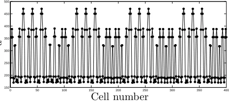
number of grid points used), numerical simulation suggests that the period of the resulting pattern becomes very large. For example, Equations (8), (9) predict
pat-terns of wavelength λ= 42426 from initial data of period λ= 2√2, truncated to 4
decimal places. However, we remark that the resulting pattern is ‘locally periodic’, consisting of smaller stable patterns that are stable at that choice of parameter value,
as was demonstrated for theλ= 14 pattern and shown in 8(b). Figure 9 shows the
pattern resulting from initial conditions ofλ= 2√2 (truncated to 4 decimal places).
The simulation was undertaken on an array of 3λ cells. The resulting distribution
of free ligand appears to display short-range periodicity; however, small defects in
the pattern mean that the true period, λ, is very much larger. This highlights a
disparity which can arise between the discrete and continuum representations of the same patterning system: in the continuum case, period-selection issues do not arise
and the wavenumber k is arbitrary; however, in the discrete model, initial data of
fractional (or irrational) period can result in the system evolving to surprisingly long-wavelength patterns. These patterns comprise smaller patterns that are stable at that choice of parameter value, with defects. These ‘locally periodic’ patterns are consistent with the patterns one observes experimentally; Wearing & Sherratt (2001) also observed such approximately periodic patterns, concluding that these are due to the patterning dynamics rather than environmental heterogeneity. The results presented in this section suggest that being driven towards a non-integer pat-terning state (via initial conditions and feedback characteristics) provides a simple explanation for the emergence of such patterns.
5 10 15 20 25 30 35 40 45 50 55 60 462
462.5 463 463.5 464 464.5
a
Cell number
(a)
5 10 15 20 25 30 35 40 45 50 55 60 410
420 430 440 450 460 470
a
Cell number
(b)
Figure 8: (a) Initial conditions corresponding to periodλ= 2.8 demonstrating the
λ = 14 periodicity on the discrete lattice, and (b) the eventual λ = 14 pattern
comprising distorted λ = 5 and λ = 3 patterns. C2 = 0, C5/b∗ = 2.8; other
parameters as in Figure 2.
5
Discussion
[image:15.612.128.413.352.485.2]0 50 100 150 200 250 300 350 400 150
200 250 300 350 400 450 500
a
[image:16.612.155.388.33.138.2]Cell number
Figure 9: The steady-state ligand pattern resulting from an initial state with period
λ= 2√2 (truncated to 4 decimal places). C2 = 0,C5= 2.8/b∗; other parameters as
in Figure 2.
on a cell and its production of new receptors and ligand was incorporated and, by varying two free parameters controlling the strength of this feedback, up- and down-regulation of receptor production (known as lateral inhibition or induction) were modelled.
Via a linear analysis, bifurcation analysis and numerical simulation, the variety of stable patterns which exist, for different feedback parameters was characterised. We demonstrated that the majority of bifurcations which generate different pattern-ing modes are subcritical (a supercritical pitchfork may be obtained in the period two case for certain parameter choices) and stable patterns may therefore be formed in regions of parameter space where the homogeneous state is stable to such periodic perturbations. This sheds light on the inability of the linear analysis to reflect the
observed behaviour of the nonlinear system, as reported in Wearing et al. (2000),
Wearing & Sherratt (2001) and Webb & Owen (2004) (and remarked in Plahte (2001) with regards to a simpler signalling model): at a given point in parameter space, a wide variety of stable patterns of disparate wavelengths exist overriding the wavelengths predicted by the linear analysis; indeed, we demonstrate that the fastest-growing linearly unstable modes (often good predictors of nonlinear pattern-ing behaviour) are inaccurate. By analyspattern-ing the results of numerical simulations in the spatial and frequency domains, the dominant pattern in a representative region of parameter space was determined, showing that shorter wavelengths dominate in the regime of lateral inhibition (and that the linear analysis is more successful at predicting the patterning behaviour in this regime), giving way to longer wavelength patterns with substantial defects under lateral induction.
however, they display ‘local periodicity’, being constructed from stable, shorter-wavelength patterns with defects. This highlights a disparity between the discrete and continuum representations of cell signalling systems. In the continuum case, such period-selection behaviour is not observed and patterns of arbitrary wavelength may be obtained, and, in general, nonlinearities will generate higher harmonics. Fur-thermore, other studies of this system (Wearing & Sherratt, 2001) have noted that the patterns created display, in general, short-range periodicity with many defects and that such patterns are consistent with those observed experimentally. Our anal-ysis of non-integer patterns indicates that such patterns emerge naturally when the system is driven towards a non-integer patterning mode via initial conditions and feedback characteristics.
Our results illustrate the following more general issues in analysing discrete pat-terning systems. We followed the usual procedure of performing a linear analysis in order to partition parameter space into regions in which different patterning modes might be expected to exist. However, given that many of the bifurcations in ques-tion are (as we have highlighted) subcritical, such a linear analysis does not provide an accurate description of the nonlinear behaviour; a thorough bifurcation analysis is thus required to indicate patterning behaviour. It is worth noting that the lin-ear analysis will be similarly ineffective if many (possibly generated at supercritical bifurcations) stable patterns exist for a given parameter set. For systems of this
type, thea priori linear analysis is insufficient and a numerical analysis of the type
employed herein is required. Numerical simulation of the model equations from a range of initial states together with a spatial- and/or frequency-domain analysis of the resulting steady-state patterns seem to represent the most effective ways to characterise the patterning behaviour.
The linear analysis summarised in this paper employs standard techniques. Wear-ing et al.(2000) noted that it is the specific form of the juxtacrine averaging term employed in this model (which corresponds to striped patterns in a square array) which distinguishes this patterning mechanism from Turing models, and that a term corresponding to discretised diffusion does not make sense biologically. However, it is markworthy that O’Dea & King (2011a,b) employed a homogenisation technique
to a simpler model of Delta-Notch signalling (Collier et al. (1996)) to show that,
on the tissue scale, the juxtacrine interaction does indeed manifest itself as linear diffusion, at least in the short-range patterning regime. In the Appendix, we show that the technique is applicable to more complex signalling models, paving the way for their incorporation into tissue-scale studies, by applying it to Equations (1)–(3). We further remark that this technique may only be usefully applied to patterns formed at supercritical bifurcations; the predominance of subcritical bifurcations in Equations (1)–(3) has, therefore, implications for the application of such methods to cell signalling models.
Acknowledgements
The authors gratefully acknowledge funding from BBSRC and EPSRC (BB/D008522/1). JRK also acknowledges the support of the Royal Society and Wolfson Foundation. All bifurcation diagrams were generated in XPPAUT v5.91.
A
A multiscale analysis of period-two patterns
In this appendix, we demonstrate that, in the period-two patterning regime, the discrete juxtacrine signalling mechanism manifests itself as linear diffusion on the macroscale. The method employed is that presented by O’Dea & King (2011a,b); the details are therefore omitted for brevity.
The results presented in this paper suggest that introducing appropriate spatial variation in the feedback parameters results in different patterning behaviour in cer-tain regions of the domain. In a specific biological context, such parameter variation would correspond to differences in the sensitivity of the cells to Delta-Notch binding, leading to the adoption of a particular programme of gene activation by a subset of the cell population according to spatial position.
To construct such a continuum model, a homogenisation process is required. We assume that the spatial variation of the chosen parameter is slow compared to the variation of ligand and free and bound receptor numbers, thereby preserving the local periodicity in the patterning regime; that is, we construct a two-scale model. Biologically, this corresponds to analysis of microscale pattern formation in response
to macroscale variation in cell-signalling activity (e.g. that induced by tissue-level
chemical or physical stimulation). Considering a line of cells, we denote the
dis-tance between cells byδ≪1 (see Figure 10), introduce a slowly-varying continuum
variable X = δj and slow timescale T = δct (where c > 0 is as yet unspecified)
and represent the numbers of ligand, free and bound receptors in the multiple-scales form aj = a(j, X, T), fj = f(j, X, T) and bj = b(j, X, T), in which j and X
rep-resent the rapidly-varying and the slow spatial scales, respectively. Additionally, since in the period-two patterning regime, neighbouring cells are expected to differ significantly in the numbers of ligand and free/bound receptors, we introduce the following notation to differentiate between “odd” and “even” cells:
ψ(j;X, T) =ψ+(X, T) j = 2i+ 1, (10)
ψ(j;X, T) =ψ−(X, T) j = 2i, (11)
where ψrepresents the numbers of ligand, bound and free receptors (a, f, b) and i
is an integer. Exploiting this notation and on expanding in Taylor series, the spatial
coupling term hψji defined by equation (4) may be written:
hψ±i= 1 2
ψ±(X, T) +ψ∓(X, T) +δ
2
2
∂2 ∂x2ψ
∓(X, T) +
O(δ4)
. (12)
In the following we derive coupled equations governing receptor and ligand activity in odd and even cells separately, facilitating the inclusion of fine-grained patterning phenomena within our continuum model.
j j+ 1
j−1 · · ·
· · ·
δ
X =δj
Figure 10: Definition sketch: a line of cells and the spatial coordinates employed in the multiscale analysis.
C2andC5, leading to variations in the gradient of the ligand and receptor production
functions, which control the patterning behaviour. Figure 3 shows that (for suitable
values ofC2) period-two solutions are created at a supercritical pitchfork bifurcation
on the line L4 (see Figure 1(a)); correspondingly, we expand aboutL4 such that:
Pf(k)(b∗, X;δ) =Pf(k)∗+δ2Fk(b∗, X) +· · · , (13)
ψ±(X, T;δ) =ψ∗+δψ1±(X, T) +δ2ψ2±(X, T) +· · · , (14)
wherein the superscript (k) denotes the kth derivative of Pf with respect to b (a
corresponding expansion is used for the ligand production rate Pa), and asterisks
denote the values of the feedback functions (and their derivatives) at the bifurcation
point on L4 at which ψ achieves its homogeneous steady-state ψ∗. Exploiting the
notation introduced in §2.2, we have A = Pa(1)∗ +δ2A1(b∗, X) and F = P(1)∗
f +
δ2F1(b∗, X); the points P(1)
∗
a , Pf(1)∗ lie on the line L4. For parameter choices
such that F1(b∗, X) 6 0, we therefore expect, as t → ∞, spatially-homogeneous
solutions to be approached; for F1(b∗, X) > 0, period-two solutions (generated at
the supercritical pitchfork) exist.
For clarity, we note further that the supercritical bifurcation under consideration exists for a range of parameter values corresponding to lateral inhibition; the analysis below may only be usefully applied in this case.
Combining the above expansions and choosingc= 2 (in order that both temporal
and spatial coupling appears in the O(δ) perturbation), and after some lengthy
algebra, we obtain the following partial differential equation for the number of bound receptors on odd cells:
∂b+1 ∂T = Λ
∂2b+1 ∂X2 +µb
+3
1 +νb+1. (15)
The remaining variables are calculated viaf1+=φb+1 anda+1 =χb+1 andψ1+=−ψ−1.
The parameters Λ,µ,ν,φ,ψandχare cumbersome functions of the model
parame-ters (ka, kd, da, df, ki), the steady-states (a∗, f∗, b∗) and associated branch point
feedback values and the perturbations to the feedback strength and are therefore
omitted for brevity. We remark, however, that the signs ofµand ν dictate the
pat-terning behaviour of the model. In particular, for constant µ,ν, the steady states
of (15) are b+1 = (0,±p
−ν/µ); for model parameter choices corresponding to F
below L4, only the trivial state exists (corresponding to the maintenance of the
homogeneous steady state); the change in sign ofµ,νfor parameter values at which
References
B. Appel, L.A. Givan and J.S. Eisen. 2001. Delta-Notch signaling and lateral
inhi-bition in zebrafish spinal cord development. BMC Dev. Biol, 1:1–13.
S.A. Broughton and K. Bryan. 2009. Discrete Fourier analysis and wavelets:
appli-cations to signal and image processing. Wiley-Interscience. ISBN 0470294663.
J.R. Collier, N.A.M. Monk, P.K. Maini and J.H. Lewis. 1996. Pattern formation by lateral inhibition with feedback: a mathematical model of Delta-Notch
intercellu-lar signalling. J. Theor. Biol., 183:429–446.
A. Goriely, N. Dumont, C. Dambly-Chaudiere and A. Ghysen. 1991. The determi-nation of sense organs in Drosophila: effect of the neurogenic mutations in the
embryo. Dev., 113:1395.
V. Hartenstein and J.W. Posakony. 1990. A dual function of the notch gene in
drosophila sensillum development. Dev. Biol., 142:13–30.
P. Heitzler and P. Simpson. 1991. The choice of cell fate in the epidermis of
Drosophila. Cell, 64:1083–1092.
J.P. Keener and J. Sneyd. 1998. Mathematical physiology. Springer New York.
A.D. Lander, Q. Nie and F.Y.M. Wan. 2002. Do morphogen gradients arise by
diffusion? Dev. Cell, 2:785–796.
T.A. Mitsiadis, K. Fried and C. Goridis. 1999. Reactivation of Delta–Notch signaling after injury: complementary expression patterns of ligand and receptor in dental
pulp. Experimental Cell Res., 246:312–318.
C.B. Muratov and S.Y. Shvartsman. 2004. Signal propagation and failure in discrete
autocrine relays. Phys. Rev. Lett., 93:118101(1–4).
R.D. O’Dea and J.R. King. 2011a. Continuum limits of pattern formation in
hexagonal-cell monolayers. J. Math. Biol. DOI: 10.1007/s00285-011-0427-3.
R.D. O’Dea and J.R. King. 2011b. Multiscale analysis of pattern formation via
intercellular signalling. Math. Biosci., 231:172–185.
M.R. Owen. 2002. Waves and propagation failure in discrete space models with
nonlinear coupling and feedback. Phys. D: Nonlin. Phenomena, 173:59–76.
M.R. Owen and J.A. Sherratt. 1998. Mathematical modelling of juxtacrine cell
signalling. Math. Biosci., 153:125–150.
M.R. Owen, J.A. Sherratt and S.R. Myers. 1999. How far can a juxtacrine signal
travel? Proc. Royal Soc. B: Biol. Sci., 266:579–585.
K.J. Painter, P.K. Maini and H.G. Othmer. 1999. Stripe formation in juvenile
Po-macanthus explained by a generalized Turing mechanism with chemotaxis. Proc.
E. Plahte. 2001. Pattern formation in discrete cell lattices. J. Math. Biol., 43(5): 411–445.
E. Plahte and L. Øyehaug. 2007. Pattern-generating travelling waves in a discrete
multicellular system with lateral inhibition. Phys. D: Nonlin. Phenomena, 226
(2):117–128.
M. Pribyl, C.B. Muratov and S.Y. Shvartsman. 2003. Discrete models of autocrine
cell communication in epithelial layers. Biophy. J., 84:3624–3635.
A.M. Turing. 1952. The Chemical Basis of Morphogenesis. Phil. Trans. Roy. Soc.
Lond. Series B, Biol. Sci., 237:37–72.
S. Turner, J.A. Sherratt, K.J. Painter and N.J. Savill. 2004. From a discrete to a
continuous model of biological cell movement. Phys. Rev. E, 69:21910/1–21910/10.
H.J. Wearing, M.R. Owen and J.A. Sherratt. 2000. Mathematical modelling of
juxtacrine patterning. Bull. Math. Biol., 62:293–320.
H.J. Wearing and J.A. Sherratt. 2001. Nonlinear analysis of juxtacrine patterns.
SIAM J. Appl. Math., 62:283–309.
S.D. Webb and M.R. Owen. 2004. Oscillations and patterns in spatially discrete
models for developmental intercellular signalling. J. Math. Biol., 48:444–476.
L. Wolpert. 1969. Positional information and the spatial pattern of cellular