Quantifying spatial temporal interactions from wildlife tracking data : issues of space, time, and statistical significance

Procedia Environmental Sciences 26 ( 2015 ) 3 – 10

1878-0296 © 2015 The Authors. Published by Elsevier B.V. This is an open access article under the CC BY-NC-ND license (http://creativecommons.org/licenses/by-nc-nd/4.0/).

Peer-review under responsibility of Spatial Statistics 2015: Emerging Patterns Committee

doi: 10.1016/j.proenv.2015.05.004

ScienceDirect

Spatial Statistics 2015: Emerging Patterns

Quantifying spatial-temporal interactions from wildlife tracking

data: Issues of space, time, and statistical significance

Jed A. Long

*

a_{School of Geography & Geosciences, University of St Andrews} Irvine Building, North Street, St Andrews, UK, KY169AL

Abstract

New tracking technologies are allowing researchers to study wildlife movements at unprecedented spatial and temporal resolutions. Researchers now routinely deploy tracking sensors on multiple individual animals simultaneously, offering new opportunities to study the spatial-temporal interactions (often termed dynamic interaction) in the movements of these animals. The objective of this paper is to examine the statistical properties of a suite of currently available methods aimed at measuring spatial-temporal interactions and the ability of each method to characterize and capture different patterns of spatial-temporal interaction encountered in practice. Specifically, this paper examines issues relating to the spatial arrangement of interactions across a study area, temporal patterns in interactions over a tracking period, and the effectiveness of different statistical testing procedures used to identify significant spatial-temporal interaction. Simulations using biased correlated random walks are used to emulate different patterns of spatial-temporal interaction encountered in empirical data. The results demonstrate the challenges of statistical testing of interaction patterns with several methods having high rates of type I and/or type II error. More problematic is that, in practice, spatial-temporal interactions exhibit underlying spatial and/or temporal patterns, for example with key watering holes revisited daily, which can cause problems for statistics that use permutation tests from the original data to test for significance. The need to consider statistical significance in the context of biological significance, which relates to quantifying the spatial locations and temporal patterns of interaction events and types of interactions, is emphasized. Methods that can be adapted to facilitate spatial and temporally ‘local’ analysis are advantageous with high resolution tracking data currently being collected. An R package – wildlifeDI – provides the computational tools for performing the analysis described herein and is made openly available to other researchers.

© 2015 The Authors. Published by Elsevier B.V.

Peer-review under responsibility of Spatial Statistics 2015: Emerging Patterns committee.

Keywords: telemetry, contacts, encounters, dynamic interaction, movement ecology

1.Introduction

In their seminal work, MacDonald et al. 1 _{defined spatial-temporal interaction (synonymously termed dynamic}

interaction) simply as ‘the way in which movements of two animals are related’. Doncaster 2 _{similarly defined} spatial-temporal interaction as ‘dependency in the movements of two individuals’. The presence of spatial-temporal interaction may or may not be directly related to the tendency of the two individuals to encounter one another 1. Spatial-temporal interaction is thus a unifying term for many different movement processes relating to inter-dependent movement in multiple individuals. The breadth of the term spatial-temporal interaction has challenged wildlife researchers working in this area because what constitutes spatial-temporal interaction in one species or application may be completely different from another.

The broad definition of spatial-temporal interaction originating from MacDonald et al. 1 _{represents a starting} point for more focused analysis of different patterns of spatial-temporal interaction associated with different movement processes. For example, Doncaster2 _{suggests that the ability of the individuals to retain a certain level of} separation suggests positive interaction, while the opposite may indicate negative interaction. Further, positive spatial-temporal interaction may represent a bond of attraction, while negative may represent mutual repulsion, especially at low levels of separation 2,3_{. Minta} 4 _{proposes that spatial-temporal interaction relates to simultaneous} use of the shared-area between two individual home ranges. While Long and Nelson 5 _{suggest that spatial-temporal} interaction relates to coordinated movement speed and heading. In practice, researchers may state specifically which aspect of spatial-temporal interaction is of interest, for example the mutual attraction between males and females 6_, but typically this is not the case, and many studies simply refer broadly that of interest is spatial-temporal interaction. Further, confounding researchers studying spatial-temporal interactions is that a range of terms have been used to represent similar or different concepts relating to spatial-temporal interaction. For example the term ‘association’ has been used to refer to when animals move with coordinated movement directions and animals that encounter one-another in space 7,8_.

The fact that spatial-temporal interaction is such a broad term and that typically of interest is only one specific aspect of temporal interaction has led to confusion in the literature on what exactly constitutes spatial-temporal interaction, and moreover how exactly should it be quantified. To date, a suite of methods exist for quantifying spatial-temporal interaction 9 _{however there is no literature outlining how each method relates to} different interaction processes and in what scenario a given method should be employed. Long et al.9 demonstrated that results from current methods are dependent on the temporal resolution of tracking data, and thus the data must be considered in combination with the chosen method. Many of the available methods were in fact developed in the 1990’s 2–4,10 _{prior to the advent of high-resolution tracking systems (i.e., those employing GPS); which has posed} further challenges for wildlife researchers wishing to compare past studies with more recent higher-resolution tracking data obtained from modern GPS collars. Further, there has been a divergence in ideas between methods that employ formal statistical tests and those that focus on more descriptive analysis. Methods employing formal statistical tests have been challenged based on what constitutes an ecologically meaningful null hypothesis or appropriate baseline upon which to test against 11–13_{. Alternatively, methods lacking a formal statistical testing} procedure may be thought to lack the scientific rigour required to answer specific ecological hypotheses.

The objective of this paper is study how different observable movement patterns are characterised by different measures of spatial-temporal interaction. The context of the analysis is specific to studies employing modern remote tracking data rather than studies using observational (or other) methods. Next, how well each currently available method is able to characterize different spatial-temporal interaction patterns is explored, specifically in the context of space, time, and statistical significance. Biased correlated random walks (BCRW) are used for generating synthetic testing data upon which current methods are compared with different underlying patterns of

spatial-© 2015 The Authors. Published by Elsevier B.V This is an open access article under the CC BY-NC-ND license (http://creativecommons.org/licenses/by-nc-nd/4.0/).

temporal interaction. Results from a simulation study are used to provide guidelines as to which methods are suited for studying different movement scenarios associated with different types of spatial-temporal interaction.

2.Background

Ecological processes that lead to spatial-temporal interactions are ranging and diverse. Two broad categories of ecological processes can be related to spatial-temporal interaction: behavioural processes and landscape processes. Building from the movement ecology paradigm from Nathan et al. 14_{, landscape processes represent external} environmental factors influencing movement. For example, the environmental heterogeneity (e.g., water availability) can promote spatial-temporal interactions 15_{. On the other hand, behavioural processes may depend on} both internal and external factors. For example, mating seasons are initiated through internal biological signals, which then motivate movement aimed at seeking a partner 16_{. Ecological processes cannot be observed directly} using remote tracking data, rather what is observed are movement patterns.

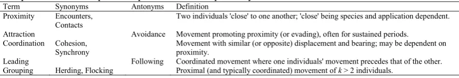
Spatial-temporal interactions can be observed as different spatial-temporal patterns of movement – movement patterns. Here five predominant types of movement patterns relating to spatial-temporal interaction are identified, building from the present movement ecology literature (Table 1). The fundamental movement pattern associated with spatial-temporal interaction is proximity, which occurs when two individuals encounter one another, often termed a contact. Attraction (and the opposite avoidance) represents the time derivative of proximity, specifically movement towards or away from another individual. However in practice the terms attraction and proximity have often been used interchangeably. Coordination represents a second independent movement pattern relating to spatial-temporal interaction. Coordination involves using the temporal sequencing of tracking data in order to model co-occurring movements with similar velocities and headings. Coordination may be considered alongside or independently from proximity in order to understand different aspects of coordinated motion 17_{. Leadership (and} following) represents an important special case of coordinated movement 18_{. Finally, grouping (or herding)} represents the extension of proximity (and often coordinated) movement patterns to k > 2 individuals.

Table 1: Different movement patterns and how they relate to different types of spatial-temporal interaction. The core concept associated with spatial-temporal interaction is proximity.

Term Synonyms Antonyms Definition Proximity Encounters,

Contacts Two individuals 'close' to one another; 'close' being species and application dependent. Attraction Avoidance Movement promoting proximity (or evading), often for sustained periods.

Coordination Cohesion,

Synchrony Movement with similar (or opposite) displacement and bearing; may be dependent on proximity. Leading Following Coordinated movement where one individuals' movement precedes that of the other. Grouping Herding, Flocking Proximal (and typically coordinated) movement of k > 2 individuals.

With different scenarios (e.g., species, age status, time-of-year, habitat) different spatial and temporal patterns in spatial-temporal interaction would be expected. For example, the pattern of spatial-temporal interaction between male and female white-tailed deer will depend on whether or not it is during rut 16_.

3.Methods

Wildilfe tracking data represents a spatial time series; that is a time-series of the spatial locations of the individual being tracked. Tracking data is then stored as a collection of tuples, where each data point contains the information <ID, X, Y, T>, where ID is the individual identifier, X and Y are spatial coordinates (often stored as latitude and longitude) and T is a time-stamp. In the context of analysing spatial-temporal interactions, the nomenclature set-out by 9 _{is used.}

Nomenclature

α or β Individuals of a dyad (telemetry data)

tc Time threshold

dc Distance threshold

Tαβ Temporally simultaneous fixes based on tc

Sαβ Spatially proximal fixes based on dc

STαβ Spatially proximal and temporally simultaneous fixes based on dc and tc

3.1 Spatial-temporal interaction indices

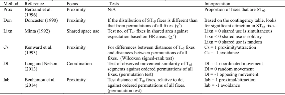
We wish to compare the suite of currently available indices of spatial-temporal interaction, in terms of their ability to identify and different types of interaction, and issues that arise with respect to space, time, and statistical testing. The different methods employed, and how they can be interpreted is shown in Table 3. Prox is a simple measure of the proportion of all fixes that are proximal (i.e., STαβ ) and is used to examine the presence of proximal

movement 19_{. The Doncaster method} 2_{, which is analogous to the Knox test for spatial-temporal interaction} 20_, represents a significant test for proximal (STαβ) behaviour. The Cs index 3 measures the observed separation

distances of Tαβ fixes against expectations derived from the permutations of all fixes, and is analogous to Jacobs

Index 21 _{for spatial-temporal interaction. The Lixn statistic} 4 _{measures counts of T}

αβ fixes in the home range overlap

zone against expectations based on the size of each individual home range and the overlap zone. The DI index 5 measures coordination in the displacement and heading of Tαβ movement segments, where a segment is defined as

the straight-line connecting consecutive fixes. Finally, the Iab statistic 13 _{computes the Bhattacharya coefficient}

between the ‘potential influence domain’ of each Tαβ fix, where the potential influence domain is modelled as a

circular bivariate Gaussian probability density function with σ = dc/2. Statistical tests for both the DI and Iab statistic

follow the ordered permutation system outlined by Benhamou et al. 13_{. The calculation of each index is supported} through the R package wildlifeDI. For a more detailed description of the calculation of each, see the selected reference, or the review by Long et al. 9.

Table 3: Spatial-temporal interaction methods examined in this study.

Method Reference Focus Tests Interpretation

Prox Bertrand et al.

(1996) Proximity N/A Proportion of fixes that are STαβ.

Don Doncaster (1990) Proximity If the distribution of STαβ fixes is different than

that from permutations of all fixes. (χ2₎ Based on the contingency table, looks _{for significant attraction in ST}

αβ fixes. Lixn Minta (1992) Shared space use Test no. of Tαβ fixes in shared area against

expectation based on HR areas. (χ 2₎ Lixn > 0 shared use is simultaneous _{Lixn < 0 shared use is solitary}

Lixn = 0 shared use is random Cs Kenward et al.

(1993) Proximity For differences between distances of Tand distances between permutations of all αβ fixes fixes. (Wilcoxon signed-rank test)

Cs = 1 proximity/attraction Cs = -1 avoidance

DI Long and Nelson (2013)

Coordination Test of observed movement similarity of Tαβ segments against ordered permutations of all fixes. (permutation test)

DI = 1 coordinated movement DI = 0 random movement DI = -1 opposing movement Iab Benhamou et al.

(2014) Proximity Test distance of Tagainst ordered permutations of all fixes. αβ fixes, relative to dc, (permutation test)

Iab = 1 proximal/attraction Iab = -1 avoidance

3.2 Spatial-Temporal Interaction Scenarios

over time. Again, we would expect to see some evidence of significant spatial-temporal interaction. Finally, the fourth scenario represents when we have two individuals engaged in mating behaviour which results in temporal interaction for a consistent extended period. In the fourth scenario, we would expect to see the spatial-temporal interaction clustered in space and time (e.g., associated with the mating location and period). Again, we would expect to see evidence of significant spatial-temporal interaction here.

Table 4: Spatial-temporal interaction scenarios

Scenario Dominant Movement

Pattern Ecological Process Spatial Pattern Time Pattern Statistical Test

Territoriality Random Random NA NA Not significant

Social structure Proximity Behavioural Clustered, patchy Clustered Significant Shared resource use Attraction Landscape Clustered, resource Random Significant

Mating Coordination Behavioural Clustered Clustered Significant

3.3 Simulating Spatial-temporal Interaction

BCRW 22 _{were used to generate synthetic data where two individuals emulate the movement scenarios from} Table 4. In the first scenario, territoriality, each individual moves according to a BCRW, with the biases directed to two disjoint home range centers. The home range centers were chosen so as to emulate territorial behaviour where home range overlap occurs. In the second scenario, social structure, the two individuals move with a BCRW towards a group centroid, which is an independent CRW. In this scenario, individuals randomly switch in and out of social (i.e., biased) phases to mimic real behaviour. In the third scenario, shared resource use, two independent biased random walks are set-up to disjoint home range centroids (as in scenario 1). Individuals randomly switch into and out of resource-driven phases where the bias changes to a shared resource location in between the two home range centers. In scenario 4, the movement of the second individual is biased to that of the first during a prolonged mating period randomly occurring during the motion, otherwise the two individuals move independently.

Each scenario was simulated 100 times to generate a testing dataset upon which to evaluate the six different measures of spatial-temporal interaction. Each measure of spatial-temporal interaction was computed using the associated statistical testing procedures (with the exception of Prox, where we simply identified the value). In all scenarios, a distance threshold of dc = h was used, where h is the input step-length scaling parameter of the BCRW.

A critical level of 0.05 was used to determine statistical significance in all cases. It is expected that identify significant spatial-temporal interaction will occur in the scenarios comprising of social structure, shared resource use, and mating, and no significant spatial-temporal interaction in the territoriality scenario.

In the three scenarios where significant spatial-temporal interaction is expected (i.e., social structure, shared resource use, mating), the level of spatial and temporal clustering of STαβ fixes was evaluated to quantify spatial and

temporal patterns of interaction. Ripley’s K function 23 _{was used to test for spatial clustering in ST}

αβ fixes. The K

function tests if the observed spatial pattern of points deviates significantly from a random spatial pattern. To evaluate temporal clustering a mean nearest-neighbour statistic was used. In this case the nearest neighbour statistic is the time between each STαβ fix and the nearest STαβ fix in time. The mean of the nearest neighbour times is then

tested against a random temporal pattern. Both the spatial and temporal clustering tests require a permutation scheme in which 99 permutations were used. The Ripley’s K and nearest neighbour tests for spatial and temporal clustering were applied to each simulated dyad for each scenario. Expected outcomes for each scenario should follow that from Table 4.

4.Preliminary Results

proximal fixes in the territoriality scenario and the social structure scenario, with the shared resource and mating scenarios exhibiting higher Prox values.

Figure 1: a) The proportion of time in the biased (interactive) phase for simulations from each of 4 scenarios; b) values from Prox analysis, showing the contact rates for simulations from each of 4 scenarios.

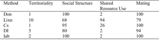
Preliminary results show the variation in ability of different methods for detecting spatial-temporal interaction under different scenarios (Table 5). The Lixn method had the highest rate of false positives, identifying 10/100 of the Territoriality scenario as having significant interaction, while DI had 5. The Lixn method identified only 68/100 of the social structure scenarios as having significant spatial-temporal interaction, while DI returned 80/100. In the shared resource scenario Lixn performed best, identifying 94/100 of the scenarios as having significant spatial-temporal interaction, Cs identified 26/100 as having significant, while the other methods each only identified 2 scenarios. In the mating scenario, Lixn had the lowest success rate, identifying only 79/100, while the other methods had similarly high values.

Table 5: Number of significant results (out of 100 simulations), for each of four scenarios returned for each method employing a statistical test.

Method Territoriality Social Structure Shared

Resource Use Mating

Don 1 100 2 100

Lixn 10 68 94 79

Cs 1 95 26 100

DI 5 80 2 94

Iab 2 100 2 100

Within each type of scenario different patterns of spatial and temporal clustering were expected (Table 4). Spatial clustering was expected in all scenarios, except for territoriality, while temporal clustering was expected only in the social structure and mating scenarios. The preliminary results suggest that spatial clustering of contacts (i.e., proximal fixes based on dc) was present in every simulation (i.e., 100/100). Temporal clustering of contacts

however was observed in no cases for both the territoriality and shared resource scenarios, while 80/100 and 76/100 simulations in the social structure and mating scenarios, respectively.

5.Discussion

clustering was present in some scenarios, and further analysis should investigate the influence of temporal clustering on the presence of Type I or Type II error in different methods.

5.1 Issues of space

To date, few methods have explored mapping spatial-temporal interaction5,24_{. Even the simplest point mapping} techniques, as employed here as the locations of STαβ fixes (i.e., contacts), facilitate new avenues for studying

patterns of spatial-temporal interactions (e.g., through spatial cluster analysis and related methods). One of the most challenging lingering issues in analysing wildlife tracking data is linking observed measures/statistical tests to biologically meaningful behaviours. Spatially explicit analysis of interactive behaviour provides insight into where on the landscape interactions occur. The location of interactive behaviour is important as it can be related to underlying landscape features, which typically relate to biologically meaningful processes, such as searching for limiting resources. Methods capable of relaying explicit spatial location information of interactive behaviour 5,25 _are essential moving forward in order to map spatial-temporal interactions at a finer spatial granularity and link to available remote sensing data.

5.2 Issues of time

Similar to issues of space, few methods have examined temporal trends in spatial-temporal interaction. However, new research has begun to use time-series of spatial-temporal interaction parameters such as DI 5 _{and Prox}26 _{in order} to investigate the timing of interactions. As proposed here, new methods for examining the temporal pattern of interactive behaviour (e.g., clustered vs random in time) may provide useful information for understanding the nature of interactive behaviour occurring in real wildlife systems. For example, temporal patterns of interaction are often directly relatable to seasonal movement behaviours like mating. Linking spatially- and temporally-explicit measures of interaction to dynamic landscape variables (e.g., weather) may provide further insight on the factors influencing spatial-temporal interactions.

5.3 Issues of Statistical Significance

In wildlife movement ecology there has been growing debate over the value of more formal statistical testing versus more exploratory analysis, specifically how to reconcile the differences between statistical and biological significance 27_{. At the forefront of this debate has been the fact that tracking data, especially high resolution GPS} data from modern collars, typically violate underlying assumptions of independence associated with statistical procedures. Due to the serially correlated structure, statistical methods employed in analysis of spatial-temporal interactions are susceptible to both Type I and Type II error, the effects of which change with the resolution of the tracking data. The statistical testing procedure outlined by Benhamou et al.13 _{and employed here for the DI and Iab} statistics uses a wrapping permutation method to maintain the serially correlated structure inherent in the tracking data. Others have explored the use of independent CRWs to generate null distributions for measuring spatial-temporal interaction 11,12_{. However, when the underlying movement process leads to spatial-temporal interactions} that are infrequent or random, statistical testing may miss out on uncovering important interaction behaviour. Such infrequent or random interactions are especially important in the transmission of disease. Similarly, all of these tests are both spatially and temporally global, and thus fail to characterize spatial- and temporal- dynamics in interactive behaviour.

6.Conclusions

interactive behaviour. Finally, statistical testing is difficult due to the problem of generating appropriate null hypotheses. In this case, statistical tests are confounded by the inherent serially correlated structure of movement data. Rare and random bouts of interaction can often be missed when focus is placed on statistical outcomes. Further comparisons of the methods described within are warranted and will be facilitated by the R package wildlifeDI, available freely and openly to other users wishing to study spatial-temporal interactions with their own datasets.

Acknowledgements

The author wishes to thank T. Nelson, S. Webb, and K. Gee, whom all have contributed to the ideas presented herein.

References

1. Macdonald, D. W., Ball, F. G. & Hough, N. G. in A Handb. Biotelemetry Radio Track. (eds. Amlaner, C. J. & Macdonald, D. W.) 405–424 (Pergamon Press, 1980).

2. Doncaster, C. P. Non-parametric estimates of interactions from radio-tracking data. J. Theor. Biol.143, 431–443 (1990).

3. Kenward, R. E., Marcström, V. & Karlbom, M. Post-nestling behaviour in goshawks, Accipiter gentilis: II. Sex differences in sociality and nest-switching. Anim. Behav.46, 371–378 (1993).

4. Minta, S. C. Tests of spatial and temporal interaction amoung animals. Ecol. Appl.2, 178–188 (1992). 5. Long, J. A. & Nelson, T. A. Measuring dynamic interaction in movement data. Trans. GIS17, 62–77 (2013).

6. Böhm, M., Palphramand, K. L., Newton-Cross, G., Hutchings, M. R. & White, P. C. L. Dynamic interactions among badgers: implications for sociality and disease transmission. J. Anim. Ecol.77, 735–745 (2008).

7. Stenhouse, G. B. et al. Grizzly bear associations along the eastern slopes of Alberta. Ursus16, 31–40 (2005).

8. Titcomb, E. M., O’Corry-Crowe, G., Hartel, E. F. & Mazzoil, M. S. Social communities and spatiotemporal dynamics of association patterns in estuarine bottlenose dolphins. Mar. Mammal Sci. In Press (2015). doi:10.1111/mms.12222

9. Long, J. A., Nelson, T. A., Webb, S. L. & Gee, K. L. A critical examination of indices of dynamic interaction for wildlife telemetry studies. J. Anim. Ecol.83, 1216–1233 (2014).

10. Bauman, P. J. The Wind Cave National Park elk herd: home ranges, seasonal movements, and alternative control methods. (1998). 11. White, P. C. L. & Harris, S. Encounters between red foxes (Vulpes vudpes): implications for territory maintenance, social cohesion and

dispersal. J. Anim. Ecol.63, 315–327 (1994).

12. Miller, J. A. Using spatially explicit simulated data to analyze animal interactions: A case study with brown hyenas in Northern Botswana. Trans. GIS16, 271–291 (2012).

13. Benhamou, S., Valeix, M., Chamaillé-Jammes, S., Macdonald, D. W. & Loveridge, A. J. Movement-based analysis of interactions in African lions. Anim. Behav.90, 171–180 (2014).

14. Nathan, R. et al. A movement ecology paradigm for unifying organismal movement research. Proc. Natl. Acad. Sci.105, 19052–19059 (2008).

15. Morgan, E. R., Milner-Gulland, E. J., Torgerson, P. R. & Medley, G. F. Ruminating on complexity: macroparasites of wildlife and livestock. Trends Ecol. Evol.19, 181–188 (2004).

16. Hirth, D. H. Social behavior of white-tailed deer in relation to habitat. Wildl. Monogr.53, 3–55 (1977).

17. Shirabe, T. in GIScience 2006. LNCS, vol. 4197 (eds. Raubal, M., Miller, H. J., Frank, A. U. & Goodchild, M. F.) 4197, 370–382 (Springer-Verlag, 2006).

18. Andersson, M., Gudmundsson, J., Laube, P. & Wolle, T. Reporting leaders and followers among trajectories of moving point objects. Geoinformatica12, 497–528 (2008).

19. Bertrand, M. R., DeNicola, A. J., Beissinger, S. R. & Swihart, R. K. Effects of parturition on home ranges and social affiliations of female white-tailed deer. J. Wildl. Manage.60, 899–909 (1996).

20. Knox, E. G. The detection of space-time interactions. J. R. Stat. Soc. (Series C) Appl. Stat.13, 25–30 (1964).

21. Jacobs, J. Quantitative Measurement of Food Selection : A Modification of the Forage Ratio and Ivlev’s Electivity Index. Oecologia14,

413–417 (1974).

22. Barton, K. a., Phillips, B. L., Morales, J. M. & Travis, J. M. J. The evolution of an ‘intelligent’ dispersal strategy: biased, correlated random walks in patchy landscapes. Oikos118, 309–319 (2009).

23. Ripley, B. D. The second-order analysis of stationary point processes. J. Appl. Probab.13, 255–266 (1976).

24. Buchin, K., Sijben, S., Willems, E. P. & Arseneau, T. J. M. Detecting movement patterns using Brownian bridges. in ACM SIGSPATIAL 119–128 (ACM Press, 2012).

25. Langrock, R. et al. Modelling group dynamic animal movement. Methods Ecol. Evol.5, 190–199 (2014).

26. Schauber, E. M., Nielsen, C. K., Kjaer, L., Anderson, Charles, W. & Storm, D. Social affiliation and contact patterns among white-tailed deer in disparate landscapes: implications for disease transmission. J. Mammal. (2015). doi:10.1093/jmammal/gyu027