Prioritization of combinatorial test cases by incremental interaction coverage

(1)

PRIORITIZATION OF COMBINATORIAL TEST CASES BY

3

INCREMENTAL INTERACTION COVERAGE

4

RUBING HUANG1,∗_{, XIAODONG XIE}2_{, DAVE TOWEY}3_{, TSONG YUEH CHEN}4_, 5

YANSHENG LU1 and JINFU CHEN5

6

1_{School of Computer Science and Technology, Huazhong University of Science and Technology} 7

Wuhan, Hubei 430074, P.R. China

8

2_{School of Computer Science and Technology, Huaqiao University} 9

Xiamen, Fujian 362021, P.R. China

10

3_{BNU-HKBU: United International College, Zhuhai, Guangdong 519085, P.R. China} 11

4_{Faculty of Information and Communication Technologies, Swinburne University of Technology} 12

Hawthorn, Victoria 3122, Australia

13

5_{School of Computer Science and Telecommunication Engineering, Jiangsu University} 14

Zhenjiang, Jiangsu 212013, P.R. China

15

Combinatorial testing is a well-recognized testing method, and has been widely applied

16

in practice. To facilitate analysis, a common approach is to assume that all test cases

17

in a combinatorial test suitehavethe same fault detection capability. However, when

18

testing resources are limited, the order of executing the test cases is critical. To improve

19

testing cost-effectiveness, prioritization of combinatorial test cases isemployed. The most

20

popular approach is based on interaction coverage, which prioritizes combinatorial test

21

cases by repeatedly choosingan unexecuted test case that covers the largest number of

22

uncoveredparameter value combinations of a given strength (level of interaction among

23

parameters). However, this approach suffers from some drawbacks. Based on previous

24

observations that the majority of faults in practical systems canusuallybe triggeredwith

25

parameter interactions of small strengths, we propose anewstrategy of prioritizing

com-26

binatorial test cases by incrementally adjusting the strength values. Experimental results

27

show that our method performs better thantherandom prioritization technique and the

28

technique of prioritizing combinatorial testsuitesaccording to test case generation

or-29

der, and has better performance thantheinteraction-coverage-based test prioritization

30

technique in mostcases.

31

Keywords: Software testing; combinatorial testing; test case prioritization; interaction

32

coverage; incremental interaction coverage; algorithm.

33

1. Introduction

34

Suppose that a system under test (SUT) is affected by itskparameters (or factors),

35

and each of these parameters may have many possible values (or levels). Ideally,to

36

ensure system quality, we should test all combinations of parameter values. However,

37

it is practically infeasible todo this due to the large amount of resources and effort

38

∗_{Corresponding Author: School of Computer Science and Technology, Huazhong University of}

Science and Technology, Wuhan, Hubei 430074, China. Email: [email protected].

(2)

required, especially for complex systems with a large number of parameters and

1

values.

2

Combinatorial testing (or combinatorial interaction testing), a black-box

test-3

ing technique, aims at generating an effective test suite in order to detect failures

4

triggered by the interactions among parameters of the SUT. It is widely applied in

5

various applications, especially for highly-configurable systems [1–5]. Combinatorial

6

testingprovides a tradeoff between testing effectiveness and efficiency, as it uses a

7

smaller test suite that covers certain key combinations of parameter values for

sam-8

pling the entire combination space. For example, 2-wise combinatorial testing (or

9

pairwise testing where the level of interaction among parameters, the strength, is

10

2) only requires the generated test suite to cover all possible 2-tuples of parameter

11

values (referred to as 2-wise parameter value combinations).

12

In the faultmodel of combinatorial testing, it is assumed that failures are caused

13

by parameter interactions. Previous studies have shown that faults can normally

14

be identified by testing interactions among a small number of parameters [1, 6, 7].

15

A failure-causing interaction is called a faulty interaction, and the size of a faulty

16

interaction (that is, the number of parameters required to detect a failure) is referred

17

to as thefailure-triggering fault interaction (or FTFI) number [1, 6].

18

Traditionally, combinatorial testing treats all test cases equally in a test suite.

19

However, the order of executing the test cases may be critical in practice, for example

20

in regression testing with limited test resources. Therefore, the potentially

failure-21

revealing test cases should be executed as early as possible. In other words, a

well-22

designedtest case execution order may be ableto identify failures earlier, and thus

23

enable earlier fault characterization, diagnosis and revision[7]. To improve testing

24

efficiency, test case prioritization [8], which means to prioritize test cases according

25

tosome strategy, has beenintroduced. In test case prioritization, a prioritized test

26

suite is generally referred to as a test sequence.

27

Test case prioritization of combinatorial test suites has also been well

stud-28

ied [4, 9–15]. Many techniques have been proposed to guide the prioritization of

29

combinatorial test cases, such as random prioritization [9] and

branch-coverage-30

based prioritization [13]. The most well-studied approach of prioritizing

combina-31

torial test suite is based on interaction coverage (called interaction-coverage-based

32

prioritization), which prioritizes test cases by repeatedly selecting an unexecuted

33

element suchthat it covers the largest number of uncovered parameter value

com-34

binations of a given strength [4, 9–15].

35

However, the interaction-coverage-based prioritization technique has two

chal-36

lenges. Firstly, given a combinatorial test suite T of strength t, the prioritization

37

method by interaction coverage only takes account of parameter value combinations

38

of strengthtfor orderingT, which means that a test sequence prioritized by

inter-39

action coverage may only favor parameter value combinations of strengtht. In other

40

words, this test sequence may not be effective forτ-wise (1≤τ < t) combinations

41

of parametric values. A second challenge is thattesters need to specify the strength.

42

Kuhn and his colleagues [1, 6] investigated interaction failures by analyzing the

(3)

faultreports of several software projects. They concluded that over 50% of faults can

1

be triggered by one-wiseinteractions; more than 70% of faults can be detected by

2

testing two-wise interactions; and approximately 90% of the faults can be discovered

3

with three-wise interactions. In other words, the majority of faults in the SUT

4

are generally caused by interactions of small strengths. Therefore, it is reasonable

5

and practical to prioritize combinatorial test cases by covering all parameter value

6

combinations at small strengths as early as possible. /*** Dave’s comment [1]:

7

perhaps delete the next sentence ***/ We would like to emphasize this category of

8

failures in this paper.

9

Motivated by these facts, we propose a novel technique of prioritizing

combina-10

torial test cases based on incremental interaction coverage, which orders

combina-11

torial test cases by reusing already selected test cases and incrementally adjusting

12

the strength values. Given a combinatorial test suite T of strengtht, our strategy

13

aims to prioritize T into a test sequence such that all possible parameter value

14

combinations of each strength lower thant would be covered as earlyas possible.

15

Therefore, our method has at least two advantages over the

interaction-coverage-16

based prioritization technique: (1) no selection of strength is required in advance;

17

and (2) different strengths are considered. Compared with the

interaction-coverage-18

based prioritization technique, our method provides a priority of strengths lower

19

than t over the strength t. In other words, our prioritized test suites cover all

t-20

wise combinations of parameter values with lower priorities – not just all parameter

21

value combinations at strengths lower thant.In terms of covering parameter value

22

combinations and fault detection, experimental results show that our method has

23

better performance than the random prioritization approach and the method of

pri-24

oritizing combinatorial test suite according to the test case generation order, and

25

also performs better than the interaction-coverage-based prioritization technique in

26

most cases.

27

This paper is organized as follows. Section 2 introduces some preliminaries about

28

combinatorial testing, and test case prioritization. Section 3introducesa new

prior-29

itization strategy based on incremental interaction coverage, and analyzes its time

30

complexity. Section 4 presents results ofthesimulations and empirical studies.

Sec-31

tion 5 summarizes some related work, and Section 6 describes the conclusions and

32

potential future work.

33

2. Preliminaries

34

In this section, some preliminaries of combinatorial testing and test case

prioritiza-35

tion are presented.

36

2.1. Combinatorial testing 37

Combinatorial testing is widely used in the combinatorial test space to generate an

38

effective test suite for detecting interaction faults that are triggered by interactions

39

among parameters in the SUT.

(4)

Suppose that the SUT has k parameters P1, P2,· · ·, Pk, which may represent

1

user inputs or configuration parameters, and each parameter Pi has discrete valid

2

values from the finite set Vi. Let C be the set of constraints on parameter value

3

combinations, andR be the set of interaction relations among parameters. In the

4

remainder of this paper, we will refer to acombination of parameters as aparameter 5

combination, and acombination of parameter valuesor aparameter value combina-6

tion as avalue combination.

7

Definition 1. A test profile, denoted as T P(k,|V1||V2| · · · |Vk|, C), is about the

8

information on a combinatorial test space of the SUT, including k parameters,

9

|Vi|(i= 1,2,· · · , k) values for thei-th parameter, and constraintsC on value

com-10

binations.

11

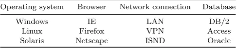
For example, Table 1 gives the configurations of a component-based system,

12

in which there are four configuration parameters, each of which has three values.

13

Therefore, its test profile can be written asT P(4,34_,_∅).

14

Definition 2.Given a test profile denoted byT P(k,|V1||V2| · · · |Vk|, C), ak-tuple

15

(v1, v2,· · ·, vk) is a test case for SUT, wherevi ∈Vi(i= 1,2,· · · , k).

16

For example, a 4-tuple tc = (Windows,IE,LAN,Access) is a test case for the

17

SUT shown in Table 1.

18

Definition 3.Given aT P(k,|V1||V2| · · · |Vk|, C), anN×kmatrix is at-wise (1≤

19

t ≤ k) covering array denoted as CA(N;t, k,|V1||V2| · · · |Vk|), which satisfies the

20

following properties: (1) each columni(i= 1,2,· · ·, k) contains only elements from

21

the setVi; and (2) the rows of eachN×tsub-matrix cover allt-tuples of parametric

22

values from thetcolumns at least once.

23

When |V1|= |V2| =· · · =|Vk| =v, the covering array can also be written as

[image:4.595.183.427.514.564.2]

24

Table 1. Configurations of a component-based system.

Operating system Browser Network connection Database

Windows IE LAN DB/2

Linux Firefox VPN Access

Solaris Netscape ISND Oracle

Table 2. A combinatorial test suite for pairwise testing.

Test No. Operating system Browser Network connection Database

1 Windows IE LAN DB/2

2 Windows Firefox VPN Oracle

3 Windows Netscape ISND Access

4 Linux IE ISND Oracle

5 Linux Firefox LAN Access

6 Linux Netscape VPN DB/2

7 Solaris IE VPN Access

8 Solaris Firefox ISND DB/2

[image:4.595.161.448.606.716.2]

(5)

CA(N;t, k, v). Obviously, the interaction relation set R has elements of the same

1

size forCA(N;t, k,|V1||V2| · · · |Vk|), that is,R={{Pj₁, Pj₂,· · ·, Pj_t}|1≤j1< j2<

2

· · ·< jt≤k, tis fixed} and|R|=Ct k.

3

On the other hand, a covering arrayT denoted asCA(N;t, k,|V1||V2| · · · |Vk|) is

4

also a covering array of strengthτ(1≤τ < t). In other words,T can also be written

5

asCA(N;τ, k,|V1||V2| · · · |Vk|) where 1≤τ < t. Thus, there exists a subsetT0⊆T

6

such thatT0 is a covering array of strengthτ, that is,CA(|T0_{|, τ, k,}_{|V1||V2| · · · |Vk|).}

7

For example, to achieve exhaustive testing of all possible value combinations

8

for the system shown in Table 1, we should require 34 = 81 test cases. However,

9

as shown in Table 2, 2-wise combinatorial testing requires only a set of 9 test

10

cases (denoted asCA(9; 2,4,34_{) or}_{CA(9; 2,}_4,_{3)) for covering all pairs of parameter}

11

values.

12

Definition 4.Given aT P(k,|V1||V2| · · · |Vk|, C), a variable-strength covering array,

13

denoted asV CA(N;t, k,|V1||V2| · · · |Vk|, Q), is anN×kcovering array of strength

14

tcontainingQ, which is a set of CAs, every element of which is of strength> tand

15

is defined on a subset ofkparameters.

16

Intuitively speaking, aV CA(N;t, k,|V1||V2| · · · |Vk|, R) can also be considered a

17

CA(N;t, k,|V1||V2| · · · |Vk|), with the interaction relation setRof the VCA

contain-18

ing elements of different sizes, that is, the VCA contains other CAs.

19

Each row of a covering array or variable-strength covering array stands for a

20

test case while each column represents a parameter of the SUT. Testing with a

21

t-wise covering array is called t-wise combinatorial testing, while testing with a

22

variable-strength covering array is called variable-strength combinatorial testing.

23

In combinatorial testing, the uncovered t-wise value combinations distance

24

(UVCD) is a distance measure often used to evaluate test cases when constructing

25

a covering array or variable-strength covering array [16].

26

Definition 5. Given a combinatorial test suite T, strength t, and a test case tc,

27

uncoveredt-wise value combinations distance (UVCD) oftcis defined as:

28

U V CDt(tc, T) =|CombSett(tc)\CombSett(T)|, (1) where CombSett(tc) is defined as the set of t-wise value combinations covered by

29

test casetc, whileCombSett(T) is the set oft-wise value combinations covered by

30

test suiteT. More specifically, lettc= (v1, v2,· · ·, vk) wherevi∈Vi(i= 1,2,· · · , k),

31

CombSett(tc) andCombSett(T) can be respectively written as follows:

32

CombSett(tc) ={(vj1, vj2,· · ·, vjt)|vj1 ∈Vj1, vj2 ∈Vj2,· · ·, vjt ∈Vjt,

1≤j1< j2<· · ·< jt≤k}, (2)

CombSett(T) = [ tc∈T

(6)

To reduce the cost of combinatorial testing, many researchers have focused on

al-1

gorithms to generate the optimal combinatorial test suite with the minimal number

2

of test cases. Unfortunately, it has beenproven that the problem of constructing

cov-3

ering arrays or variable-strength covering arraysis NP-Complete [17].Nevertheless,

4

many strategies and tools for building combinatorial test suiteshave been developed

5

in recent years. Some major approaches to combinatorial test suite construction

6

involve greedy algorithms, heuristic search algorithms, recursive algorithms, and

7

algebraic methods(see [7] for more details).

8

2.2. Test case prioritization 9

To illustrate our work clearly, let us initially define a few terms. /*** Dave’s

10

comment [2]: Earlier, we used tc to refer to test cases, should we continue that

11

here? ***/ Suppose T = {t1, t2,· · ·, tN} is a test suite of size N, and S =

12

hs1, s2,· · ·, sNi is an ordered set suite (we call it a test sequence) where si ∈ T

13

andsi 6=sj(i, j= 1,2,· · · , N;i6=j). If two test sequences areS1=hs1, s2,· · · , smi

14

and S2 = hq1, q2,· · · , qni, we define S1ZS2 as hs1, s2,· · ·, sm, q1, q2,· · ·, qni. By 15

definition,T\S is the maximal subset ofT whoseelements are not inS.

16

Test case prioritization is done to obtain a schedule of test cases, sothat,

accord-17

ing to some criteria (such as the cost of test case execution or statement coverage),

18

test cases with higher priorityare executed earlier in testing. A well-prioritized test

19

sequence may improve the likelihood of detecting faults early. The problem of test

20

case prioritization is defined asfollows, from [8].

21

Definition 5. Given (T,Ω, f), whereT is a test suite, Ω is the set of all possible

22

test sequences obtained by ordering test cases of T, and f is a function from Ω to

23

theset ofreal numbers, the problem of test case prioritization is to findanS∈Ω

24

such that:

25

(∀S0) (S0∈Ω) (S06=S) [f(S)≥f(S0)]. (4) In Equation 4,f is a function which evaluates a test sequence S by returning

26

an award value. /*** Dave’s comment [3]: please confirm the following sentence is

27

correct ***/ The most well-known function isa weighted average of the percentage

28

of faults detected (APFD)[18], which is a measure of how quickly a test sequence

29

can detect faults during the execution. LetT be a test suite of sizen, and letF be

30

a set ofm faults revealed by T. Let SFi be the first test case in test sequence S

31

ofT which detects faulti. The APFD for test sequenceSis given by the following

32

equation from [18]:

33

AP F D= 1−SF1+SF2+· · ·+SFm

n×m +

1

2n. (5)

To date, many techniques of test case prioritization have been proposed

ac-34

cording to different criteria, such as time-aware prioritization [19], search-based

(7)

prioritization [20], risk-exposure-based prioritization [21], source-code-based

priori-1

tization [8, 22], fault-severity-based prioritization [23],and history-based

prioritiza-2

tion [24]. Most test case prioritization strategies can be categorized into two classes:

3

greedy methods and meta-heuristic search methods [15].

4

3. Incremental-Interaction-Coverage-Based Test Prioritization

5

In this section, we present a method of prioritizing combinatorial test cases based

6

on incremental interaction coverage (denoted IICBP), a heuristic algorithm

imple-7

menting this method, and a complexity analysis ofthealgorithm.

8

3.1. Method 9

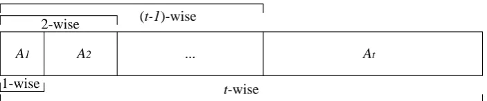
The IICBP technique divides a CA(N;t, k|V1||V2| · · · |Vk|) intot independent

sub-10

sets (A1, A2,· · · , At) such that:

11

Ai\Aj=∅, i, j= 1,2,· · · , t, i6=j; (6)

j

[

i=1

Ai=CA( j

X

i=1

|Ai|;j, k,|V1||V2| · · · |Vk|), j= 1,2,· · · , t, (7) whereAi(i= 1,2,· · ·, t) is a test sequence prioritized by interaction-coverage-based

12

strategy [4, 11–13, 15] of strengthi. Each subsetAj (j = 2,3,· · · , t) is prioritized

13

by ICBP using the seeding setSj−1

l=1Al. However, the processes of covering array

14

partition and prioritization for each sub-partition are inter-related in such a way

15

that once a subpartition is completed, test case prioritization of this sub-partition

16

is also completed. In other words, each test case in Ai(i = 1,2,· · · , t) is selected

17

by using strengthiand previously chosen test cases as seeds. Once alli-wise value

18

combinations are covered by the selected test cases (that is,Aihas been successfully

19

constructed), strengthiis incremented by 1. The criterion is to choose the element

20

e0 from test suiteT as the next test element in test sequenceS such that:

21

(∀e) (e∈T) (e6=e0) [U V CDi(e0, S)≥U V CDi(e, S)]. (8)

A1 A2 ... At

t-wise 2-wise

1-wise

[image:7.595.134.486.607.680.2]

(t-1)-wise

(8)

Algorithm 1Select the best test element (BTES)

Input: Already prioritized test setS, candidate test suite T, and strength t

Output: Best test elementbest data∈T

1: Setbest distance=−1; 2: for(each elemente∈T)

3: Calculate UVCD ofe, that is,U V CDt(e, S); 4: if (U V CDt(e, S)≥best distance)

5: best distance=U V CDt(e, S); 6: best data=e;

7: end if

8: end for

9: return best data.

Algorithm 2Interaction-coverage-based prioritization of combinatorial test cases

(ICBP)

Input: Covering arrayCA(N;t, k,|V1||V2| · · · |Vk|), denoted asT

Output: Test sequenceS

1: InitializeS=hi;

2: while (|S| 6=N)

3: best data=BT ES(S, T, t); //Generate the best test element. 4: T =T\ {best data};

5: S =S_Zhbest datai;

6: end while

7: return S.

Algorithm 3 Incremental-interaction-coverage-based prioritization of

combinato-rial test cases (IICBP)

Input: Covering arrayCA(N;t, k,|V1||V2| · · · |Vk|), denoted asT

Output: Test sequenceS

1: InitializeS=hi,τ= 1, T0=T;

2: while (|S| 6=N)

3: if (|CombSetτ(S)|==|CombSetτ(T)|) 4: τ =τ+ 1;

5: end if

6: best data=BT ES(S, T0, τ); //Generate the best test element. 7: T0 =T0\ {best data};

8: S =S_Zhbest datai;

9: end while

(9)

The process is repeated until all Ai(i = 1,2,· · ·, t) are prioritized according to

1

i-wise interaction coverage. Fig. 1 gives a schematic diagram for the relationship

2

betweenAi and the relevanti-wise interaction coverage.

3

Since the element selection criterion (see Equation 8) is widely used in the

4

prioritization of combinatorial test cases, we present the algorithm implementing

5

this criterion (Algorithm 1). However, there may exist more than one best test

6

element, indicating that they have the same maximal UVCD value. In such a tie

7

case, we randomly select one best element. The test case prioritization technique

8

by interaction coverage (denoted as ICBP) [4, 11–13, 15]is also given in Algorithm

9

2, and Algorithm 3 presents the detailed IICBP processes.

10

In this paper, we assume that a combinatorial test suite is equivalent to a

11

covering array, and that all parameters are independent. In other words, the

12

variable-strength covering array is not considered in this paper. Also, constraints

13

on value combinations are ignored. Therefore, the test profile can be abbreviated

14

asT P(k,|V1||V2| · · · |Vk|).

15

3.2. Complexity analysis 16

In this subsection, we briefly analyze the time complexity for the IICBP algorithm

17

(Algorithm 3). Given a CA(N;t, k,|V1||V2| · · · |Vk|), denoted as T, we define a =

18

max1≤i≤k{|Vi|}. /*** Dave’s comment [4]: is there any reason for choosing ‘a‘?

19

Can we give an explanation? ***/

20

We first analyze the time complexity of selecting the i-th (i= 1,2,· · ·, N) test

21

case, which depends on two factors: (1) the number of candidates required for the

22

calculation of UVCD; and (2) the time complexity of calculating UCVD of strength

23

l (1≤l≤t) for each candidate during the process of constructingAl.

24

For (1), it requires (N−i)+1 test cases to compute UVCD. For (2), according to Cl

k l-wise parameter combinations, we divide all possiblel-wise value combinations that are derived from aT P(k,|V1||V2| · · · |Vk|) intoCkl sets that form

Πl={πl|πl={(vi₁, vi₂,· · ·, vi_l)|vi_j ∈Vi_j, j= 1,2,· · · , l},

1≤i1< i2<· · ·< il≤k}. (9) As a consequence, when using a binary search, the order of time complexity of

25

(2) isO(P

πl∈Πllog(|πl\CombSetl(T)|)), which equalsO(

P

πl∈Πllog(|πl|)). Let us

26

define the following function:

27

fl=







0, ifl= 0; l

P

i=1

|Al|,if 1≤l≤t. (10)

FromEquation 10, we haveft=Pt

l=1|Al|=N.

28

According to Al(1 ≤ l ≤ t), the order of time complexity of constructing Al isO((Pfl

i=fl−1+1(N−i+ 1))×(

P

(10)

are included in the algorithm IICBP execution, the order of time complexity can be described as follows:

O(IICBP) =O( t

X

l=1 ((

fl

X

i=fl−1+1

(N−i+ 1))×( X πl∈Πl

log(|πl|))))

< O( t

X

l=1 ((

fl

X

i=fl−1+1

(N−i+ 1))×(Ckl ×log(al))))(1≤l≤t). (11)

There exists an integerµ(1≤µ≤t) such that:

1

(∀l) (1≤l≤t) (µ6=l) [(C_kµ×log(aµ))≥(Ckl×log(a l

))]. (12)

As a consequence,

O(IICBP)< O( t

X

l=1 ((

fl

X

i=fl−1+1

(N−i+ 1))×(C_kµ×log(aµ))))

=O(( N

X

i=1

(N−i+ 1))×(C_kµ×log(aµ)))

=O(C_kµ×log(aµ)×(N2+N)/2). (13) Therefore, we can conclude that the order of time complexity of algorithm IICBP

2

isO(N2×C_kµ×log(aµ))(1≤µ≤t).a

3

As discussed in [15], the order of time complexity of algorithm ICBP (Algorithm

4

2) is O(N2×C_kt×log(at)). /*** Dave’s comment [5]: please confirm the next

5

sentence ***/ According to Appendix A, if 1≤t <dk

2e,µ=t, or ifd

k

2e ≤t≤k, 6

µ=dk

2e, then the order of time complexity of algorithm IICBP is the same as that 7

of algorithm ICBP.

8

4. Experimental Results

9

In this section, some experimentalresults from simulations and experiments with

10

real programsare presented to analyze the effectiveness of the prioritization of

com-11

binatorial test cases by incremental interaction coverage.We evaluatetest sequences

12

prioritized by algorithm IICBP (denotedIICBP) by comparing with those ordered

13

by three other strategies: (1) test sequence according to covering array generation

14

sequence (denotedOriginal); (2) random test sequence whose ordering is randomly

15

prioritized (denotedRandom); and (3) test sequence prioritized by algorithm ICBP

16

(denotedICBP).

17

a_{If 1}_≤_{t <}_dk

2e,µ=t; ifd k

2e ≤t≤k,µ=d k

(11)

[image:11.595.125.480.185.257.2]

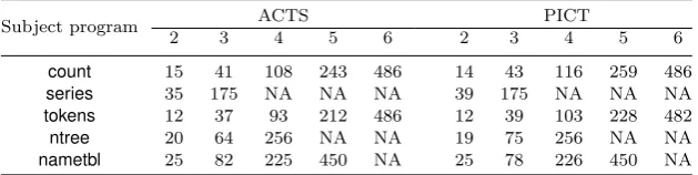
Table 3. Sizes of covering arrays for four test profiles.

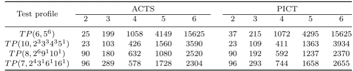
Test profile ACTS PICT

2 3 4 5 6 2 3 4 5 6

T P(6,56₎ ₂₅ ₁₉₉ ₁₀₅₈ ₄₁₄₉ ₁₅₆₂₅ ₃₇ ₂₁₅ ₁₀₇₂ ₄₂₉₅ ₁₅₆₂₅

T P(10,23₃3₄3₅1₎ ₂₃ ₁₀₃ ₄₂₆ ₁₅₆₀ ₃₅₉₀ ₂₃ ₁₀₉ ₄₁₁ ₁₃₆₃ ₃₉₃₄

T P(8,26₉1₁₀1₎ ₉₀ ₁₈₀ ₆₃₂ ₁₀₈₀ ₂₅₂₀ ₉₀ ₁₉₂ ₅₉₂ ₁₂₃₇ ₂₃₇₀

T P(7,24₃1₆1₁₆1₎ ₉₆ ₂₈₉ ₅₇₈ ₁₇₂₈ ₂₃₀₄ ₉₆ ₂₉₃ ₇₄₄ ₁₆₅₈ ₂₆₅₅

4.1. Simulations 1

We initially designed some typical test profiles to construct covering arrays, then

2

applied different test case prioritization techniques to prioritize them, evaluating

3

each prioritization strategy Three simulations wereinvolved. The first simulation

4

was to evaluate the rate of value combinations covered by the different

prioriti-5

zation techniques. The second and third simulations aimed at assessing rates of

6

fault detection for different test sequences when executingall, or some test cases,

7

respectively.

8

4.1.1. Simulation instrumentation 9

We designedfour test profiles as four system models with details shown in Table

10

3. The first two test profiles wereT P(6,56_{) and}_{T P}_(10,₂3₃3₄3₅1_{), both of which}

11

have been used in previous studies [15]. The third and fourth test profiles (that

12

is,T P(8,26₉1₁₀1_{) and}_{T P}_(7,₂4₃1₆1₁₆1₎₎_were_{from real-world}_{applications: a real}

13

configuration model of GNUzip (gzip);and a module of a lexical analyzer system

14

(flex).

15

The original covering arrays were generated by two different tools: Advanced 16

Combinatorial Testing System (ACTS) [25, 26] and Pairwise Independent Combi-17

natorial Testing (PICT) [27]. Both of these are supported by greedy algorithms,

18

and implemented, respectively, bytheIn-Parameter-Order (IPO) method [25] and

19

the one-test-at-a-time approach (generating one test case each time) [28]. We

fo-20

cusedon covering arrays with strengtht= 2,3,4,5,6; and the sizes of the covering

21

arrays generated by ACTS or PICT are given in Table 3. Since randomization is

22

used in some test case prioritization techniques, weraneach test profile 100 times

23

and report the average of the results.

24

4.1.2. Simulation One: Rate of covering value combinations 25

In this simulation, wemeasuredhow quickly a test sequencecouldcover value

com-26

binations of different strengths. We onlyconsidered strengtht= 2,3,4.Algorithm

27

ICBP requires that the strength t be initialized in advance. However, because we

28

sometimes may not know the strength of a covering array in practical testing

ap-29

plications, we also take account of test sequences ordered by algorithm ICBP when

30

selecting lower strengthτ(1< τ < t), that is,ICBPτ.

(12)

1. Metrics:Average percentage of combinatorial coverage(APCC) [15] is used as the

1

metric to evaluate the rate of value combinations covered by a test sequence. The

2

APCC values range from 0% to 100%; higher APCC values mean better rates

3

of covering value combinations. Let a test sequence be S = hs1, s2,· · · , sNi,

4

obtained by prioritizing aCA(N;t, k,|V1||V2| · · · |Vk|), the formulaforAPCC at

5

strengthτ is given as follows:

6

AP CCτ(S) =

PN−1

i=1 |

Si

j=1CombSetτ(sj)|

N× |CombSetτ(Tall)| , (14) whereTall is the set of all test cases fromT P(k,|V1||V2| · · · |Vk|).

7

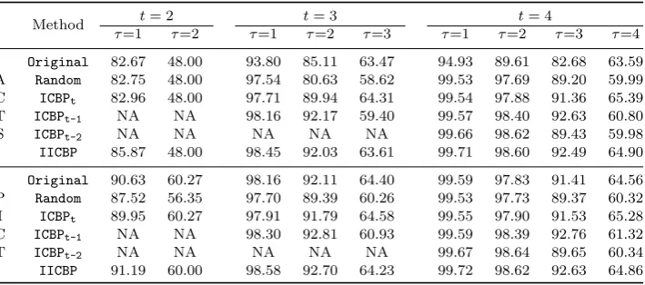
2. Results and analysis: For covering arrays of strengtht(2≤t≤4) on individual

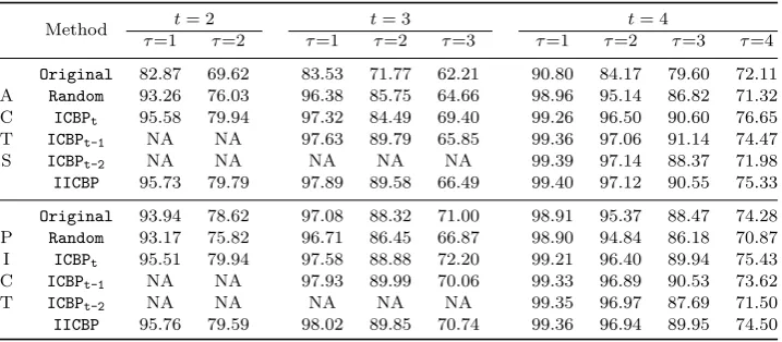
[image:12.595.129.484.361.518.2]

8

Table 4.AP CCτ metric (%) for different prioritization techniques forT P(6,56).

Method t= 2 t= 3 t= 4

τ=1 τ=2 τ=1 τ=2 τ=3 τ=1 τ=2 τ=3 τ=4

Original 82.67 48.00 93.80 85.11 63.47 94.93 89.61 82.68 63.59 A Random 82.75 48.00 97.54 80.63 58.62 99.53 97.69 89.20 59.99 C ICBPt 82.96 48.00 97.71 89.94 64.31 99.54 97.88 91.36 65.39 T ICBPt-1 NA NA 98.16 92.17 59.40 99.57 98.40 92.63 60.80

S ICBPt-2 NA NA NA NA NA 99.66 98.62 89.43 59.98

IICBP 85.87 48.00 98.45 92.03 63.61 99.71 98.60 92.49 64.90

Original 90.63 60.27 98.16 92.11 64.40 99.59 97.83 91.41 64.56 P Random 87.52 56.35 97.70 89.39 60.26 99.53 97.73 89.37 60.32 I ICBPt 89.95 60.27 97.91 91.79 64.58 99.55 97.90 91.53 65.28 C ICBPt-1 NA NA 98.30 92.81 60.93 99.59 98.39 92.76 61.32

T ICBPt-2 NA NA NA NA NA 99.67 98.64 89.65 60.34

IICBP 91.19 60.00 98.58 92.70 64.23 99.72 98.62 92.63 64.86

τ=1 τ=2 τ=1 τ=2 τ=3 τ=1 τ=2 τ=3 τ=4

IICBP 89.31 66.90 97.73 92.06 74.15 99.47 98.15 93.61 79.38

[image:12.595.128.486.560.717.2]

(13)

[image:13.595.126.485.187.344.2]

τ=1 τ=2 τ=1 τ=2 τ=3 τ=1 τ=2 τ=3 τ=4

IICBP 95.73 79.79 97.89 89.58 66.49 99.40 97.12 90.55 75.33

[image:13.595.125.485.389.545.2]

IICBP 95.76 79.59 98.02 89.85 70.74 99.36 96.94 89.95 74.50

τ=1 τ=2 τ=1 τ=2 τ=3 τ=1 τ=2 τ=3 τ=4

IICBP 94.47 75.01 98.16 91.86 72.42 99.08 96.02 85.63 62.62

IICBP 94.47 75.66 98.18 91.87 73.74 99.28 96.87 89.12 71.22

test profiles, we have the following observationsbased on the results reportedin

1

Tables 4–6. Each table corresponds to a particular test profile.

2

(a) Combinatorial test sequences prioritized by IICBP strategy have greater

3

APCCτ(1≤τ ≤t) valuesthanOriginaltest sequences andRandomtest

se-4

quences. Therefore, theIICBPtechnique outperformsOriginalandRandom.

5

(b) Given a covering array of strengtht, theICBPτhas the highest APCCτwhen

6

1< τ ≤t; but theIICBPhas the highest APCCτ0 when 1≤τ06=τ ≤t.

7

(c) The ACTS Original test sequences often have lower APCC values than

8

Randomtest sequences; the PICTOriginaltest sequences always outperform

9

Randomtest sequences, and occasionally outperformICBPt-1andICBPt-2test

10

sequences.

(14)

Observation (a) is easily explained, hence, we just explain the second and the

1

third observations here. For observation (b), since ICBP prioritizes combinatorial

2

test cases by using strengthτ, therefore its APCC value is the highest at strength

3

τ. However,IICBPcomprehensively considers different strengths for prioritizing test

4

cases, and hence it has the highest APCC values at other strength values.

5

For observation (c), the difference in performance is due to the different

mecha-6

nisms involved in implementing ACTS and PICT. For example, without loss of

gen-7

erality, suppose we have aT P(k,|V1||V2| · · · |Vk|) with|V1| ≥ |V2| ≥ · · · ≥ |Vk|. The

8

ACTS algorithm first useshorizontal growth[25,26] to build at-wise (2≤t≤k) test

9

set for the firsttparameters. This implies that it needs at least 1+(|V1|−1)Qt

i=2|Vi|

10

test casesto coverall 1-wise value combinations. On the other hand, PICT selects

11

a next test case such that it covers the largest number oft-wise value combinations

12

that have not been covered – amechanism similar to that of ICBP.

13

In summary, given a covering array of strengtht,IICBPstrategyperformsbetter

14

than Original and Random strategies with respect to APCCτ(1 ≤ τ ≤ t), and

15

performs better than ICBP technique of strength τ in for strengths that are not

16

equal toτ.

17

4.1.3. Simulation Two: Rate of fault detection when executing all test cases 18

In the second simulation, we modeled four systems with a number of failures by

19

using the same four test profiles as in Section 4.1.1 to analyze the fault detection

20

rate of each prioritization technique when executing all test cases in a covering

21

array.

22

With regard to the distribution of failures, we assigned some failures at lower

23

strengths accordingto resultsreported in [1,6]. For example, in [1], several software

24

projectswere studied and the interaction faults were reported to have 29% to 82%

25

faults as 1-wise faults (that is, the FTFI number is 1); 6% to 47% of faults as

26

2-wise faults; 2% to 19% as 3-wise; 1% to 7% of faults as 4-wise; and even fewer

27

faults beyond 4-wise interactions. Therefore, in our simulation we only considered

28

simulated interaction faults of the FTFI number = 1,2,3,4. As a result, the fault

29

distribution simulated for each test profile was designed as following: thirty 1-wise

30

interaction faults; forty 2-wise interaction faults; twenty 3-wise interaction faults;

31

and five 4-wise interaction faults. Each injected fault was randomly generated with

32

replacement in individual test profiles. Since the simulated interaction fault was

33

randomly chosen and some prioritization strategies involved some randomization,

34

we ran each algorithm 100 times for each test profile, and report the average of the

35

results.

36

1. Metrics: The APFD metric [18]is often used to evaluate fault detection rates of

37

different prioritization techniques. However, this metric does have a requirement

38

that all faults should be detected by a given test sequence. In other words, if a

39

fault cannot be detected, the APFD metric fails. Thenormalized APFD metric

(15)

(NAPFD) [13] has been proposed as an enhancement of APFD. It includes

infor-1

mation about both fault finding and time of detection. The higher the NAPFD

2

value, the higher the fault detection rate. Similar to the definition of APFD

3

given in Equation 5, the formula for NAPFD is presented as follows:

4

N AP F D=p−SF1+SF2+· · ·+SFm

n×m +

p

2n, (15)

wherem,n, andSFi(i= 1,2,· · ·, m) have the same interpretations as in APFD,

5

andprepresents the ratio of the number of faults identified by selected test cases

6

relative to the number of faults detected by the full test suite. If a fault,fi, is

7

never found, we set SFi = 0. Obviously, if all faults can be detected, NAPFD

8

and APFD are identical due top= 1.0.

9

2. Results and analysis: Fig. 2 presents the simulation results in terms of the

10

NAPFD metric values for different prioritization techniques, based on which

11

we have the following observations.

12

(a) The IICBPtechnique has significantly better fault detection rates than the

13

ACTS Original method, but only slightly better performance than the

14

PICT Originalmethod.

15

(b) TheIICBP test sequences have higherNAPFD valuesthan theRandomtest

16

sequences.

17

(c) Compared to ICBP, IICBP has similar NAPFD values. More specifically,

18

when prioritizing the covering arrays of strength t = 2, the IICBP

failure-19

detection rate is sometimes slightly less than that of ICBP; when ordering

20

the covering arrays of strength t > 2,IICBP performs slightly better than

21

ICBP.

22

The first and second observations are consistent with those reported for

Simula-23

tion One. For Observation (c), we take a covering array of strengtht= 5 generated

24

by PICT onT P(10,23334351) as an example. Table 8 shows the average number

25

of test cases required to find all faults at different FTFI numbers. We can observe

26

that for any FTFI number,IICBP performs better than other methods. However,

27

since the size of the original test suite (1363) is much larger than any value shown

28

in Table 8, the difference among NAPFD values obtained by different methods is

[image:15.595.220.389.646.717.2]

29

Table 8. The average number of test cases in different sequences required to detect all faults for different FTFI numbers.

Method FTFI number

1 2 3 4

Original 8.97 49.02 120.78 235.43

Random 10.39 52.75 155.64 278.14

ICBP 8.33 33.62 104.09 216.60

(16)

0 . 4 5 0 . 5 0 0 . 5 5 0 . 6 0 0 . 6 5 0 . 7 0 0 . 7 5 0 . 8 0 0 . 8 5 0 . 9 0 0 . 9 5 1 . 0 0

6 - w i s e 5 - w i s e

O r i g i n a l R a n d o m I C B P I I C B P

N

A

P

F

D

3 - w i s e 4 - w i s e 2 - w i s e

A C T S

0 . 4 5 0 . 5 0 0 . 5 5 0 . 6 0 0 . 6 5 0 . 7 0 0 . 7 5 0 . 8 0 0 . 8 5 0 . 9 0 0 . 9 5 1 . 0 0

6 - w i s e 5 - w i s e

N

A

P

F

D

3 - w i s e 4 - w i s e 2 - w i s e

P I C T

(a) T P(6,56)

0 . 6 0 0 . 6 5 0 . 7 0 0 . 7 5 0 . 8 0 0 . 8 5 0 . 9 0 0 . 9 5 1 . 0 0

6 - w i s e 5 - w i s e

N

A

P

F

D

3 - w i s e 4 - w i s e 2 - w i s e

A C T S

0 . 6 0 0 . 6 5 0 . 7 0 0 . 7 5 0 . 8 0 0 . 8 5 0 . 9 0 0 . 9 5 1 . 0 0

6 - w i s e 5 - w i s e

N

A

P

F

D

3 - w i s e 4 - w i s e 2 - w i s e

P I C T

(b)T P(10,23₃3₄3₅1₎

0 . 6 0 0 . 6 5 0 . 7 0 0 . 7 5 0 . 8 0 0 . 8 5 0 . 9 0 0 . 9 5 1 . 0 0

6 - w i s e 5 - w i s e

N

A

P

F

D

3 - w i s e 4 - w i s e 2 - w i s e

A C T S

0 . 6 0 0 . 6 5 0 . 7 0 0 . 7 5 0 . 8 0 0 . 8 5 0 . 9 0 0 . 9 5 1 . 0 0

6 - w i s e 5 - w i s e

N

A

P

F

D

3 - w i s e 4 - w i s e 2 - w i s e

P I C T

(c)T P(8,26₉1₁₀1₎

0 . 5 5 0 . 6 0 0 . 6 5 0 . 7 0 0 . 7 5 0 . 8 0 0 . 8 5 0 . 9 0 0 . 9 5 1 . 0 0

6 - w i s e 5 - w i s e

N

A

P

F

D

3 - w i s e 4 - w i s e 2 - w i s e

A C T S

0 . 6 0 0 . 6 5 0 . 7 0 0 . 7 5 0 . 8 0 0 . 8 5 0 . 9 0 0 . 9 5 1 . 0 0

6 - w i s e 5 - w i s e

N

A

P

F

D

3 - w i s e 4 - w i s e 2 - w i s e

P I C T

[image:16.595.143.465.148.697.2]

(d)T P(7,24₃1₆1₁₆1₎

(17)

smaller. Therefore,IICBPmay have similar NAPFD values toICBP, and sometimes

1

is similar to Random and Original, when executing all test cases. /*** Dave’s

2

comment [6]: Please check the last paragraph ***/

3

4.1.4. Simulation Three: Rate of fault detection when executing part of the 4

test suite 5

Since resources are limited, in practice it is often the case that not all test cases in

6

a test suite (or test sequence) are executed. In this simulation, wefocused on the

7

fault detection rates of different test case prioritization techniques when running

8

only part of a given test sequence.

9

The simulation designwasconsistent with that of Simulation Two, as explained

10

in Section 4.1.3, includingfault distribution and fault generation. With regard to

11

the portion of the test sequence to be executed, wefollowedthe practice adopted in

12

previous prioritization studies [13] of fixing the number of test cases that would be

13

executed to be the size of a covering array at strengtht= 2. For instance, consider

14

T P(6,56_{) in}_{Table 3: for any strength, the 25 ACTS test cases and 37 PICT test}

15

cases werechosen to be executed in each test sequence generated by each method.

16

1. Metrics: Similar to Simulation Two, the NAPFD metric (Equation 15) wasalso

17

used to evaluate fault detection rates of different prioritization strategies when

18

executing part of test suite. Here, it is should be noted thatninEquation 15is

19

the number of executed test cases rather than the number of all test cases in a

20

given test sequence.

21

2. Results and analysis: TheNAPFD values for the different prioritization methods

22

are summarized in Fig. 3, from which the following observations can be made.

23

(a) The NAPFD values for the Random test sequences were higher than those

24

for ACTS Original, but lower than those for the PICT Originaltest

se-25

quences. This observation is consistent with those reported for the other

26

simulations.

27

(b) IICBP outperformsOriginal, Random,andICBPin most cases.

28

(c) With the increase of strength, the improvement of IICBP over Original,

29

Random, andICBP increases significantly. In other words, when the strength

30

is larger, IICBP is more suitable for prioritizing combinatorial test suites

31

thanOriginal,Random, or ICBP.

32

In summary, according to the APCC and NAPFD metrics, theIICBPtechnique

33

performs better than theOriginaland Randomtechniques. Compared with ICBP,

34

IICBPperforms better at low strengths in terms of APCC metric values. However,

35

IICBP may produce test sequenceswith similar NAPFD metric values to those of

36

ICBP when executing all test cases, but with better NAPFD metric values when

37

running only part of the test suite.

38

Obviously, two faults with the same faulty interaction may have different

prop-39

erties. For example, given a T P(k,|V1||V2| · · · |Vk|), faults f1 and f2 can be both

(18)

0 . 1 5 0 . 2 0 0 . 2 5 0 . 3 0 0 . 3 5 0 . 4 0 0 . 4 5 0 . 5 0 0 . 5 5

6 - w i s e 5 - w i s e

N

A

P

F

D

3 - w i s e 4 - w i s e 2 - w i s e

A C T S

0 . 5 0 0 . 5 2 0 . 5 4 0 . 5 6 0 . 5 8 0 . 6 0

6 - w i s e 5 - w i s e

N

A

P

F

D

3 - w i s e 4 - w i s e 2 - w i s e

P I C T

(a) T P(6,56)

0 . 3 5 0 . 4 0 0 . 4 5 0 . 5 0 0 . 5 5 0 . 6 0 0 . 6 5 0 . 7 0

6 - w i s e 5 - w i s e

N

A

P

F

D

3 - w i s e 4 - w i s e 2 - w i s e

A C T S

0 . 5 4 0 . 5 6 0 . 5 8 0 . 6 0 0 . 6 2 0 . 6 4 0 . 6 6

6 - w i s e 5 - w i s e

N

A

P

F

D

3 - w i s e 4 - w i s e 2 - w i s e

P I C T

(b)T P(10,23₃3₄3₅1₎

0 . 3 0 0 . 3 5 0 . 4 0 0 . 4 5 0 . 5 0 0 . 5 5 0 . 6 0 0 . 6 5 0 . 7 0 0 . 7 5 0 . 8 0

6 - w i s e 5 - w i s e

N

A

P

F

D

3 - w i s e 4 - w i s e 2 - w i s e

A C T S

0 . 6 4 0 . 6 6 0 . 6 8 0 . 7 0 0 . 7 2 0 . 7 4 0 . 7 6 0 . 7 8

6 - w i s e 5 - w i s e

N

A

P

F

D

3 - w i s e 4 - w i s e 2 - w i s e

P I C T

(c)T P(8,26₉1₁₀1₎

0 . 2 0 0 . 2 5 0 . 3 0 0 . 3 5 0 . 4 0 0 . 4 5 0 . 5 0 0 . 5 5 0 . 6 0 0 . 6 5 0 . 7 0 0 . 7 5

6 - w i s e 5 - w i s e

N

A

P

F

D

3 - w i s e 4 - w i s e 2 - w i s e

A C T S

0 . 6 0 0 . 6 2 0 . 6 4 0 . 6 6 0 . 6 8 0 . 7 0 0 . 7 2 0 . 7 4 0 . 7 6

6 - w i s e 5 - w i s e

N

A

P

F

D

3 - w i s e 4 - w i s e 2 - w i s e

P I C T

[image:18.595.144.464.153.688.2]

(d)T P(7,24₃1₆1₁₆1₎

(19)

identified by a 2-wise faulty interaction {P1, P2}. Faultf1 may be triggered when

1

“(P1 =v1)&&(P2 =v2)” where v1 ∈ V1 and v2 ∈V2; while faultf2 may be

trig-2

gered by “(P16=v1)&&(P26=v2)”. Consider a test case, its probability ofrevealing

3

faultf1(or the failure rate off1– the number of failure-causing test cases revealing 4

f1 as a proportion of all possible tests) is _|_V 1

1|×|V2|, and the probability of revealing

5

faultf2 is

(|V1|−1)×(|V2|−1)

|V1|×|V2| . When parametersP1 andP2 both have alarge number

6

of possiblevalues, the probabilities of detectingf1 andf2 could be very different.

7

In Simulation Two and Simulation Three, the faulty interaction of each simulated

8

faultwasconsistent with that of faultf1, that is, each fault could only be detected

9

by a special value combination rather than different value combinations. /***

10

Dave’s comment [7]: please confirm the next sentence ***/ As for faults that differ

11

from faultf1, the effectiveness of our method will be investigated later by studying

12

some real-life programs.

13

4.2. An empirical study 14

4.2.1. Experiment instrumentation 15

/*** Dave’s comment [8]: should we remove all mention ofcmdline? ***/

16

We used six C programs (count,series, tokens, ntree, nametbland cmdline),

17

downloaded from http://www.maultech.com/chrislott/work/exp/, as subject

18

programs [29]. These programs were originally created to support research on

com-19

parison of defect revealing mechanisms [29], evaluation of different combination

20

strategies for test case selection [30], and fault diagnosis [31, 32]. Each program

21

contains some faults. To determine thecorrectnessof an executing test case, i.e. an

22

oracle, wecreateda fault-free version of each program by analyzing the

correspond-23

ing fault description.

24

Table 9 describes these subject programs. The third column (LOC) stands for

25

the number of lines of executable code in these programs; while the fifth column

26

(No. of detectable faults) represents the number of faults detected by some test

27

cases derived from the accompanying test profiles, which are not guaranteed to be

28

able to detect all faults. By analyzing the detectable faults, as shown in Table 9, we

29

summarize them according to the FTFI number of each fault. Similar to [30], due

30

to the incomplete specifications ofcmdline, it was notincluded in this study.

[image:19.595.146.467.636.717.2]

31

Table 9. Subject programs.

Subject Test profile LOC No. of No. of dete- FTFI number faults ctable faults 0 1 2 3 4

count T P(6,21₃5₎ ₄₂ ₁₅ ₁₂ ₀ ₄ ₄ ₄ ₀

series T P(3,52₇1₎ ₂₈₈ ₂₃ ₂₂ ₁ ₃ ₄ ₁₄ _NA

tokens T P(8,24₃4₎ ₁₉₂ ₁₅ ₁₁ ₁ ₄ ₅ ₁ ₀

ntree T P(4,44₎ ₃₀₇ ₃₂ ₂₄ ₀ ₅ ₁₁ ₇ ₁

(20)

[image:20.595.148.463.187.266.2]

Table 10. Sizes of original test sequences for each subject program.

Subject program ACTS PICT

2 3 4 5 6 2 3 4 5 6

count 15 41 108 243 486 14 43 116 259 486

series 35 175 NA NA NA 39 175 NA NA NA

tokens 12 37 93 212 486 12 39 103 228 482

ntree 20 64 256 NA NA 19 75 256 NA NA

nametbl 25 82 225 450 NA 25 78 226 450 NA

Similar to the simulations described above, we also used ACTS and PICT to

1

generate original test sequences for each subject program. Moreover, wefocusedon

2

covering arrays with strengtht= 2,3,4,5,6. Table 10 shows the sizes oftheoriginal

3

test sequences obtained by ACTS and PICT.For the effectiveness metrics, we used

4

NAPFD for respectively executing all test cases and a subset of the entire test suite

5

such that the size of the subset was equal to each covering array of strengtht= 2.

6

Due to randomization in some prioritization techniques, we ran the experiment 100

7

times for each subject program and report the average.

8

4.2.2. Results and analysis 9

The experimental results from running all prioritization techniques to test count,

10

series,tokens,ntree, andnametbl, are summarized in Figs. 4 and 5.

11

1. When executing all test cases in the test suite, as shown in Figs. 4(a)–4(e), we

12

have the following observations: (a) for all test suites at strength t = 3,4,5,6,

13

IICBPperforms significantly better thanOriginalusing ACTS, and has slightly

14

better performance than Random and ICBP, regardless of whether using ACTS

15

or PICT; and(b)for strengtht= 2 test suites, no conclusive observations could

16

be obtained.

17

2. When executing part of the test suite, as illustrated in Figs. 5(a)–5(e), it can

18

be observed that for four programs (count, series, ntree, and nametbl), the

19

performance of the various prioritization strategies wasvery similar: (1) in most

20

cases,IICBPhad higher NAPFD metric values thanOriginal,Random, andICBP;

21

(2) with the increase of strength, the improvement of IICBP over Original,

22

Random, or ICBP generally increased; (3) the Original ACTS test sequences

23

performed worst in terms of fault detection rate, while theOriginalPICT test

24

sequences sometimes have the largest NAPFD values, such as for 2-wiseseries

25

and 3-wisentree; (4) for covering arrays of strengtht= 2 onnametbl,ICBPhas

26

the best performance in terms of the rate of fault detection. These observations

27

are basically consistent with those for the simulations.

28

For the remaining program (tokens), no conclusive remarks could be drawn.

29

As observed, each prioritization method may sometimes perform best, and may

30

sometimesperformworst.

(21)

0 . 5 0 0 . 5 5 0 . 6 0 0 . 6 5 0 . 7 0 0 . 7 5 0 . 8 0 0 . 8 5 0 . 9 0 0 . 9 5 1 . 0 0

6 - w i s e 5 - w i s e

N

A

P

F

D

3 - w i s e 4 - w i s e 2 - w i s e

A C T S

0 . 8 2 0 . 8 4 0 . 8 6 0 . 8 8 0 . 9 0 0 . 9 2 0 . 9 4 0 . 9 6 0 . 9 8 1 . 0 0

6 - w i s e 5 - w i s e

N

A

P

F

D

3 - w i s e 4 - w i s e 2 - w i s e

P I C T

(a) Programcount

0 . 7 8 0 . 8 0 0 . 8 2 0 . 8 4 0 . 8 6 0 . 8 8 0 . 9 0 0 . 9 2 0 . 9 4 0 . 9 6 0 . 9 8

6 - w i s e 5 - w i s e

N

A

P

F

D

3 - w i s e 4 - w i s e 2 - w i s e

A C T S

0 . 8 4 0 . 8 6 0 . 8 8 0 . 9 0 0 . 9 2 0 . 9 4 0 . 9 6 0 . 9 8 1 . 0 0

6 - w i s e 5 - w i s e

N

A

P

F

D

3 - w i s e 4 - w i s e 2 - w i s e

P I C T

(b) Programseries

0 . 8 2 0 . 8 4 0 . 8 6 0 . 8 8 0 . 9 0 0 . 9 2 0 . 9 4 0 . 9 6 0 . 9 8 1 . 0 0

6 - w i s e 5 - w i s e

N

A

P

F

D

3 - w i s e 4 - w i s e 2 - w i s e

A C T S

0 . 7 5 0 . 8 0 0 . 8 5 0 . 9 0 0 . 9 5 1 . 0 0

6 - w i s e 5 - w i s e

N

A

P

F

D

3 - w i s e 4 - w i s e 2 - w i s e

P I C T

(c) Programtokens

0 . 6 5 0 . 7 0 0 . 7 5 0 . 8 0 0 . 8 5 0 . 9 0 0 . 9 5 1 . 0 0

6 - w i s e 5 - w i s e

N

A

P

F

D

3 - w i s e 4 - w i s e 2 - w i s e

A C T S

0 . 7 0 0 . 7 5 0 . 8 0 0 . 8 5 0 . 9 0 0 . 9 5 1 . 0 0

6 - w i s e 5 - w i s e

N

A

P

F

D

3 - w i s e 4 - w i s e 2 - w i s e

P I C T

[image:21.595.154.462.160.690.2]

(d) Programntree

(22)

0 . 8 6 0 . 8 8 0 . 9 0 0 . 9 2 0 . 9 4 0 . 9 6 0 . 9 8 1 . 0 0

6 - w i s e 5 - w i s e

N

A

P

F

D

3 - w i s e 4 - w i s e 2 - w i s e

A C T S

0 . 8 6 0 . 8 8 0 . 9 0 0 . 9 2 0 . 9 4 0 . 9 6 0 . 9 8 1 . 0 0

6 - w i s e 5 - w i s e

N

A

P

F

D

3 - w i s e 4 - w i s e 2 - w i s e

P I C T

(e) Programnametbl

Fig. 4. (Continued).

In summary, the experimental study using real programs shows similar results

1

to the simulationsin terms of the rate of fault detection, that is, when executing

2

all test cases in the combinatorial test suite, IICBP had similar performance to

3

Original,Random, andICBP generally; while IICBPperformed better than others

4

in most caseswhen executing only part of the test suite.

5

4.3. Threats to validity 6

Despite our best efforts, our experimentsmay face somethreats to validity. In this

7

section, we present the most significant of these, which are classified into three

8

categories: (1) threats to external validity; (2) threats to internal validity; and (3)

9

threats to construct validity.

10

External validity refers specifically to what extent our experimental results can

11

be generalized. We mainly outline three threats to externalvalidity: (1) Test profile

12

representativeness – in our study, four widely used, but limited test profiles were

13

employed; (2) Subject program representativeness – we have examined only five

14

subject programs, written in the C language, all of which are of relatively small

15

size; and (3) Covering array generation representativeness – in our experiment, we

16

used ACTS and PICT for generating different covering arrays, however, both of

17

these belong to the category of greedy algorithm [7]. To address these potential

18

threats, additional studies using a greater range of test profiles, a greater number

19

of subject programs, and different algorithms for covering array construction will

20

be conducted in the future.

21

Internal validity refers to whether or not there were mistakes in the experiments.

22

We have tried to manually cross-validate our analyzedprograms on small examples,

23

and we are confident of the correctness of the experimental and simulation setups.

24

Finally, construct validity refers towhether or notwe have conducted the studies

25

fairly. In this article, we focus on the rate of covered value combinations and the

26

rate of faultdetection, measured withthe APCC and NAPFD (or APFD) metrics,

27

respectively. The NAPFD and APFD metrics are commonly used in the study of

[image:22.595.144.462.159.285.2]

(23)

0.1 0.2 0.3 0.4 0.5 0.6 0.7 0.8 0.9 6-wise 5-wise Original Random ICBP IICBP NAPFD 3-wise 4-wise 2-wise ACTS 0.72 0.74 0.76 0.78 0.80 0.82 0.84 0.86 0.88 0.90 6-wise 5-wise Original Random ICBP IICBP NAPFD 3-wise 4-wise 2-wise PICT

(a) Programcount

0.55 0.60 0.65 0.70 0.75 0.80 0.85 0.90 Original Random ICBP IICBP NAPFD 3-wise 2-wise ACTS 0.80 0.82 0.84 0.86 0.88 0.90 0.92 Original Random ICBP IICBP NAPFD 3-wise 2-wise PICT

(b) Programseries

0.60 0.65 0.70 0.75 0.80 0.85 0.90 0.95 1.00 6-wise 5-wise Original Random ICBP IICBP NAPFD 3-wise 4-wise 2-wise ACTS 0.78 0.80 0.82 0.84 0.86 0.88 0.90 6-wise 5-wise Original Random ICBP IICBP NAPFD 3-wise 4-wise 2-wise PICT

(c) Programtokens

0.0 0.1 0.2 0.3 0.4 0.5 0.6 0.7 0.8 0.9 Original Random ICBP IICBP NAPFD 3-wise 4-wise 2-wise ACTS 0.60 0.65 0.70 0.75 0.80 0.85 Original Random ICBP IICBP NAPFD 3-wise 4-wise 2-wise PICT

[image:23.595.150.462.160.695.2]

(d) Programntree

(24)

0.3 0.4 0.5 0.6 0.7 0.8 0.9 1.0

5-wise

Original Random ICBP IICBP

NAPFD

3-wise 4-wise 2-wise

ACTS

0.80 0.82 0.84 0.86 0.88 0.90 0.92 0.94

5-wise

Original Random ICBP IICBP

NAPFD

3-wise 4-wise

2-wise

PICT

(e) Programnametbl

[image:24.595.131.462.152.296.2]

Fig. 5. (Continued).

Table 11. State of the art in combinatorial test case prioritization.

Strategies Interaction coverage Incremental interaction coverage

Pure prioritization [4], [11], [12], [13], [15] [33], Focus of this paper Re-generation prioritization [4], [9], [10], [13], [14] [3], [5]

test case prioritization.

1

5. Related Work

2

Techniques for prioritizing combinatorial test cases have been well-researched in

re-3

cent years, and can generally be divided into two categories: (1) pure prioritization:

4

re-prioritizing test cases in the combinatorial test suite; and (2) re-generation

pri-5

oritization: taking account of prioritization in the process of combinatorial test case

6

generation [13]. The method proposed in this paper belongs to the first category.

7

From the perspective of interaction coverage, there are a large number of

strate-8

gies supporting prioritization of combinatorial test cases. For example, Bryce and

9

Colbourn [9, 10] proposed generating prioritized combinatorial test suites by

as-10

signing weights to each pairwise interaction of parameters, a technique in the

re-11

generation prioritization category. Bryce and her colleagues [11, 12] introduced a

12

technique of re-prioritizing combinatorial test cases based on interaction coverage,

13

and applied this technique to event-driven software. Quet al.[13] presented how to

14

assign parameter combination weights that evaluate their importance, and also

ap-15

plied interaction-coverage-based prioritization strategies to configurable systems [4].

16

Chenet al. [14] used a re-generation prioritization strategy to construct

combina-17

torial test sequences by applying the ant colony algorithm. Furthermore, Wang et 18

al.[15] proposed a series of metrics for evaluating combinatorial test sequences by

19

considering different factors such as test case cost and weight, and also introduced

20

two heuristic algorithms in the pure prioritization category.

[image:24.595.141.471.364.408.2]

(25)

On the other hand, fewer studies have been conducted on the prioritization of

1

combinatorial test cases from the perspective of incremental interaction coverage.

2

Fouch´e et al. [3, 5] have recently proposed a technique named incremental cover-3

ing array failure characterization (ICAFC), where incremental interaction

cover-4

age is used to generate incremental adaptive covering arrays. ICAFC starts at a

5

low strength for constructing a covering array, and gradually increases strength by

6

reusing previous test cases until some conditions are satisfied. However, an

incre-7

mental adaptive covering array of strengthtgenerated by ICAFC may be considered

8

a prioritized combinatorial test suite only from the viewpoint of strength. We will

9

discuss this issue further in the next section. Furthermore, Wang [33] has developed

10

the technique of inCTPri to generate the prioritized combinatorial test cases.

How-11

ever, his inCTPri assumes covering arrays as inputs, while our method is applicable

12

on any combinatorial test suite including coveringarrays. Additionally, our method

13

begins at strengtht= 1 while inCTPri starts at a small strengthvalue greaterthan

14

1.

15

The state of the art in combinatorial test case prioritization is summarized in

16

Table 11, from which it can be seen that the topic has been extensively researched

17

from the perspective of interaction coverage, but has received far less attention from

18

the perspective of incremental interaction coverage. Our investigation (highlighted

19

in the table) attempts to fill this gap in the research.

20

6. Discussion and Conclusion

21

Combinatorial testing has been widely used in practice, and test case prioritization

22

has also been well studied. Prioritization of combinatorial test cases is a popular

23

research area. This paper proposes a new strategy of prioritizing combinatorial test

24

cases based on the intuition of incremental interaction coverage, which is a balanced

25

strategy compared with traditional interaction-coverage-based test prioritization.

26

Experimental results show that our method outperforms the random prioritization

27

approach and the technique of prioritizing combinatorial test suites according to

28

test case generation order, and has better performance than the ICBP technique in

29

most scenarios, with respect to the APCC and NAPFD metrics.

30

/*** Dave’s comment [9]: can you clarify/rephrase the next sentence? ***/

31

Therehave been some studies ofthe application of information on incremental

inter-32

action coverage. As illustrated in Section 5, for example, ICAFC [3, 5] hasrecently

33

beenproposed to generate incremental adaptive covering arrays based on

incremen-34

tal interaction coverage. Although both their and our studiesshare the same goal –

35

identifying failures caused by a small number of parameters, as earlyas possible –

36

there are some fundamental differences between them. Firstly, ICAFC aims mainly

37

at constructing each covering array schedule from the others; /*** Dave’s comment

38

[10]: what do you mean by “others”? ***/ IICBP, on the other hand, aims to

pri-39

oritize combinatorial test cases. Secondly, IICBP belongs to the category of pure

40

prioritization, whereas ICAFC is a re-generation prioritization strategy. Thirdly,