AN INVESTIGATION INTO THE EFFECTS OF STELLAR
ACTIVITY ON EXTRASOLAR PLANETS
Joseph Llama
A Thesis Submitted for the Degree of PhD
at the
University of St Andrews
2014
Full metadata for this item is available in
Research@StAndrews:FullText
at:
http://research-repository.st-andrews.ac.uk/
Please use this identifier to cite or link to this item:
http://hdl.handle.net/10023/4907
This item is protected by original copyright
An Investigation into the Effects of Stellar Activity on Extrasolar Planets
by
Joseph Llama
Submitted for the degree of Doctor of Philosophy in Astrophysics
I, Joseph Llama, hereby certify that this thesis, which is approximately 35,000 words in length, has been written by me, that it is the record of work carried out by me and that it has not been submitted in any previous application for a higher degree.
Date Signature of candidate
I was admitted as a research student in September 2010 and as a candidate for the degree of PhD in September 2010; the higher study for which this is a record was carried out in the University of St Andrews between 2010 and 2014.
Date Signature of candidate
I hereby certify that the candidate has fulfilled the conditions of the Resolution and Regula-tions appropriate for the degree of PhD in the University of St Andrews and that the candidate is qualified to submit this thesis in application for that degree.
In submitting this thesis to the University of St Andrews I understand that I am giving permis-sion for it to be made available for use in accordance with the regulations of the University Library for the time being in force, subject to any copyright vested in the work not being af-fected thereby. I also understand that the title and the abstract will be published, and that a copy of the work may be made and supplied to any bona fide library or research worker, that my thesis will be electronically accessible for personal or research use unless exempt by award of an embargo as requested below, and that the library has the right to migrate my thesis into new electronic forms as required to ensure continued access to the thesis. I have obtained any third-party copyright permissions that may be required in order to allow such access and migration, or have requested the appropriate embargo below.
The following is an agreed request by candidate and supervisor regarding the electronic publication of this thesis: Access to Printed copy and electronic publication of thesis through the University of St Andrews.
Date Signature of candidate
This thesis is the result of my own work carried out at the University of St Andrews between September 2010 and June 2014. Parts of the work presented in this thesis have been published in refereed scientific journals. In all cases the text in the Chapters has been written entirely by me. All Figures, unless explicitly stated in the text have been produced by me.
• Chapter 3 is based on:“The Shocking Transit of WASP-12b: Modelling the Observed Early Ingress in the Near-Ultraviolet”, Llama J., Wood K., Jardine M., Vidotto A.A., Helling Ch., Fossati L., Haswell C.A., 2011, Monthly Notices of the Royal Astronomical Society: Letters, 416:L41. K. Wood provided his Monte Carlo Radiative Transfer Code which I then adapted to perform the required calculations. A.A. Vidotto and Ch. Helling provided scientific advice. L. Fossati, and C.A. Haswell provided comments on the final manuscript.
• Chapter 4 is based on:“Exoplanet Transit Variability: Bow Shocks and Winds Around HD 189733b”, Llama J., Vidotto A.A., Jardine M., Wood K., Fares R., Gombosi T.I., 2013, Monthly Notices of the Royal Astronomical Society, 436:2179. A.A. Vidotto carried out simulations using the code originally devloped by T.I. Gombosi and provided me with the output. I then used this output as input to the calculations presented here. K. Wood provided scientific advice. R. Fares provided the input data for the simulations carried out by A.A. Vidotto.
• Chapter 5 is based on: “Using Kepler Transit Observations to Measure Stellar Spot Belt Migration Rates”, Llama J., Jardine M., Mackay D.H., Fares R., 2012, Monthly Notices of the Royal Astronomical Society: Letters, 422:L72. D.H. Mackay provided his code for simulating stellar magnetic cycles which I then adapted to carry out the calculations presented in this work. R. Fares provided comments on the final manuscript.
thesis. S.G. Gregory provided scientific advice and comments on the final manuscript.
Joseph Llama
The search for planets orbiting stars other than the Sun has led to the discovery of over one thousand new worlds. The majority of these planets have been very large, Jupiter sized plan-ets located very close to their host star. Transit surveys such asKeplerand SuperWASP monitor thousands of stars looking for periodic dips in light caused by a planet passing between our view point on Earth and their host star, blocking a fraction of the emitted star light.
One of the primary limitations in detecting a small, Earth sized planet comes from stellar activity induced signals within the data collected by exoplanet missions. These signals can, however, be used to our advantage. In this thesis, asymmetries in transit light curves are exploited to reveal properties of both the planet and the host stars themselves.
An asymmetry in the near-ultraviolet transit light curve of WASP-12b, one of the largest and hottest planets found to date is thought to be caused by the stellar wind interacting with the magnetic field surrounding the planet. In this thesis, a model for such an interaction is developed and is shown to be consistent with the observations, providing the first potential evidence for the presence of a magnetic field around an exoplanet. The model is then ex-tended to predict the shape of near-ultraviolet light curves around HD 189733b, another hot Jupiter that orbits a very bright star. By looking at the variability in these transit light curves over time, the evolution and structure of the stellar wind is investigated.
By tracking the position of bumps in the transit light curve, it is shown here that the data collected by missions such asKeplerhas the potential to reveal stellar butterfly patterns. Such patterns are intrinsically linked with the stellar dynamo which governs the properties of the stellar magnetic field.
Firstly I would like to thank my supervisor Professor Moira Jardine for her constant enthusi-asm and support during my time in St Andrews. I certainly could not have asked for a better supervisor. Her “How hard can it be?” approach to tackling new problems has been an in-spiration. I would also like to extend my thanks to Aline Vidotto for the countless hours she spent answering my many, many questions. I am also extremely grateful to Duncan Mackay, Kenny Wood, Andrew Cameron, Rim Fares, Vivienne Wild, and Pauline Lang for helping me along this journey. Also a great deal of thanks must go to Aleks Scholz and Bill Chaplin for taking the time to read and examine this thesis...hopefully watching me get thrown in the pond made up for that.
Thanks also have to be given to everyone who helped make St Andrews an unforgettable experience. Jack, for being possibly the best office mate I could ask for. I’m positive there has never been an office, or ever will be an office, quite like ours! Working in slippers whilst listening to 80s music may not have been the best for our productivity, but we certainly had a good time! Grant for being a great friend and always up for a chat and a drink (or three). Lee, Mehmet, and Aaron, St Andrews wasn’t nearly as fun once you left for Australia. Jo, Louise, and Victor, thanks for being great office mates towards the end of my PhD. Thanks also to Craig, Neil, John M and John I for their words of wisdom and reassurance when I was feeling low.
Morven, thank you for being such an amazing flatmate and for always being there with a smile and a glass of wine at the ready when I’d had a bad day. Kelly for always being up for a night out and a laugh, and to Fiona for making sure I never forgot my Welsh roots.
I must also express my thanks to my secondary school physics tutor John Powell, were it not for your enthusiasm and encouragement I certainly would not be writing this thesis.
I’ll bet they’d live a lot differently”
Declaration i
Copyright Agreement iii
Collaboration Statement v
Abstract vii
Acknowledgments ix
List of Figures xxiv
List of Tables xxv
1 Introduction 1
1.1 Stellar Activity and Magnetic Fields . . . 2
1.1.1 The Solar Cycle . . . 2
1.1.2 The Solar Magnetic Field . . . 3
1.1.3 Stellar Magnetic Fields . . . 5
1.1.4 The Zeeman Effect . . . 5
1.1.5 Zeeman Doppler Imaging . . . 7
1.1.6 Indicators of Stellar Activity . . . 9
1.1.7 Stellar Cycles . . . 10
1.2 Exoplanets . . . 12
1.2.1 Radial Velocity . . . 13
1.2.2 Transit Method . . . 15
1.2.3 Spin-Orbit Alignment of Transiting Exoplanets . . . 18
1.3 Exoplanets and Stellar Activity . . . 22
1.4 Concluding Remarks . . . 24
2 Simulating Exoplanet Transit Light Curves 27 2.1 Stellar Light Curves . . . 27
2.1.1 A Transit Event . . . 30
2.1.2 Duration of a Transit Event . . . 31
2.1.3 Limb Darkening . . . 32
2.2 Simulating Transit Events . . . 33
2.2.1 Stellar Disc . . . 33
2.2.2 The Planet and Transit Light Curve . . . 35
2.2.3 Testing the Effects of Limb-Darkening . . . 35
2.2.4 The Impact Parameter . . . 36
2.3 Chapter Summary . . . 37
3 Detecting Exoplanetary Magnetic Fields: The Shocking Transit of WASP-12b 39 3.1 Introduction . . . 39
3.1.1 The Hot Jupiter WASP-12b . . . 40
3.1.2 Star-Planet Interactions . . . 41
3.1.3 HST Observations of WASP-12b . . . 42
3.1.4 Possible Explanations . . . 43
3.2 The Shock Model . . . 44
3.3 Simulating Near-UV Transit Light Curves . . . 49
3.4 Application To The WASP-12 System . . . 50
3.4.1 Analysis of the HST Observations . . . 51
3.5 Results . . . 52
3.6 Discussion . . . 54
3.7 Summary . . . 55
4 The Varying Transits of HD 189733b 57 4.1 Introduction . . . 57
4.2.1 Stellar Surface Magnetic Maps . . . 60
4.2.2 Stellar Wind Model . . . 60
4.2.3 Shock Model . . . 63
4.2.4 The Transit Model . . . 66
4.3 Results . . . 68
4.3.1 Stellar Wind . . . 68
4.3.2 X-ray Emission . . . 69
4.3.3 Planetary Magnetosphere Variability . . . 69
4.3.4 Light Curve Characteristics . . . 69
4.3.5 Light Curve Variations . . . 70
4.4 Discussion . . . 72
5 Recovering Stellar Spot Cycles withKepler 75 5.1 Introduction . . . 76
5.1.1 Solar And Stellar Activity Cycles . . . 76
5.1.2 Transits Over Star Spots . . . 76
5.2 The Model . . . 78
5.2.1 Simulating The Solar Butterfly Pattern . . . 78
5.2.2 Simulating Stellar Butterfly Patterns . . . 79
5.2.3 Surface Evolution . . . 81
5.2.4 Surface Flux Transport Code . . . 85
5.2.5 Simulating Light Curves of Active Stars . . . 88
5.3 Results . . . 90
5.4 Discussion . . . 93
6 Magnetic Equilibrium of Hot, Large-scale Magnetic Loops on T Tauri Stars 97 6.1 Introduction . . . 97
6.2 The Model . . . 104
6.3 Applying The Model . . . 111
7.2 Recovering Stellar Butterfly Patterns . . . 119
7.3 Stellar Activity Effects on Exoplanets . . . 119
7.4 Outlook . . . 120
A Derivation of Equation 5.9 123 B Spherical Harmonics 125 B.1 Separation of Variables in the Laplacian . . . 125
B.2 TheφComponent . . . 127
B.3 Ther Component . . . 127
B.4 Theθ Component . . . 127
1.1 Continuum Image (left) and Magnetogram (right) of the Solar Disc taken with Nasa’s Solar Dynamics Observatory. These images were obtained in January 2014 when the Sun was in Solar maximum. The active region in the centre of the disc, AR 1944 was one of the largest Sun spot groups in the current cycle. . 2 1.2 Solar butterfly pattern adapted from Hathaway (2010). The image shows the
fractional coverage of the Solar disc by Sun spots as a function of time. The pattern is clearly cyclic, repeating over an eleven year period. . . 3 1.3 The two processes involved in theαΩ dynamo. The top panel shows how
dif-ferential rotation causes the magnetic field lines to wind around the equator of the star. This process both stretches and strengthens the field lines. The bottom panel shows how magnetic buoyancy causes field lines to rise up through the convection zone. Turbulence then twists the field lines. This Figure is adapted with permission from William Ball, Imperial College. . . 4 1.4 Simplified view of Zeeman splitting, adapted with permission from Reiners
(2012). The left image shows how energy levels are split in the presence of a magnetic field. The right image shows the varous polarisation states of the
π,σblue, andσredcomponents. . . 6 1.5 Reconstructed Zeeman Doppler Images of AB Doradus from December 1996,
1997, 1998, and 1999. The maps clearly show magnetic activity at all latit-udes on the stellar surface (note the star is inclined to the observer and so the southern hemisphere of the star is not reconstructed). Images reproduced with permission from Donati & Collier Cameron (1997); Donati et al. (1999, 2003). . 8 1.6 X-ray Images of the Solar disc from YOKOH taken over one Solar cycle
(1991-2001). The images clearly show that during Solar maximum, the X-ray flux is larger than when the Sun is in minimum. . . 10 1.7 Zeeman Doppler Images showing the radial magnetic field of the planet hosting
The red points correspond to planets found using the transit method. The blue points correspond to planets found through radial velocity observations. Mi-crolensing discoveries are shown in green. Finally, directly imaged exoplanets are shown in orange. This Figure does not include theKeplercandidates pub-lished in Batalha et al. (2013) which include a number of Earth sized planets orbiting at distances beyond one au from their host star. . . 13 1.9 Radial Velocity Curve of HD 189733. Reproduced with permission from Bouchy
et al. (2005). The data has been phase-folded over the reported orbital period (2.2 days). The inset graph around zero phase clearly shows the Rossiter-McLaughlin effect that allows the spin-orbit alignment of the planet to be de-rived (see Section 1.2.3). . . 14 1.10 Transit of Venus, June 2012. Data from NASA’s SDO. . . 15 1.11 Illustration of the Rossiter-McLaughlin effect. Depending on the spin-orbit
alignment between the stellar rotation axis and the orbital plane of the planet, the planet will occult different amounts of blue- and red-shifted light resulting in a different profile being recorded in the radial velocity curve. Adapted with permission from Gaudi & Winn (2007). . . 18 1.12 Mircolensing light curve of OGLE-2005-BLG-390 reproduced with permission
from Beaulieu et al. (2006). . . 19 1.13 Detection of four exoplanets orbiting HR 8799 through direct imaging. Image
reproduced with permission from Marois et al. (2010). . . 21 1.14 Schematic showing the interaction between the Solar wind and Earth’s
mag-netosphere. Image from SOHO, NASA. . . 22 1.15 Southern auroral oval captured by NASA’s IMAGE satellite. . . 23 1.16 Consecutive transits of HAT-P-11b reproduced with permission from
Sanchis-Ojeda & Winn (2011). The transit light curves show clear “bumps” when the planet transits over a star spot on the stellar surface. If the spin axis of the planet was aligned with the rotation axis of the planet then a second bump would appear in the next transit (shown in red). . . 24 2.1 Stellar light curve of the Kepler-17 system. The light curve shows how star spots
on the surface of the star result in a sinusoidal shape in the flux. The sharp dips that occur once every 1.5 days are the transit signature of Kepler-17b (Désert et al., 2011). . . 28 2.2 Detrended light curve of Kepler-17 after applying the PyKe routines (Still &
Barclay, 2012) to the stellar flux. The sinusoidal star spot features have been removed but the transit signature is retained. . . 29 2.3 Bottom: Phase folded transit light curve of Kepler-17b from Désert et al. (2011).
Above: Cartoon illustrating the four transit timing events, adapted from Brown et al. (2001). T1 corresponds to the start of the transit event. T2 is the end of
the transit ingress. T3 is the beginning of transit egress. Finally, T4 is the end
meter. The distancelis determined by the impact parameter (left image). This right image shows how the lengthl can be used to then derive the duration of the transit. Images reproduced with permission from Haswell (2010). . . 31 2.5 Schematic showing the depth through the star that photons must travel to
es-cape. For photons travelling radially, the path length is the minimum possible. For photons travelling towards the observer that are travelling at an angleθ, the path length is increased. This has the immediate consequence that stars are brighter at disc centre, and become darker towards the limb of the star. This figure is adapted with permission from Haswell (2010). . . 32 2.6 Simulated transit light curve of a hot Jupiter (RP=0.1R?), on an aligned orbit
(ϕ = 0), with an impact parameter (b = −0.2). The corresponding image sequence is shown above the light curve. The bottom of the transit is not flat; rather, the star has been limb-darkened resulting in the transit bottom being curved. . . 34 2.7 Images and corresponding light curves of a hot Jupiter (RP = 0.1R?) on an
aligned orbit (ϕ = 0) with an impact parameter (b = 0). For each case the limb-darkening has been changed. The limb-darkening coefficients are shown above the image as{a1,a2,a3,a4} The first image is for a star with no
limb-darkening (solid-line), i.e. an=0,{n=1, 2, 3, 4}. The remaining light curves are foran=1,{n=1, 2, 3, 4}and all other coefficientsam=0,m6=n. This plot
has been reproduced from Mandel & Agol (2002) but using the code presented in this chapter rather than their analytic expressions. . . 36 2.8 Mid transit images and corresponding light curves for a hot Jupiter with various
impact parameters. The impact parameters used here areb=0, 0.25, 0.5, 0.75, 1 respectively. The light curves are offset for clarity. . . 37 3.1 SuperWASP light curve for the hot Jupiter WASP-12b, adapted from (Hebb
et al., 2009). This light curve is comprised of multiple observations of WASP-12b phase folded using a period, P = 1.091417 days and an epoch, T0 =
2454023.2991. The solid-red line is the best fit transit model to the light curve. 40 3.2 The near-UV observations of WASP-12b taken by The Hubble Space Telescope
(points). The horizontal error bars indicate the integration time for each ob-servation. The vertical error bars represent the flux error. The solid-line is the optical model of WASP-12b. Figure reproduced with permission from Fossati et al. (2010). . . 43 3.3 Schematic of the shock geometry as viewed along the stellar rotation axis (not
drawn to scale). The shock normal makes an angle ϕ0 to the direction of motion of the planet. The distance from the planet to the shock,rM, is
is calculated. In the first case (left panel),ϕ0≤∆ϕ. In the second case (right panel),ϕ0>∆ϕ. . . 47
3.5 Figure showing three-dimensional models of a planet (black sphere) and mag-netospheric bow shock. The left panel shows an “ahead-shock” (ϕ0 → 0◦). The right panel shows a “dayside-shock” (ϕ0 →90◦). In both cases, the dis-tance from the planet to the shock is rM =5RP, and the extent of the shock is
∆rM=0.5RP and∆ϕ=45◦. . . 50
3.6 Transit images and resultant light curves for the “ahead-shock” (left) and “dayside-shock” (right) from Figure 3.5. In both cases, the optical transit (i.e. no bow shock) is shown as the dashed line. For the “ahead-shock” the near-UV transit exhibits an early-ingress but no late-egress when compared to the optical light curve. For the “dayside-shock” the near-UV light curve exhibits both an early-ingress and also a late-egress. As such, the transit of a “dayside-shock” does not exhibit an asymmetry when compared to the optical light curve. . . 51
3.7 Light curves and mid-transit images for our simulations. The top panel shows the modelled transits (optical - blue; near-UV - black) with the HST obser-vations in red. The black lines represent the results of our simulations. The bottom panel is the mid transit image for each of our models 1A-2B (from left to right respectively). . . 54
4.1 Surface magnetic maps of HD 189733 reconstructed using Zeeman-Doppler Imaging from Fares et al. (2010). The left image is the magnetic map from June 2007 and the right image is from July 2008. In both cases, the maps show the distribution of radial magnetic field over the surface of the star. The radial field intensity is colour coded with blue being negative and red corresponding to positive field. In both cases the field strength varies from approximately
−40G to+25G. . . 60
4.2 Figure showing the shock model. A) shows the star-planet system and the orientation of the shock (adapted from Vidotto et al. (2010)). B) shows a zoomed-in region around the planet and shock. rM is the distance to the nose of the shock. The angleϕ0 is the angle made between the azimuthal direction
for HD 189733 (top row). The bottom graph shows the corresponding near-UV light curve (solid-line) with an optical transit (i.e. no bow shock detected) shown as a dashed line. The first image shows the limb-darkened stellar disc before either the planet or the bow shock begin occulting the stellar disc. Be-cause HD 189733b is a hot Jupiter, the shock begins transiting over the stellar disc before the planet. In this scenario, the shock blocks star light before the planet and so the near-UV transit event begins before the optical transit. At mid-transit both the planet and bow shock are blocking star light, therefore the near-UV light curve has a deeper dip in flux than the optical light curve. Because the shock is transiting ahead of the planet, it leaves the stellar disc before the planet resulting in the near-UV transit ending simultaneously with the optical light curve. The final image shows the end of the transit, once both the planet and shock have left the stellar disc. . . 66
4.4 Results from the simulations. The left column shows the results from June 2007 and the right column is for July 2008. The first row shows the total pressure (Equation (4.15)) extracted from the wind simulations as a function of latitude and longitude at the orbital radius of HD 189733b. The middle row shows the density of the stellar wind at the orbital radius of the planet. Note that the planet orbits in the equatorial plane (lat=0◦). The bottom row shows simulated near-UV light curves of the planet and predicted bow shock (solid) and an optical light curve for reference (dashed). In both cases the deepest, shallowest and an intermediate light curve are shown to highlight the expected variability. The black circles and arrows show the mid-transit latitude and longitude of the planet for each of the light curves . . . 67
4.5 Figure showing the view along the stellar rotation axis of the X-ray emission of the stellar corona for June 2007 (left) and July 2008 (right). Overplotted is the equatorial stellar wind velocity (in km s−1) at the orbital radius of the planet. The blue circles denote an inward component to the magnetic field and the green diamonds denote an outward component. . . 68
The left panel is for June 2007 and the right panel is for July 2008. Each time the planet transits the star will have rotated∼70◦ and so the local wind con-ditions will be different to the previous transit. As a consequence the resultant near-UV light curve is also expected to be different. In each panel the expected light curves for three rotations of the star are shown (each rotation separated by an offset in flux). The near-UV light curves are plotted as solid lines and the optical as a dashed line. For June 2007 only one of the transits during each rotation is significantly deeper and earlier when compared to the optical transit and so may be missed by observations. For July 2008 the majority of the near-UV transits are both deeper and begin earlier than the optical light curve. . 71 5.1 Schematic of the model (not drawn to scale). The planet transits the star on
an inclined orbit. The angle ϕ defines the obliquity of the planet. When the planet transits over a dark region of the stellar disc such as a star spot, a bump appears in the transit light curve. . . 77 5.2 Solar butterfly pattern from van Ballegooijen et al. (1998). This pattern has
been designed to recreate the observed distribution of Sun spots (Figure 1.2). . 80 5.3 Enhanced butterfly pattern from McIvor et al. (2006b). This pattern is similar
to the Solar butterfly pattern but the maximum latitude of spot emergence has been increased. The rate of spot emergence is also increased to ten times the Solar rate. . . 81 5.4 Overlapped butterfly pattern from McIvor et al. (2006b). In this pattern the
wings of the butterfly pattern have been overlapped. This retains the butterfly pattern to the cycle but removes the two distinct bands of spot emergence that are present in the Solar and enhanced patterns. . . 82 5.5 Random butterfly pattern from McIvor et al. (2006b). This pattern exhibits no
butterfly shape; rather, the spots are allowed to emerge at random latitudes throughout the cycle. . . 83 5.6 Illustration showing the surface processes that govern the evolution of magnetic
flux on the surface of the star. Differential rotation is a shearing process that acts in an east-west direction. Meridional flow moves flux towards the pole of the star. Finally, surface diffusion causes the intensity of the magnetic flux to decrease. . . 84 5.7 Simulated magnetic maps (left) and corresponding brightness maps (right) for
a Solar type star. The maps show how the emergence of spots on the stellar disc follows the input butterfly pattern. The Sun is not considered an active star and as such the fraction of the stellar disc covered in spots at anyone time is low. . . 87 5.8 Simulated magnetic maps (left) and corresponding brightness maps (right) for
angleϕ=30◦. On the surface of the star is a spot, which is much darker than its surroundings. As such, when the planet transits over the spot, the fractional loss in light becomes less and a bump is registered in the light curve. . . 90 5.10 Results for the Solar cycle. The blue diamonds show spots that have been
recovered through bumps in the transit light curve. The input butterfly pattern is shown in the background for reference. The recovered spots clearly exhibit a similar butterfly pattern that repeats every eleven years. . . 92 5.11 Same as Figure 5.10 but this time for the enhanced butterfly pattern. Because
the activity level of the star is higher, more spots have been recovered through bumps in the transit. Interestingly, spots are found at high latitudes at all times, even though the input pattern has a clear butterfly shape. This is a consequence of the surface processes, in particular meridional flow, that drives the spots to the pole. . . 93 5.12 Results for the overlapped butterfly pattern. Again, spots are recovered at all
latitudes due to the increased meridional flow speed. . . 94 5.13 Results for the random spot pattern. The input pattern had no latitude
depend-ence; however, the results suggest that there are more spots located at higher latitudes than near the equator. This is again due to the meridional flow driving the spots to the pole. . . 95 5.14 Histograms comparing the input drift rate (red-line) with the values that can be
recovered from taking 10,000 four year “snapshots" of the data which simulates the range of theKeplermission. Table 5.2 summarises the parameters used in each model. . . 96 6.1 The magnetic field structure of a CTTS. Image adapted from Goodson et al.
(1997). . . 98 6.2 Plot showing the relation between X-ray luminosity and Rossby number for G-K
type stars. Plot taken from Jeffries et al. (2010). . . 102 6.3 The left panel shows the magnetic field configuration in the equatorial plane of
the star. The right panel shows a schematic of the Cartesian loop setup. yis the distance above the stellar surface where y =0 is defined as the stellar surface.
ˆsis the unit vector along the loop andnˆis the unit vector normal to the loop. Both images adapted with permission from Jardine & van Ballegooijen (2005) . 105 6.4 Time evolution of wind bearing loops . . . 106 6.5 Pressure (top), pressure difference (middle), and buoyancy (bottom) as a
The arcade is closed up to the source-surface, chosen here to be 3 R?. The blue vertical lines show the width of the arcade, |x| = π/k. Here, k = 3 so that the loops cover 60◦in longitude around the equator of the star. Right: Plot of internal magnetic field strength as a function of height above the stellar surface scaled to the base value. . . 111 6.7 Loop heights as a function of footpoint separation. In all cases, the external
temperature is 2 MK and the plasmaβ=0.05. The internal loop temperatures are 30 MK (blue), 40 MK (purple), 60 MK (orange), and 200 MK (red). The source surface, which shows the maximum extent of the closed corona is 4 R? (dashed). The co-rotation radius is 5.2 R?(grey). The width of the loop arcade has been set to x = π/k where k = 3 making solutions where the footpoint separation larger than 1.05 R?non-physical (shown as the grey region). . . 112 6.8 Plot showing the size of flaring structures scaled to the co-rotation radius for
3.1 Fundamental parameters for the WASP-12 system taken from Hebb et al. (2009). 41 3.2 Parameters used in our simulations. In all cases,XM=5.5Rp. The columns are
respectively: Model number; Temperature of stellar plasma; Angle of the shock normal; Calculated value for the number density of MgII; Required thickness of
shocked material from our simulations to reproduce the early ingress; Angular extent of the shock; Calculated maximum optical depth for each model. . . 53 4.1 Fundamental parameters for the HD 189733 system (taken from Torres et al.
(2008)) and wind simulation assumptions. . . 59 4.2 Table showing two predicted observables from our simulations: The transit
depth variations (∆F), and the timing variations (measured in minutes) between optical and near-UV transit ingresses (∆t=top−tuv). . . 72 5.1 Parameters used to simulate the shape of the butterfly pattern . . . 79 5.2 Parameters used for each of the models. For each model R? = R, Rp = RJ,
1
Introduction
The discovery of the first extrasolar planet, 51 Pegasi b, nearly twenty years ago, has opened up an entirely new discipline within astronomy. The hunt for extrasolar planets has lead to the discovery of over one thousand new worlds, orbiting a variety of stellar types. Initially, the majority of the discovered planets were very large, Jupiter sized planets, located very close to their host stars. Advances in technology and data reduction techniques have lead to the detection of smaller exoplanets. Missions such as NASA’sKeplerspace-based telescope have revealed Earth sized exoplanets orbiting within the habitable zone of their host star. One of the major hurdles in classing a planet as habitable arises from stellar activity from the host stars.
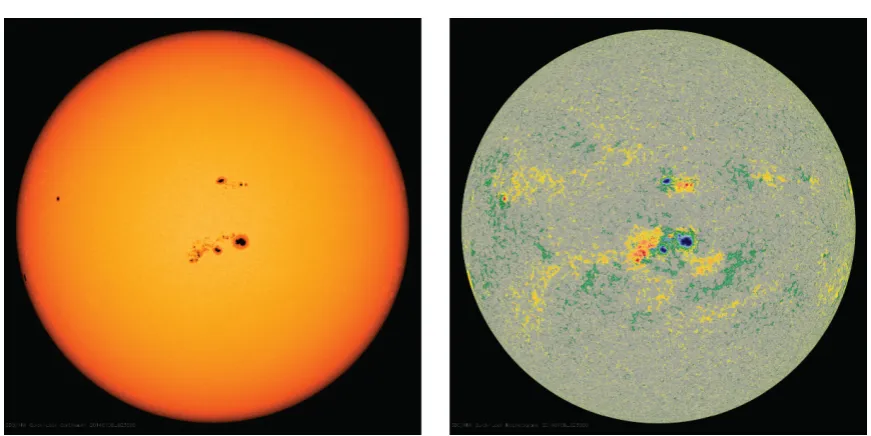
Figure 1.1:Continuum Image (left) and Magnetogram (right) of the Solar Disc taken with Nasa’s Solar Dynamics Observatory. These images were obtained in January 2014 when the Sun was in Solar maximum. The active region in the centre of the disc, AR 1944 was one of the largest Sun spot groups in the current cycle.
extrasolar planets.
This thesis will investigate a variety of asymmetries in exoplanet transit light curves caused by stellar activity in an attempt to reveal information about exoplanets and the host stars themselves.
1.1
Stellar Activity and Magnetic Fields
1.1.1
The Solar Cycle
The most extensively studied star is our own Sun. Observations of solar activity date back to the 17th-century, when Monks used pin-hole cameras to observe features on the Solar sur-face. Technology has since advanced, and satellites such as NASA’s Solar Dynamics Observat-ory (SDO) constantly monitor the Sun, providing a wealth of multi-wavelength photometry. Figure 1.1 shows a continuum image of the Sun taken with SDO (left image) and also the cor-responding magnetogram (right image). The continuum image clearly shows dark spots on the Solar surface. The magnetogram shows that the spots correspond to magnetically active regions on the Solar disc.
% 0 . 1 > % 1 . 0 > % 0 . 0 > -90 -45 0 45 90
1880 1890 1900 1910 1920 1930 1940 1950 1960 1970 1980 1990 2000 2010 Sunspot area in latitude strips (% of strip area)
Date (years)
La
titude (d
eg)
Figure 1.2: Solar butterfly pattern adapted from Hathaway (2010). The image shows the fractional coverage of the Solar disc by Sun spots as a function of time. The pattern is clearly cyclic, repeating over an eleven year period.
against time (Hathaway, 2010). The distribution of Sun spots clearly shows that the spots are restricted to two latitude bands on the surface of the Sun, one in each hemisphere.
At the start of each cycle, the spots appear at approximately±35◦. As the cycle progresses, the latitude of emergence moves towards the equator, culminating at a latitude of±5◦. The number of Sun spots on the surface of the Sun is not constant throughout the cycle, rather, the maximum number of spots appears when the latitude of emergence is around±15◦. This is known as Solar maximum and occurs midway through the cycle. Solar minimum occurs towards the end of the cycle and the start of the next cycle, at which point there may not be any spots on the surface of the Sun. Then, after eleven years, the pattern repeats. The shape of the Sun spot distribution has been called the “butterfly pattern”.
1.1.2
The Solar Magnetic Field
It was not until Hale (1908) took a spectrum of a Sun spot and compared it to a spectrum of the quiescent Sun that it was realised that Sun spots are magnetically active. The observations of Hale (1908) showed Zeeman splitting in the spectrum of a Sun spot that revealed the presence of a magnetic field of approximately 3kG in strength from the spot. Section 1.1.5 explains Zeeman splitting in more detail.
sun-Convective Zone
Radiative Zone
Omega Eff
ec
t
Alpha Eff
ec
t
Magnetic Buoyancy
Turbulence & Rotation
Magnetic Field Lines
[image:33.595.83.493.85.303.2]Magnetic Field Lines
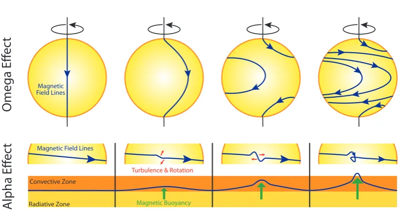
Figure 1.3: The two processes involved in the αΩ dynamo. The top panel shows how differential rotation causes the magnetic field lines to wind around the equator of the star. This process both stretches and strengthens the field lines. The bottom panel shows how magnetic buoyancy causes field lines to rise up through the convection zone. Turbulence then twists the field lines. This Figure is adapted with permission from William Ball, Imperial College.
rotation of the Sun) in a spot group to be of opposite polarity and that the corresponding spots in spot groups located in the other hemisphere of the Sun to also be of opposite sign (Hale, 1924). This can clearly be seen in the Solar magnetogram (right image in Figure 1.1). He also found that the polarity switched between Solar cycles. This lead to Hale believing that the magnetic field in the Sun was poloidal in geometry and originating deep within the Sun. Larmor (1919) put forward his theory that the magnetic field was induced by plasma motions within the Sun. He reasoned that because the Sun rotates differentially, the poloidal field will be sheared and will therefore produce field of opposite polarity in each hemisphere of the Sun. This process later became known as theΩeffect.
Contributions from Babcock (1961) and Leighton (1964) result in the current model for theαΩdynamo. Figure 1.3 shows a schematic of the process involved in theαΩdynamo. The current understanding of how the Sun’s magnetic field is generated requires the Sun to have a radiative core that is surrounded by a convective envelope. At the base of the convective envelope, in a thin interface layer known as the tachocline, dynamo processes produce the magnetic field. Extreme shearing of the field over the tachocline results in the field being amplified (Spiegel & Zahn, 1992).
1.1.3
Stellar Magnetic Fields
Unlike the Solar case, we are unable to resolve the discs of other stars to directly infer the presence of star spots and other tracers of magnetic activity; however, because stars rotate, their spectral signatures become broadened. This allows information about the geometry of features on the stellar surface to be recovered. This is known as Doppler Imaging. The spatial resolution of Doppler Imaging is determined by the rotation rate of the star and the timing between, and number of observations taken. The technique is particularly powerful for rapidly rotating, cool stars where the contrast between star spots and the quiescent photosphere is likely to be very large.
The first detection of a magnetic field on a star other than the Sun came from Babcock (1947). Babcock found Zeeman splitting in the spectrum of the star 78 Vir, which is inclined some 26◦ to our line-of-sight. From these observations, Babcock was able to determine that the star had a polar magnetic field strength of approximately 1.5kG.
A new approach for detecting magnetic fields on stars was first put forward by Semel (1989). Zeeman-Doppler Imaging (ZDI) was Semel’s solution to recovering the detailed struc-ture of the magnetic field on stars. ZDI is a tomographic imaging technique that allows the net large-scale magnetic field orientation and intensity to be reconstructed through a combination of Zeeman splitting and the Doppler effect.
1.1.4
The Zeeman Effect
No Magnetic
Field
Magnetic
Field
Spectra
Energy
Levels
1s
2p
Transitions
σ
π
σ
B
σ
σ
π
π
σ
σ
σ
σ
σ
σ
Figure 1.4: Simplified view of Zeeman splitting, adapted with permission from Reiners (2012). The left image shows how energy levels are split in the presence of a magnetic field. The right image shows the varous polarisation states of theπ,σblue, andσredcomponents.
associated total angular momentum quantum number (J= L+S) is able to split into (2J+1) states with magnetic quantum number M. The change between consecutive energy states is directly proportional to g B, where Bis the strength of the magnetic field, andg is the Landé factor. The Landé factor, which measures how sensitive the transitions are to the magnetic field, is a function of the spin and orbital angular momentum numbers and is given by:
gi =3
2+
Si(Si+1)−Li(Li+1)
2Ji(Ji+1)
. (1.1)
A transition between two energy levels must obey the rule that ∆Mi = −1, 0, 1. This rule results in there being three distinct types of transition, π component transitions obey
∆Mi=0, and theσredandσbluecomponents obey∆Mi =−1 and∆Mi= +1 respectively.
are linearly polarised and visible. Zeeman splitting is therefore subject to orientation effects. A convenient coordinate system for characterising the polarisation of the magnetic field are the Stokes parameters. The four components, Stokes I, Q, U, and V are defined as follows:
I = l + ↔, Q = l − ↔, U = -& − .%, V = − .
From these definitions, Stokes I measures the intensity of unpolarised light, but not the direction. Stokes Q and U measure the direction of linearly polarised light. Finally, Stokes V measures circular polarisation. The Stokes profiles are used throughout a variety of fields within observational astronomy because the polarisation of light can be measured with relat-ively straightforward instruments. Ideally for magnetic imaging, all four Stokes parameters would be measured; however, this is difficult to achieve observationally and so typically Stokes V is used as it has a larger signal-to-noise than Stokes Q and U.
1.1.5
Zeeman Doppler Imaging
Since the stellar disc is unresolved, reconstructing the magnetic topology is challenging due to flux cancellations in both linearly and circularly polarised light. As a star rotates, the angle between the vector components of the magnetic field and our line-of-sight changes. This therefore alters the Stokes components, enabling the magnetic field on the surface of the star to be reconstructed as a function of stellar phase. By using circularly polarised (Stokes V) spectral profiles coupled with a maximum entropy algorithm, Brown et al. (1991) were able to show that it is possible to reconstruct the magnetic configurations on Ap stars.
December 1996 December 1997
December 1998 December 1999
500
0
-500
Radial mag
netic field in
tensit
y (
[image:37.595.74.499.101.310.2]G)
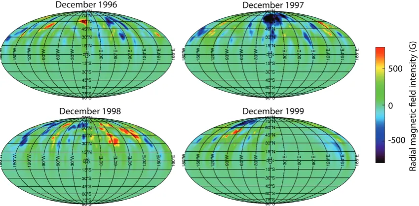
Figure 1.5: Reconstructed Zeeman Doppler Images of AB Doradus from December 1996, 1997, 1998, and 1999. The maps clearly show magnetic activity at all latitudes on the stellar surface (note the star is inclined to the observer and so the southern hemisphere of the star is not reconstructed). Images reproduced with permission from Donati & Collier Cameron (1997); Donati et al. (1999, 2003).
Whilst the method improves the signal-to-noise it does have some disadvantages. Princip-ally, the lines used to generate the mean profile are assumed to have similar profiles which means that any temperature dependence that could be present in the relative strengths of the signatures is lost.
A spectrum is then simulated assuming no magnetic field, B=0. This spectrum is then cross-correlated with the LSD spectrum and the χr2 statistic is computed. The assumed mag-netic field is then altered and a new simulated spectrum is produced and an updated value for theχr2statistic calculated. This process is iterated until the minimum value ofχ2r is obtained. The latest version of the ZDI code was developed by Donati et al. (2006). In this version of the code a spherical harmonic decomposition is invoked to reconstruct the magnetic topology on the stellar surface (see Appendix B). This has the distinct advantage of being able to place constraints on the allowed field geometry. The degree of complexity in the spherical harmonic reconstruction is set by limiting the allowed order of the fit,lmax. Morin et al. (2010) provide
a method for determining the largest value ofl,
lmax=max
2πv sini
FWHM ,lmin
, (1.2)
(1.2) represents the high v sinilimit where the line-broadening is due to the stellar rotation and the line profile can be seen as a one dimensional map of the photospheric magnetic field.
lmin is the assumed minimal resolution for a very low v sini and is typically taken to be 4 to
8. In this case the Doppler shift is small and the information on the magnetic field topology is recovered from the temporal evolution of the polarised Stokes signatures (Morin et al., 2010). Whilst ZDI is currently the most powerful technique for recovering the topology of stellar magnetic fields, it has some biases and limitations that are worthy of note. The technique firstly assumes the magnetic field to be static over the timescale of observation, i.e. all the acquired spectra are of the same magnetic field topology and strength. For rapidly rotating stars this is a valid approximation; however, it may be an issue for slowly rotating stars. Another limitation arises from the fact that two nearby regions of oppositely polarised light will cancel each other. The resolution of the recovered magnetic map is primarily limited by the rotation of the star. The rotational velocity of the star in our line-of-sight is given by v sini, the higher the value of v sini, the higher the resolution of the reconstructed magnetic map will be (Morin et al., 2008). Finally, the inclination of the star is important because if the star is edge on to our line-of-sight then the technique is unable to determine if a magnetic feature should be in the northern or southern hemisphere of the star.
Figure 1.5 shows Zeeman Doppler maps of the rapid rotator AB Doradus. The star has a rotational period of 0.5 days. Unlike Solar magnetograms, the magnetic maps of AB Doradus show the presence of very strong magnetic features at all latitudes of the star (the star is inclined to the observer meaning the southern hemisphere is unobservable) rather than being restricted to two active latitudes on the star.
1.1.6
Indicators of Stellar Activity
X-ray emission from the Sun was first detected by Blake et al. (1963). Since then, it has been shown that X-ray bright regions on the Solar disc originate from regions of closed magnetic field and X-ray dark regions correspond to regions of open magnetic field.
Figure 1.6: X-ray Images of the Solar disc from YOKOH taken over one Solar cycle (1991-2001). The images clearly show that during Solar maximum, the X-ray flux is larger than when the Sun is in minimum.
detected an X-ray luminosity of 1031erg s−1. Missions such as XMM-Newton, Chandra, and the ROSAT All-Sky Survey have lead to X-ray observations being detected on many more stars spanning the HR diagram. A clear correlation between stellar rotation rates and the level of X-ray emission was found by Vaiana & Rosner (1978) where they found higher X-ray emission values from rapidly rotating stars when compared to stars with slower rotation rates.
Another tracer for activity on stars comes from Ca II H and K emission. On the Sun, mag-netically active regions such as Sun spots emit Ca II H and K more intensely than magmag-netically inactive regions (Baliunas et al., 1995). The global emission of Ca II has been shown to dir-ectly correlate with the stellar magnetic field strength and coverage (Schrijver et al., 1989). The Mount Wilson Survey (Wilson, 1968, 1978) has monitored Ca II H and K emission on approximately one hundred main-sequence stars for many decades. The survey found that young stars have higher activity levels than older stars (such as the Sun). The survey also found that younger stars tend to be more rapidly-rotating. Stars with similar ages to the Sun were found to have lower activity levels and slower rotation rates (Baliunas et al., 1995).
1.1.7
Stellar Cycles
re-0.50 0.75 0.00 0.25 0.50 0.75 0.00 0.25 10 5 0 -5 -10 R adial M agnetic F ield (G)
June 2007 June 2008
[image:40.595.118.514.101.350.2]0.50 0.75 0.00 0.25 May 2009 0.50 0.75 0.00 0.25 June 2006 0.50 0.75 0.00 0.25 January 2010 0.50 0.75 0.00 0.25 January 2011
Figure 1.7:Zeeman Doppler Images showing the radial magnetic field of the planet hosting starτBootis obtained on June 2006, June 2007, June 2008, May 2009, January 2010, and January 2011. The star is shown in a polar projection down to a latitude of−30◦, with the Equator shown as a solid line. The tick marks represent the stellar phase where observations were taken. The maps clearly show the polarity of the pole reversing over time indicating the presence of a magnetic cycle. ZDI maps reproduced with permission from Catala et al. (2007); Donati et al. (2008); Fares et al. (2010).
2003). Along withτBootis, Morgenthaler et al. (2011) acquired ZDI maps of 19 Solar-type stars with masses ranging from 0.6−1.4M with rotation periods spanning 3.4−43 days obtaining ZDI maps between 2007 and 2011. They found that a number of these stars also exhibit magnetic cycles. The F star HD 78366, which is slightly larger than the Sun, and has a rotation period of approximately twice that of the Sun showed a three year magnetic cycle (Morgenthaler et al., 2011).
1.2
Exoplanets
The idea that planets could be found orbiting around stars other than the Sun is certainly not new. Struve (1952) correctly predicted that the presence of a Jupiter sized planet orbiting incredibly close to its parent star would cause a measurable shift in the stellar radial velocity. He also correctly predicted that should a planet orbit between us and its parent star, an eclipse would occur. By monitoring variations in star light over time one could indirectly detect the presence of a planet.
It was not until 1992 however, that the first extrasolar planet was discovered. Wolszczan & Frail (1992) reported the detection of a planet orbiting around the pulsar PSR1257+12. The first exoplanet discovered orbiting around a main sequence star was later found by Mayor & Queloz (1995). By observing the stellar radial velocity they were able to infer the presence of 51 Pegasi b. At the time, they reported the planet having a mass of 0.5−2MJ, orbiting at a
distance of 0.05 au from its host star (Mayor & Queloz, 1995). Since the initial discovery, the minimum mass of 51 Peg b has been refined toMpsini=0.45MJ(Marcy et al., 1997).
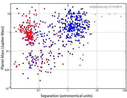
Since the discovery of 51 Pegasi b, the number of detected exoplanets has rapidly in-creased. There are now over one thousand known systems1. These systems have been dis-covered through a variety of different techniques. Figure 1.8 shows the currently known exoplanets. The Figure shows the distribution of orbital separation against planetary mass. The symbols are colour coded by detection method. Initially, the majority of exoplanets found by ground based transit and radial velocity surveys were typically Jupiter sized planets located fractions of an au to their host star. Due to their increased signal-to-noise, space based mis-sions such asKeplerare capable of finding smaller exoplanets located further away from their host star. The plot does not show theKeplercandidates which contain a number of Earth sized
0.1 1 10 100 10
1
0.1
0.01
10-3
Separation (astronomical units)
Planet Mass (
Jupiter Mass)
[image:42.595.101.530.88.419.2]exoplanets.org | 5/14/2014
Figure 1.8: The currently known exoplanets (May 2014). Plot obtained from
http://www.exoplanets.org. The red points correspond to planets found using the transit method. The blue points correspond to planets found through radial velocity observations. Microlensing discoveries are shown in green. Finally, directly imaged exoplanets are shown in orange. This Figure does not include the Kepler candidates published in Batalha et al. (2013) which include a number of Earth sized planets orbiting at distances beyond one au from their host star.
planets orbiting at distances of approximately one au Batalha et al. (2013). What follows is a brief description of the current techniques and missions for detecting and characterising exoplanets.
1.2.1
Radial Velocity
The presence of an exoplanet orbiting around a star moves the centre of mass of the system from the centre of the star. This means that the star now orbits around the common centre of mass of the system. As it does so, star light will be periodically blue and red shifted as the star moves towards, and away from the observer respectively. This process, known as the Doppler shift therefore provides an indirect method for inferring the presence of an exoplanet.
-0.2
0.0
0.2
0.4
0.6
0.8
1.0
1.2
-300
-200
-100
0
100
200
300
Phase
R
adial V
elo
cit
y
(m/s)
−100−0.04 0.00 0.04 [image:43.595.119.459.99.350.2]−50 0 50 100
Figure 1.9:Radial Velocity Curve of HD 189733. Reproduced with permission from Bouchy et al. (2005). The data has been phase-folded over the reported orbital period (2.2 days). The inset graph around zero phase clearly shows the Rossiter-McLaughlin effect that allows the spin-orbit alignment of the planet to be derived (see Section 1.2.3).
Bouchy et al. (2005)). The data is phase-folded over the orbital period of the planet (2.2 days). The best-fit Keplerian solution is displayed as a dashed line. The amplitude of the variation in the stellar radial velocity,K?, provides an estimate for the minimum mass of the exoplanet through the relation:
K?= 2πaMpsini
(Mp+M?)Pp1−e2
, (1.3)
where a is the semi-major axis of the planets orbit, MP is the mass of the planet, i is the orbital inclination angle, and e is the eccentricity. By assuming the stellar mass,M?, from the spectral type of the star a value for the minimum planetary mass, Mpsinican be derived. The radial velocity method has been the most successful method for finding exoplanets to-date. This is because a radial velocity signal can be detected for a wider range of orientations of the planetary orbit relative to the observer than the other methods.
0 2 4 6 8 1 0 Time (hours from 06:00 UTC on 05/09/2012)
0.997 0.998 0.999 1.000 1.001 1.002 1.003
[image:44.595.99.512.82.292.2]Normalised Flux
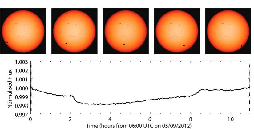
Figure 1.10:Transit of Venus, June 2012. Data from NASA’s SDO.
There have been many attempts at modeling the effects of star spots in radial velocity signals to try and remove them in order to reveal the presence of small exoplanets (see for example, Boisse et al. (2012)).
1.2.2
Transit Method
The transit method for detecting exoplanets requires monitoring the light received from stars and searching for periodic dips caused by the planet transiting over the stellar disc, blocking a fraction of the emitted star light. In our own Solar system, Venus and Mercury are occasionally known to transit between our viewpoint on Earth and the Sun. Such an event occurred on June 5th 2012 when Venus transited over the Solar disc. Figure 1.10 shows a continuum image sequence of the event with data from NASA’s SDO spacecraft. Shown below the image sequence is the light curve from SDO. The light curve clearly dips when Venus begins transiting and hence blocking Sun light.
The proportion of star light that a planet will block as it transits over the stellar disc is determined by the ratio of the area of the disc of the planet to the area of the stellar disc, i.e.
∆F=
R
p
R?
2
, (1.4)
based telescopes extremely challenging.
The transit method has some some advantages but also some disadvantages when com-pared to the radial velocity method. The main advantage is that the method only involves observing star light. This means that transit surveys can cover large numbers of stars at once. However, for a planet to be detected via a transit observation requires the orbit of the planet to be aligned such that the planet passes between our viewpoint on Earth and the host star. Horne (2003) calculated that the probability that a planet will transit decreases with orbital separation of the planet from it’s host star. This can be shown by considering that for a planet to be seen to transit, the disc of the planet must pass across the disc of the star, as seen from our perspective on Earth.
The impact parameter,
b=acosi, (1.5) defines the distance between the centre of the stellar disc and planet, wherei is the inclina-tion of the orbital plane of the planet relative to the observer. For the planet to transit, the inclination must be such thatacosi≤R?+RP. The direction of the normal to the orbital axis of the planet onto the sky is cosiand is uniformly distributed between 0−1. From this, the probability that a randomly inclined orbit satisfiesacosi≤R?+RP is given by
Pt =
R(R?+RP)/a
0 d cosi
R1
0 d cosi
=R?+RP
a ≈
R?
a . (1.6)
where Pt is the probability of transit.
Another issue with the transit method is that it is heavily biased towards finding exoplanets located close to their host star. Because the orbital period is related to the orbital separation through Kepler’s third law (P2∝ a3), a planet that is located closer to its host star will pass between our viewpoint on Earth and its host star more often than a planet that is located further away.
Ground based surveys such asSuperWASP2(Pollacco et al., 2006) are finding Jupiter sized planets located within 0.1 au of their host star. The SuperWASP consortium has currently detected over one hundred hot Jupiters. WASP-North in La Palma and WASP-South located in
South Africa are both comprised of two arrays of camera lenses attached to sensitive CCDs. They scan the night sky observing thousands of stars for transit events. Any suspected transit events are then followed up on larger telescopes.
Space based missions such asKepler3andCoRoT4are finding smaller exoplanets due to the enhanced signal-to-noise in the data they collect.Keplerwas scheduled to run for a minimum of 3.5 years, collecting continuous photometric data on over 150,000 stars in a single patch of sky. Due to mechanical failure, the satellite was only able to collect data for four years, but has still produced a number of confirmed planets and thousands of planetary candidates (Batalha et al., 2013). For these candidates to be confirmed, radial velocity follow up must be carried out. A new mission concept,K2will allow the Keplersatellite carry on observing specific regions of the sky for 83 days before having to rotate the spacecraft.
There are a number of pitfalls associated with the transit method. So-called “false-positives” are signatures in the stellar light curve caused by objects that are not planets creating a transit-like event. Small stars such as brown dwarfs are similar in size to Jupiter and so would create a transit signature in the light curve. However, such an object is much heavier than a Jupiter sized planet and therefore radial velocity measurements would reveal the object as a brown dwarf rather than a planet. For an object to be confirmed as a planet radial velocity ob-servations must be obtained to confirm the mass of the object. For transiting systems, the inclination of the star, i ≈ 90◦, and so sini ≈1 in Equation (1.3) meaning the mass of the object can be estimated to much greater accuracy than for non-transiting systems.
The depth of the transit provides the ratio of the planetary radius to stellar radius (Equa-tion (1.4)). If the host star was a giant star, such as an O star then a stellar companion would also provide a dip in flux of approximately 0.01. It is therefore important to look at the prop-erties of the host star as well and not solely the dip in flux caused by the transiting object alone.
The shape of the transit profile can also provide clues as to the type of object that caused it. Grazing binaries are other stars that do not entirely transit over the star of interest. Rather, they occult the limb of the stellar disc. Typically, these objects result in a V-shaped transit signature rather than the typical, flat bottomed U-shape of a planet transit.
Time (hours)
-2 -1 0 1 2
R adial V elo ci ty (ms
-1) 60
0
-60
Time (hours)
-2 -1 0 1 2
R adial V elo ci ty (ms
-1) 60
0
-60
Time (hours)
-2 -1 0 1 2
R adial V elo ci ty (ms
-1) 60
0
-60
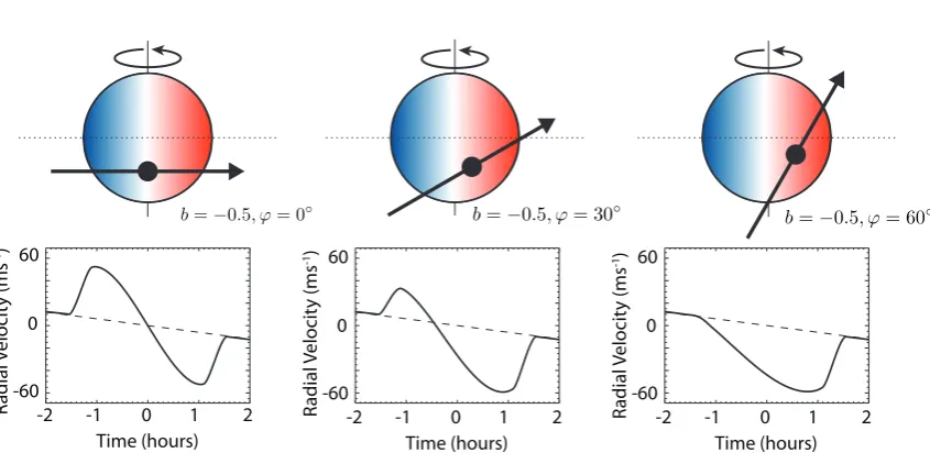
[image:47.595.78.501.82.288.2]b=−0.5, ϕ= 0◦
Figure 1.11: Illustration of the Rossiter-McLaughlin effect. Depending on the spin-orbit alignment between the stellar rotation axis and the orbital plane of the planet, the planet will occult different amounts of blue- and red-shifted light resulting in a different profile being recorded in the radial velocity curve. Adapted with permission from Gaudi & Winn (2007).
Systematics also hinder detecting exoplanets in stellar light curves. There are two types of noise present in the light curve. The first is purely Gaussian (white noise). The second is correlated noise, known as red noise (Pont et al., 2006). Red noise can be caused by astrophysical effects such as granulation on the surface of the star but also by systematics in the observations. For ground based surveys such as SuperWASP, sources of red noise can come from atmospheric effects such as transparency variations in the atmosphere or moon light. For both ground and space based missions, instrumental systematics, including hot pixels on the CCD and telescope instabilities can all result in red noise in the light curve.
1.2.3
Spin-Orbit Alignment of Transiting Exoplanets
Figure 1.12: Mircolensing light curve of OGLE-2005-BLG-390 reproduced with permission from Beaulieu et al. (2006).
Figure 1.11 shows how the spin-orbit alignment angle determines the resultant bump profile in the radial velocity curve for the same impact parameter, b=−0.5. In all cases, the transit light curve would look identical. In the first scenario, ϕ = 0◦, meaning the planet’s orbital plane is aligned with the stellar rotation axis. In this case, the planet will spend equal amounts of time blocking blue-shifted and red-shifted light and so a peak and subsequent dip of the same magnitude appears in the radial velocity profile. In the second example,
ϕ=30◦meaning that the planet spends less time blocking blue-shifted light and more time blocking red-shifted light. This results in a shorter peak and a longer dip in the radial velocity curve. Finally, in scenario 3, ϕ = 60◦ and the planet spends no time transiting over the blue-shifted part of the star. In this instance, only a dip is registered in the radial velocity profile. Therefore, combining radial velocity and transit observations allows us to determine the spin-orbit alignment of exoplanets.
1.2.4
Gravitational Microlensing
happens when the foreground star also hosts an exoplanet. The presence of a planet changes the gravitational field of the lens star, causing the magnification curve to deviate from the predicted model light curve. The timescale over which the planet alters the light curve is around a few days, much shorter than the whole microlensing event.
The event shown in Figure 1.12 shows one clear advantage of gravitational microlensing. The derived planetary mass of OGLE-2005-BLG-390Lb is 5.5 M⊕ with an orbital separation from its host star of a = 2.6 au. Gravitational microlensing is therefore able to find much smaller exoplanets that are located further from their host star when compared to the radial velocity and transit methods. The major downside to gravitational microlensing is that it requires the chance alignment of a foreground and background star, as such follow up obser-vations are not possible.
1.2.5
Direct Imaging
Directly imaging an exoplanet is incredibly difficult due to the brightness contrast between the host star and the planet. As with the radial velocity and transit methods for detecting exoplanets, direct imaging suffers from the bias that it is best suited to detecting very large, Jupiter sized planets orbiting nearby stars. One distinct difference between the direct imaging and the radial velocity and transit methods however, is that direct imaging works better for finding far-out planets where the planet can be separated in the image from the host star (Chauvin et al., 2004).
Figure 1.13 shows photometry of HR 8799 (Marois et al., 2010). The image clearly reveals the presence of four companion objects orbiting the star. Direct imaging allows the radius of the planet to be derived from the luminosity and temperature; however, the mass can only be derived from models.
1.2.6
Planetary and Exoplanetary Magnetic Fields
Figure 1.13: Detection of four exoplanets orbiting HR 8799 through direct imaging. Image reproduced with permission from Marois et al. (2010).
and Venus do not have a magnetic field; rather, the magnetosphere is caused by the Solar wind interacting with the upper atmosphere of the planet. The size of the magnetospheric cavity is principally determined by pressure balance between the planet’s magnetic field and the pressure from the Solar wind.
Figure 1.14 shows an illustration of the Solar wind interacting with Earth’s magneto-sphere. At the boundary between the Solar wind and Earth’s magnetosphere a bow shock forms. Typical Solar wind conditions result in this distance being approximately 10R⊕. For Jupiter, the Solar wind pressure is lower because the planet is located further from the Sun. The strength of the magnetic field is also considerably stronger than Earth’s magnetic field due to the different rotation rate and internal structure of the planet. This results in the mag-netosphere of Jupiter being much larger than Earth’s. Typically, the bow shock forms at a distance of approximately 50RJ from the surface of the planet.
Figure 1.14: Schematic showing the interaction between the Solar wind and Earth’s mag-netosphere. Image from SOHO, NASA.
Auroral Oval overlaid onto an image of the Earth.
Recently, this emission has been viewed from space by the Cluster mission (Mutel et al., 2008). It has been proposed that searching for radio emission could provide a method for detecting magnetic fields on exoplanets (Zarka, 2007). However, there have as yet been many unsuccessful attempts to detect radio emission from exoplanets (see for example, Bastian et al. (2000); Jardine & Cameron (2008); Smith et al. (2009)). There are a number of reasons that these attempts may have been unsuccessful, instrumental effects including a lack of sensitivity or geometric effects such as the beam of emission not being orientated so that we can observe it from Earth will all factor in our ability to detect radio emission from exoplanets.
1.3
Exoplanets and Stellar Activity
Both the radial velocity and transit method for detecting exoplanets involve monitoring vari-ations in light from stars. As such, stellar activity is a major hurdle when hunting for exoplan-ets using these methods. Dark star spots, and bright regions of plage on the stellar surface change the background light level from the star. Stellar activity therefore acts as a potentially significant source of red noise, the effect of which on active stars can be comparable to the signal from an exoplanet (Pont et al., 2006).
Figure 1.15: Southern auroral oval captured by NASA’s IMAGE satellite.
activity can reveal information about the host star itself. The four years of nearly continu-ous observations on approximately 150,000 stars provided byKeplermakes it an ideal stellar activity mission. Extended, continuous observations of stars will allow us to recover not only the rotation rate of the star, but potentially, differential rotation profiles as well. McQuillan et al. (2013) have carried out an auto-correlation analysis on the light curves of nearly 2000 main sequence planet-hosting candidates in theKeplercatalogue and found rotation periods for just over 700 of these stars. Interestingly, they find a lack of close-in planets orbiting around very rapidly rotating stars. A similar analysis has also been carried out by Walkowicz & Basri (2013) who also find a number of stars with rotation rates equal to their planet’s rotation period which provides tentative evidence for tidal interactions between these planets and their stars.