Case based reasoning in course timetabling: an attribute graph approach

Case-Based Reasoning Research and Development, Proceedings of the 4th International Conference on Case-Based Reasoning (ICCBR-2001). Vancouver, Jul-Aug, Canada, 2001. LNAI 2080. 90-104

Case-based Reasoning in Course Timetabling: An

Attribute Graph Approach

E. K. Burke1, B. MacCarthy2, S. Petrovic1, R. Qu1

1_{School of Computer Science and Information Technology, The University of Nottingham,} Nottingham, NG8 1BB, U.K

{ekb, sxp, rxq}@cs.nott.ac.uk

http://www.cs.nott.ac.uk/

2_{School of Mechanical, Materials, Manufacturing Engineering and Management,} The University of Nottingham, Nottingham, NG7 2RD, U.K

http://www.nottingham.ac.uk/school4m {[email protected]}

Abstract. An earlier Case-based Reasoning (CBR) approach developed by the

authors for educational course timetabling problems employed structured cases to represent the complex relationships between courses. The retrieval searches for structurally similar cases in the case base. In this paper, the approach is further developed to solve a wider range of problems. We also attempt to retrieve those cases that have common similar structures with some differences. Costs that are assigned to these differences have an input upon the similarity measure. A large number of experiments are performed consisting of different randomly produced timetabling problems and the results presented here strongly indicate that a CBR approach could provide a significant step forward in the development of automated systems to solve difficult timetabling problems. They show that using relatively little effort, we can retrieve these structurally similar cases to provide high quality timetables for new timetabling problems.

1.

Introduction

1.1 CBR in Scheduling and Timetabling Problems

It used CBR to solve the airlift management problem by decomposing the problem and then combining the retrieved cases for the new problem. Hennessy utilised the theory of scheduling in a CBR system presented in 1992 to solve the autoclave management and loading problem [2]. In 1993, Bezirgan developed CBR-1 for dynamic job shop scheduling utilising rules from a pool storing different methods [3]. Miyashita and Sycara implemented the CBR system called CABIN in 1994 [4]. This system addressed the job shop scheduling problem by retrieving previous repair tactics. MacCarthy and Jou proposed general CBR frameworks for scheduling in 1995 [5] and in 1996 they presented a survey about CBR research in scheduling [6]. In 1997, Cunningham proposed an approach to reuse portions of good schedules to solve traditional travelling salesman problems [7]. Schmidt, in 1998, stored scheduling tactics in the case base to help solving job shop scheduling problems [8].

Several types of timetabling problem are currently being studied such as course timetabling, exam timetabling, bus or rail timetabling and employee timetabling [9]. Our CBR system addresses educational course timetabling. The course timetabling problem was defined by Carter in [10]. It can be viewed as a multi-dimensional assignment problem. In a timetable, a number of courses are assigned into classrooms and a limited number of timeslots (periods of time) within a week. Students and teachers are assigned to courses.

Different timetabling problems have different constraints. This can make them very difficult to solve. A common constraint is ‘no person is assigned to two or more courses simultaneously’ which is known as a hard constraint because it should, under no circumstances, be violated. Other constraints known as soft constraints are desirable but it is not essential to satisfy them. Indeed, it would usually be impossible to satisfy all of them in a given problem. Examples are when two events should or should not be consecutive, or when one event should be before another.

In the early days of educational timetabling research, graph theoretic methods represented the state of the art [11]. Techniques like graph colouring were used to solve the problems. Other research using integer linear programming techniques to represent the timetabling problem was also carried out [12]. In more recent times, various meta-heuristic methods such as Tabu search [13], Simulated Annealing [14], Genetic Algorithms [15] and Memetic Algorithms [16, 17] have been employed to solve a variety of educational timetabling problems. Good results have been obtained in some specific problems by these approaches. A series of international conferences on the Practice and Theory of Automated Timetabling (PATAT) provides a forum for a wide variety of research work on timetabling and many relevant publications can be found in [18, 19, 20].

1.2 Structured Cases in CBR

The method of using a set of feature-value pairs to represent cases is heavily used in most traditional CBR applications [21]. The nearest-neighbour method has been used extensively and the similarity is obtained by calculating a weighted sum of the individual similarity between every feature-value pair of the case from the case base and a new case. However, in some domains, objects in the problems are heavily related, such as in the timetabling problem. The constraints between the events (exams, courses, meeting, etc) represent relations between objects in the problems. These relations affect their solutions significantly. A list of feature-value pairs is incapable of giving sufficiently important information about these relations to develop a solution. A similarity measure would be limited in reflecting the deeper similarities between the problems. Thus the retrieval process may not retrieve strongly similar cases in the case base without this important information. The adaptation based on these retrieved cases may be very difficult and may take as much effort as solving the new problem from scratch.

Structured cases have been discussed in the literature to represent problems with heavily inter-related objects, but no general theory or methodology has been identified. In most approaches, cases are represented by trees [23], graphs [24, 25] and semantic nets [24]. Many applications deal with the layout/design [26, 27] or planning problems [24, 25]. Gebhardt [28] provides more details of most existing CBR systems employing structured cases.

In [22] the authors presented an approach that employed attribute graphs to represent course timetabling problems structurally. The relations (constraints in the problems) between each pair of objects (courses in the problems) have a significant effect on the solution. The attribute graph represents a sophisticated level of knowledge about the constraints and the problem. The retrieval is also based on this information which is provided to find structurally similar cases for reuse. In this paper the proposed structured CBR approach for course timetabling problems is improved to deal with a wider range of problems than those dealt with in [22]. Section 2 describes the case base, the retrieval and adaptation processes of the proposed system. An analysis and discussions on a number of experiments carried out on the system is given in Section 3, followed by some concluding comments and directions for future work in Section 4.

2.

The Structured CBR Approach

2.1 Modelling Course Timetabling Problems by Attribute Graphs

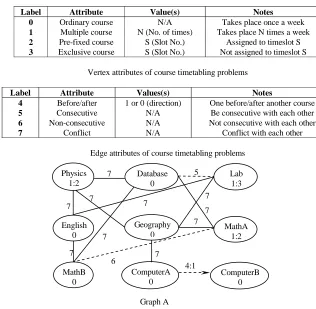
constraints and soft constraints are indicated by solid and dotted edges respectively. In the notation x:y, x is the label and y represents the value of the attribute. Physics, Lab and MathA are labelled by 1, indicating that they are multiple courses. Values 2, 3, 2 give the times they should be held per week respectively. Other courses labelled 0 (ordinary courses) should be held just once a week. The courses adjacent to edges labelled 7 cannot be held simultaneously. Database should be consecutive to Lab if possible (the edge between them is labelled 5) and MathA should not be consecutive to MathB if possible (the edge between them is labelled 6). The directed edge between

ComputerA and ComputerB is labelled 4, denoting that ComputerA should be held

before ComputerB.

Label Attribute Value(s) Notes

0 Ordinary course N/A Takes place once a week

1 Multiple course N (No. of times) Takes place N times a week

2 Pre-fixed course S (Slot No.) Assigned to timeslot S

3 Exclusive course S (Slot No.) Not assigned to timeslot S

Vertex attributes of course timetabling problems

Label Attribute Values(s) Notes

4 Before/after 1 or 0 (direction) One before/after another course

5 Consecutive N/A Be consecutive with each other

6 Non-consecutive N/A Not consecutive with each other

7 Conflict N/A Conflict with each other

Edge attributes of course timetabling problems

Fig. 1. A course timetabling problem represented by an attribute graph

2.2 The Graph Isomorphism Problem and the Retrieval Algorithm

The problem of finding structurally similar cases in the case base for a new case represented by attribute graphs is a graph or sub-graph isomorphism problem. This

7 7

6 7

7

7 7 7 5 7

7 7

MathA 1:2 Lab 1:3 Database

0

Geography 0 Physics

1:2

English 0

MathB 0

Graph A ComputerA

0

problem is known to be NP-Complete [29]. The approach we used in [22] was based on Messmer’s algorithm [30] in which all the possible (partial) permutations of the vertices representing (partial) graphs are stored in a decision tree. Those representing the same (sub-)structures are stored under the same node. In a decision tree, each node represents an attribute and has one child for each of the attribute’s values [31]. Our approach adapted this algorithm to build the case base into a decision tree that contains the attribute graphs of all the previous solved cases [22]. Each pair of attributes is assigned a value (individual similarities) to indicate how similar they are. If this individual similarity exceeds a given threshold, then it reports that these vertices or edges are not similar. The retrieval starts from the root node and classifies the new case into some nodes in the tree by comparing the permutations of the courses in the new case with those stored in the decision tree. Then all the (partial) permutations under these nodes have the same (sub-)structures with similar attributes of the new cases and will be retrieved to give a solution for the new problem. A similarity measure is given by a weighted sum of the individual similarities between the pairs of the matched vertices and edges. More details can be found in [22].

2.3 Retrieval of Structurally Similar Cases

Partially Similar Cases with Differences: The previous retrieval process [22]

retrieves the graphs of the cases from the case base that are graph or sub-graph isomorphic to the new case. However, cases in the case base that have common or partially similar (sub-)structures can also be reusable. In the retrieval phase developed here, not only the cases that are graph or sub-graph isomorphic to the new case are retrieved from the case base, but we also examine (partial) matches with some differences. We will describe this broader and more intelligent retrieval process in this section.

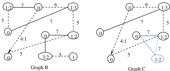
Cases in the case base need not contain all the corresponding similar edges in the new cases to be reused. For example in Fig. 2, graph B is neither graph nor sub-graph isomorphic to graph A shown in Fig. 1. However, graph B can be graph isomorphic to graph A if some vertices and edges are inserted. When dealing with difficult real world timetabling problems our approach has to be more flexible than just considering cases in the case base that are graph isomorphic to the new case. Note we can say that graph B is partially similar to graph A. In graph A, not all of its vertices and edges can match those of graph C in Fig. 2 (Physics, ComputerA and ComputerB cannot find a matching course in graph C). Also, not all of the vertices and edges in graph C can find a match with those in graph A (the course labelled with 1:2 with adjacent edges illustrated by light lines does not have a matching course with matching edges in graph A). These two cases have common parts that are partially similar with each other in either vertices or edges.

Fig. 2. Cases partially similar with some differences with case in Fig. 1

Similarity Measure: The similarity measure takes into account the costs assigned to

the substitutions, deletions and insertions of vertices and edges labelled with particular attributes from or into the new case. Deleting vertices and edges with different attributes from the cases in the case base are assigned lower costs than those of inserting vertices and edges into them. Also inserting and deleting the edges of hard constraints is assigned a higher cost than for the soft constraints. Costs are assigned so that the operations of deletion, insertion and substitution on the attribute graphs simulate the adaptation steps (explained in the later subsection) on the timetables retrieved. Deleting, inserting and substituting the less important vertices and edges has less of an effect on adapting the timetables. Thus such cases have lower costs assigned because of the need for less adaptation. The similarity measure between new case C2 and case C1 in the case base is presented in formula (1).

(1)

The notations in formula (1) represent the following: n: number of matched vertices

m, k: numbers of the vertices or edges needed to be inserted into and deleted from C2 respectively

pi,j: cost assigned for substituting vertex or edge i in C2 with vertex or edge j of C1 aa, dd: costs assigned for inserting and deleting a vertex or edge labelled with

attribute into and from C2

P: the sum of the costs of substitution of every possible pair of vertices or edges in C2 to those of C1

A, D: the sum of the costs of inserting and deleting all of the vertices or edges into and from C2 respectively

We can see that the closer the value S(C1, C2) is to 1, the more similar C1 and C2 are.

Branch and Bound in Retrieval: The retrieval needs to search through the decision

tree to find all the cases in the case base that are similar to the new case. The size of the decision tree storing all the possible permutations of the previous cases may be

D A P d a p C C S n j i m a k d d a j i + + + + −

=

∑

∑

∑

2 1, ) 1 ( 5 Graph B 5 4:1 7 5 6 7

5 ₇

1:2 1:3 1:2 0 0 0 0

3:2 1

large, resulting in extensive searching. Thus the retrieval process may be difficult and time consuming. Branch and bound [32] is employed to reduce the size of the search tree in the retrieval phase. When the permutation of the courses of the new case is input into the case base, the retrieval starts from the root node and first searches down along the branches as far as possible in the tree that stores the most similar (sub-)structures. All the possible candidate branches under one node that have a similar sub-structure and attributes with the new case are sorted by their summed costs. The branches storing the (sub-)structures whose costs exceed the given threshold are considered not to be similar to the (sub-)structures of the new cases and are all discarded. Thus the size of the search tree for retrieval can be greatly reduced because the retrieval does not need to search all the branches in the decision tree.

Backtracking is used when the retrieval cannot find a complete match. The retrieval backtracks to the parent node and the branch that has the lowest cost among the remaining branches will be chosen. This process continues until a complete match is found. All the complete and partial matches identified during the retrieval will be collected for potential adaptation.

Usually in timetabling problems, the more conflicts a course has with the other courses, the more difficult it is to schedule it. All the courses of the new case are sorted by their difficulties (here the degrees of the vertices in the attribute graph) in decreasing order and input into the decision tree for retrieval. Thus the retrieval process can first try to find the match for the more important courses.

Reuse and Adaptation of the Solutions: Adaptation of the timetables of all the

retrieved cases is performed according to the (partial) matches found. The adaptation steps for each retrieved case are:

1. According to the match found, matched courses are substituted and all the un-matched courses in the retrieved case are deleted.

2. All the courses that violate the constraints in the newly formed timetable are removed and inserted into an unscheduled list sorted by their difficulties in decreasing order. The courses in the new case that are not yet scheduled are also inserted into the sorted unscheduled list.

3. All the courses in the unscheduled list are rescheduled by the graph heuristic method described below.

Different constructive methods can be used to generate the timetables based on the partial solutions. The CBR approach presented here employs a simple graph heuristic method in the adaptation that is the same as that employed in [33] to construct a timetable based on the retrieved cases. It is briefly described below.

1. From the first one that is the most important, the courses in the unscheduled list are scheduled to the first timeslot with no violations (penalty-free);

2. The courses that cannot be assigned to a penalty-free timeslot will be scheduled to the timeslots that lead to the lowest penalty after all the others have been scheduled;

The best timetable with the lowest penalty is selected as the solution of the new case.

Penalty Function: Every timetable generated for the new case is evaluated by the

following formula (2):

Penalty = H X 100 + U X 100 + S X 5 (2)

Here H is the number of violations of hard constraints (the clashes between courses) and U is the number of unscheduled courses. H and U are assigned a cost of 100 to ensure that an infeasible timetable has a high cost. S is the total number of the violations of the soft constraints. They are assigned lower costs (at 5) because it is desirable to avoid them but not essential when a penalty-free timetable cannot be found. In different real-world timetabling problems, soft constraints could have different weights.

3.

Experiments with Different Case Bases and Course Timetabling

Problems

To test the computational performance of the system on different case bases, different groups of random cases with different features have been defined systematically and stored in the case base. The determination of a number of cases needed to build a case base is not an easy task. In order to have different case bases we generated cases with a range of properties that real-world problems may have. Thus an investigation of the system on a range of possible case bases can be carried out. Also different new cases are randomly generated so that the general performance of the system can be tested on a set of different new cases that the system may meet.

Fig. 3. Schematic diagram of the CBR system used for evaluation

3.1 Time and Memory Needed to Build the Decision Tree in the Case Base

In every case base we store 5, 10, 15 or 20 of the three types of cases. Table 1 gives the time spent and space needed to build these 12 different case bases. In the notation x/y, x gives the time in seconds and y is the number of nodes in the decision tree.

Table 1. Time spent on building the case base by 15-course simple, 15-course

complex and 20-course cases

5 10 15 20 15-simple

15-complex 20-simple

5.04/12689 8.48/23569 125.85/92449

12.58/32647 22.76/58475 273.84/141163

16.57/32647 46.88/93523 373.09/160887

24.83/52153 77.69/132750 598.36/193473

We can see that because the number of permutations grows explosively with the number of vertices in the graph, adding 20-course cases into the case base takes much more time and space than for both simple and complex 15-course cases. The time and number of nodes grows rapidly but not explosively with the number of cases in the case base. This is because many of the (partial) permutations of the cases may be stored under the node that is built for previous cases if they have the same (sub-)structures.

3.2 Time Spent in Retrieval

Table 2 gives the retrieval time for different new cases from the 12 different case bases. The values separated by ‘/’ give the retrieval time (in seconds) in the case base with 5, 10, 15 and 20 cases respectively. We can see that the retrieval time changes in the same way as that for building the same case bases.

15-simple cases 15-complex cases 20-simple cases

new case selection 5-course

new cases

15-course new cases 10-course new cases

5, 10, 15 or 20 cases

Case base

retrieval

adaptation by graph heuristic

method

Table 2. Retrieval time in different case bases

5-course new cases 10-course new cases 15-course new cases 15-simple 0.01/0.02/0.03/0.04 0.01/0.02/0.03/0.045 0.01/0.03/0.03/0.05 15-complex 0.01/0.03/0.2/0.2 0.02/0.04/0.5/0.3 0.02/0.2/0.6/0.3

20-simple 1.08/2.85/3.86/5.1 2.5/2.9/3.9/4.9 3.1/3.87/4.1/5.2

3.3 The Number of New Cases that Find Matches from the Case Base

With too few matched vertices, the retrieved cases cannot provide enough information for adaptation. Only matches that have enough courses (here more than half) in the retrieved cases are seen as helpful and retrieved for adaptation. From all the retrieved cases, a set of the most similar cases is selected as a set of candidates for the adaptation.

To test how many new cases can retrieve cases from the case base with different complexity, two groups of experiments were conducted on the case bases storing simple or complex 15-course cases. The results are given in Tables 5 and 6 respectively. The values before and after ‘/’ give the percentages of new cases that could retrieve partial and complete matches from the case base respectively. The values in parentheses give the overall percentage, as either partial or complete matches found.

Table 3. The percentages of new cases that find case(s) from the 15-course simple

case base No. of 15-simple cases in case base

5-course new case

10-course new cases

15-course new case

Average percentages

5 100/100 (100) 100/0 (100) 30/0 (30) 76.67

10 100/100 (100) 100/0 (100) 70/0 (70) 90

15 100/100 (100) 100/0 (100) 70/0 (70) 90

20 100/100 (100) 100/45 (100) 70/0 (70) 90

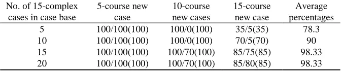
Table 4. The percentages of new cases that find cases from the 15-course complex

case base

No. of 15-complex cases in case base

5-course new case

10-course new cases

15-course new case

Average percentages

5 100/100(100) 100/0(100) 35/5(35) 78.3

10 100/100(100) 100/0(100) 70/5(70) 90

15 100/100(100) 100/70(100) 85/75(85) 98.33

It can be seen from Table 3 that all of the 5-course and 10-course new cases can find (partial) match(s) from a case base with simple 15-course cases. No complete match can be found for new cases with 10 or more courses when the case base consists of less than 20 cases. Table 4 shows that storing complex cases in the case base enables more new cases to find matches. Higher percentages of larger new cases (10-course and 15-course new cases) retrieve cases (complete or partial matches) from the case base.

We can also see that when 10, 15 or 20 simple cases are stored in the case base, the same number of new cases (90%) can retrieve matches. Also, the same number of new cases (98.3%) can find matched cases in the case bases with 15 or 20 complex cases. This is because the attribute graphs of a certain number of cases in the case base provide a certain number of different (sub-)structures in the decision tree. Additional cases do not provide new (sub-)structures in the decision tree. Attribute graphs of complex cases can provide more (sub-)structures, thus more new cases can retrieve cases from the case base with more than 10 or 15-course complex cases.

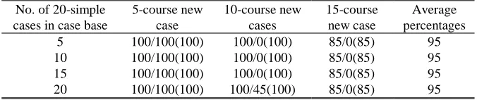
The effect of storing larger cases with 20 courses in the case base is tested in a further experiment and the results are given in Table 5. The overall percentages of successful retrievals are higher than those with smaller simple cases but lower than those with smaller complex cases.

Table 5. The percentages of new cases that find cases from the 20-course case base

No. of 20-simple cases in case base

5-course new case

10-course new cases

15-course new case

Average percentages

5 100/100(100) 100/0(100) 85/0(85) 95

10 100/100(100) 100/0(100) 85/0(85) 95

15 100/100(100) 100/0(100) 85/0(85) 95

20 100/100(100) 100/45(100) 85/0(85) 95

0 20 40 60 80 100 120

1 3 5 7 9 11 13 15 17 19

No. of cases in case base

Perc

ent

ages

of

new

c

a

s

e

s

t

hat

f

ind

m

a

tc

hed c

a

s

e

(s

)

15-simple

15-complex

20-simple

Fig. 4. Percentage of new cases that retrieve case(s) from different case bases

3.4 Adaptation of Retrieved Cases

20 different cases with 5, 10 or 15 courses are tested on the case bases with 5, 10 15 or 20 of the three types of cases respectively. So altogether 720 (=20×3×4×3) experiments were carried out. The graph heuristic method described in Section 3 is used in the adaptation to adapt all the retrieved cases and the timetable that has the lowest penalty is used as the solution for the new cases. For comparison, the same graph heuristic method is also used to generate a timetable from scratch for each new case that can retrieve cases from the case base. All the timetables generated by these methods are evaluated by using the penalty function given in (2). The number of schedule steps needed during adaptation is also taken into account in the comparison. The average penalties and schedule steps for these two methods are presented in Tables 8, 9 and 10. The y in ‘x/y’ gives the number of schedule steps needed to obtain a timetable that has a penalty x. Values in parentheses give the penalty and schedule steps of the timetables generated by adapting complete matches for the new cases.

Table 6. Penalties and schedule steps by graph heuristic (GH) and CBR approach

with different 15-course simple case bases

5-course new case 10-course new cases 15-course new case No. of

cases _{CBR GH CBR GH CBR GH}

5 6/7(6/8) 11/15 22.8/35.8 30.5/45.6 39.2/68 39.2/76

10 6/6(5/6) 11/15 16.5/30.2 30.5/45.6 33.2/59 36.1/59

15 6/6(5/6) 11/15 16.5/30.3 30.5/45.6 33/59.8 36.1/69

Table 7. Penalties and schedule steps by graph heuristic (GH) and CBR approach

with different 15-course complex case bases

5-course new case 10-course new cases 15-course new case No. of

cases _{CBR GH CBR GH CBR GH}

5 7/7(6/5) 11/15 19.3/30.5 30.5/45.6 30/49 15/50

10 6/6(6/5) 11/15 18.5/31.2 30.5/45.6 30/49 15/50

15 6/6(5/5) 11/15 17/31(28/39) 30.5/45.6 30/60(39/65) 39.7/69 20 6/6(5/5) 11/15 16/27(28/39) 30.5/45.6 27/61(39/68) 39.7/69

Table 8. Penalties and schedule steps by graph heuristic (GH) and CBR approach

with different 20-course case bases

5-course new case 10-course new cases 15-course new case No. of

cases _{CBR GH CBR GH CBR GH}

5 6/6.7(5/6) 11/15 16.5/28.7 30.5/45.6 37.9/55 40/66.4 10 6/6(5/5.5) 11/15 15.8/28.3 30.5/45.6 36.8/55.7 39.4/67 15 6/6.5(5/5.3) 11/15 16.4/27.3 30.5/45.6 61.7/79.3 53.4/81 20 6/6(5.3/5.4) 11/15 18/29(10/4) 30.5/45.6 62.2/76.5 46/72.4

From the results shown in Tables 8, 9 and 10 we can see that in all of the experiments solving 5-course and 10-course new cases, the timetables constructed by the graph heuristic method based on the partial solutions from the proposed CBR approach need much fewer scheduling steps and have less penalties than those constructed from scratch using the graph heuristic (GH) approach. The knowledge and experiences stored in the previously solved problems that are structurally similar to the new problems are re-used and not too much effort needs to be taken to get high quality results.

In solving the larger 15-course new cases by the case base with 5 or 10 15-course complex cases, the CBR approach finds timetables with higher penalties than those from the graph heuristic approach and takes almost the same number of schedule steps in adaptation. This is because only storing a small number of (less than 10) complex cases cannot provide enough good cases (sub-structures) and the complexity of the retrieved cases makes the adaptation difficult. Storing more complex cases provides much better results. Also, larger retrieved cases may cause more adaptation because more courses in the timetables of these cases may need more adaptation. This is why in Table 8 some of the retrieved larger cases provide high penalty timetables for the new cases.

4

Conclusions and Future Work

The CBR approach described in this paper avoids large amounts of computation and provides good results in solving timetabling problems. It shows that the retrieved cases that have similar (sub-)structures can provide high quality partial solutions for the new cases. This is because by retrieving structurally similar cases from the case base, solutions generated on similar constraints may be easily reused for the new case without significant adaptations. Timetables constructed by using the graph heuristic method on the basis of these partial solutions take less scheduling effort to get lower penalty solutions than those constructed by only using the same graph heuristic method from scratch.

The CBR system also shows that storing a certain number of cases in the case base can provide the same number of (sub-)structures as those obtained by storing more cases. We found that storing a certain number of complex cases works better than storing larger or more simple cases for providing the sub-structures for re-use. It is the number of (sub-)structures, not the number of cases in the case base that contributes to the successful retrieval of partial solutions for adaptation. It is important to build a case base with just a certain number of cases because the size of the decision tree grows rapidly when the size and the number of the cases in the case base increases.

The current approach gives promising results on solving relatively small problems. This provides a good basis for solving larger problems. Research is now being undertaken for solving larger timetabling problems based on the current system. All the cases in the current system are produced randomly to test the general performance. Tests on real-world specific timetabling problems will also be carried out. Other adaptation methods will also be studied in future work.

It is also likely that this CBR approach in timetabling can be used to solve more general problems in other domains that have inter-related objects and that can be modelled using attribute graphs.

References

1. Koton P.: SMARTlan: A Case-Based Resource Allocation and Scheduling System. In: Proceedings: Workshop on Case-based Reasoning (DARPA). (1989) 285-289

2. Hennessy D., Hinkle D.: Applying Case-Based Reasoning to Autoclave Loading. IEEE Expert. (1992) 7: 21-26

3. Bezirgan A.: A Case-Based Approach to Scheduling Constraints. In: Dorn J., Froeschl K.A. (eds): Scheduling of Production Processes. Ellis Horwood Limited. (1993) 48-60

4. Miyashita K., Sycara K.: Adaptive Case-Based Control of Scheduling Revision. In: Zweben M., Fox M.S. (eds): Intelligent Scheduling. Morgan Kaufmann. (1994) 291-308

5. MacCarthy B., Jou P.: Case-Based Reasoning in Scheduling. In: Khan M.K., Wright C.S. (eds.): Proceedings of the Symposium on Advanced Manufacturing Processes, Systems and Techniques (AMPST96). MEP Publications Ltd. (1996) 211-218

7. Cunningham P., Smyth B.: Case-Based Reasoning in Scheduling: Reusing Solution Components. The International Journal of Production Research. (1997) 35: 2947-2961 8. Schmidt G.: Case-Based Reasoning for Production Scheduling. International Journal of

Production Economics. (1998) 56-57: 537-546

9. Wren V.: Scheduling, Timetabling and Rostering – A Special Relationship? In: Burke E.K., Ross P. (eds.): The Practice and Theory of Automated Timetabling I. Lecture Notes in Computer Science 1153. Springer-Verlag: Berlin (1996) 46-75

10.Carter M.W., Laporte G.: Recent Developments in Practical Course Timetabling. Burke E.K., Carter M. (eds.): The Practice and Theory of Automated Timetabling II. Lecture Notes in Computer Science 1408. Springer-Verlag: Berlin (1998) 3-19

11.Werra D.: Graphs, Hypergraphs and Timetabling. Methods of Operations Research (Germany F.R.). (1985) 49: 201–213

12.Tripathy A.: School Timetabling - A Case in Large Binary Integer Linear Programming. Management Science. (1984) 30:1473–1489

13.Dowsland K.A.: Off-the-Peg or Made to Measure? Timetabling and Scheduling with SA and TS. In: The Practice and Theory of Automated Timetabling: Selected Papers from the 2nd International Conference. Springer-Verlag: Berlin. (Lecture Notes in Computer Science 1408). (1998) 37-52

14.Thomson J.M., Dowsland K.A.: General Cooling Schedules for a Simulate Annealing Based Timetabling System. In: Burke E.K., Ross P. (eds.): The Practice and Theory of Automated Timetabling I. Lecture Notes in Computer Science 1153. Springer-Verlag: Berlin (1996) 345-364

15.Erben W., Keppler J.: A Genetic Algorithm Solving a Weekly Course-Timeatbling Problem. In: Burke E.K., Ross P. (eds.): The Practice and Theory of Automated Timetabling I. Lecture Notes in Computer Science 1153. Springer-Verlag: Berlin (1996) 198-211

16.Burke E.K., Newell J.P., Weare R.F.: A Memetic Algorithm for University Exam Timetabling. In: Burke E.K., Ross P. (eds.): The Practice and Theory of Automated Timetabling I. Lecture Notes in Computer Science 1153. Springer-Verlag: Berlin (1996) 241-250

17.Paechter B., Cumming A., Norman M.G., Luchian H.: Extensions to a Memetic Timetabing System. In: Burke E.K., Ross P. (eds.): The Practice and Theory of Automated Timetabling I. Lecture Notes in Computer Science 1153. Springer-Verlag: Berlin (1996) 251-265

18.Burke E.K., Ross P.: The Practice and Theory of Automated Timetabling: Selected Papers from the 1st International Conference. Springer-Verlag: Berlin. (Lecture Notes in Computer Science 1153). (1996)

19.Burke E.K., Carter M.: The Practice and Theory of Automated Timetabling: Selected Papers from the 2nd International Conference. Springer-Verlag: Berlin. (Lecture Notes in Computer Science 1408). (1998)

20.Burke E.K., Wilhelm E.: Proceedings of the 3rd _{International Conference on Practice and} Theory of Automated Timetabling. To be published by Springer-Verlag: Berlin. (2001) 21.Watson I., Marir F.: Case-Based Reasoning: a Review. The Knowledge Engineering Review.

(1994) 9: 327-354

22.Burke E.K., MacCarthy B., Petrovic S., Qu R.: Structured Cases in CBR – Re-using and Adapting Cases for Timetabling Problems. Journal of Knowledge-based System. (2000)

13(2-3): 159-165

23.Ricci F., Senter L.: Structured Cases, Trees and Efficient Retrieval. Proceedings of the Fourth European Workshop on Case-based Reasoning. Springer-Verlag: Dublin. (1998) 88-99 24.Sanders K.E., Kettler B.P., Hendler J.A.: The Case for Graph-Structured Representations.

25.Andersen W.A., Evett M.P., Kettler B., Hendler J.: Massively Parallel Support for Case-Based Planning. IEEE Expert. (1994) 7: 8-14

26.Börner K.: Structural Similarity as Guidance in Case-Based Design. In: Wess S., Althoff K.D., Richter M. (eds): Topics in Case-based Reasoning. Springer-Verlag: Kaiserslautern. (1993) 197-208

27.Börner K., Coulon C.H., Pippig E., Tammer E.C.: Structural Similarity and Adaptation. In: Smith I., Faltings B. (eds): Advances in Case-based Reasoning. Springer-Verlag: Switzerland. (1996) 58-75

28.Gebhardt F.: Methods and Systems for Case Retrieval Exploiting the Case Structure, FABEL-Report 39, GMD, Sankt Augustin. (1995)

29.Garey M.R., Johnson D.S.: Computers and Intractability: A Guide to the Theory of NP-Completeness. Freeman and Company: New York. (1979)

30.Messmer B.T.: Efficient Graph Matching Algorithms for Preprocessed Model Graph. PhD thesis, University of Bern. (1995)

31.Quinlan J.R.: Induction of Decision Trees. Machine Learning. Morgan Kaufmann (1986) 1: 81-106

32.Williams H.P.: Model Building in Mathematical Programming. Wiley: Chichester. (1999) 33.Burke E.K., Elliman D.G., Weare R.F.: A University Timetabling System Based on Graph