doi:10.4236/cn.2010.21004 Published Online February 2010 (http://www.scirp.org/journal/cn)
Neural Network Performance for Complex
Minimization Problem
Tadeusz Wibig
Physics Department, University of Lodz; Cosmic Ray Laboratory, The A. Soltan Institute for Nuclear Studies, Uniwersytecka 5, 90-950 Lodz, Poland
E-mail: [email protected]
Received October 19, 2009; accepted November 11, 2009
Abstract: We have analyzed the important problem of contemporary high-energy physics concerning the es-timation of some parameters of the observed complex phenomenon. The standard statistical method of the data analysis and minimization was confronted with the Neural Network approaches. For the Natural Neural Networks we have used brains of high school students involved in our Roland Maze Project. The excitement of active participation in real scientific work produced their astonishing performance what is described in the present work. Some preliminary results are given and discussed.
Keywords: artificial neural network, natural neural network, curve fitting, minimization, interpolation, optimization
1. Introduction
The analysis of the surrounding physical reality, for last at least three thousand years, as we know it, follow the line of building simplified models and solving problems using specific tools developed with applied approximations making them easy or relatively easy to maintain. The unquestioned successes of such, scientific, way of think-ing allow us to create so-called civilization.
However, this method can have limitations. Some problems can not be treated this way, at least at present. There is a belief that, e.g., mathematical tools needed to solve some problems in quantum field theory or hydro or thermodynamic will be developed in the future. How-ever there are much common problems where the usual methods of standard analysis sometimes fail. The gen-eral problem of ‘pattern’ recognition is the perfect ex-ample.
We would like to discuss here a particular problem of the describing of the data registered by some cosmic ray physics experimental device. This is a problem of the general class of minimization or curve fitting. It is a good example to illustrate our general statement.
The statement is that the complex problems can be solved not only qualitatively but also quantitatively on the level of the standard statistical method precision not only by Artificial Neural Network (ANN) trained on the problem but with the over-sized, redundant Natural Neu-ral Network (NNN) using their ‘natuNeu-ral’ abilities gathered in the past not obviously (obviously not) related to the particular problem.
The method of the analyzing the NNN performance is described and some first results are given in this paper.
2. The Problem
The ultra high-energy cosmic ray particles, its origin and nature are one of the most intriguing questions on general interest among the physicists. The phenomenon of arriv-ing form the cosmos of the elementary particle with en-ergy of about 50 J is very rare and thus hard to investigate experimentally. Fortunately during the passage through the earth atmosphere the cascade of smaller energy sec-ondary particles is created and eventually the surface is momentarily bombarded by billions of particles spread over the area of squared kilometers. The experimental setups for registrations of such events consists of several to several thousands detectors separated by hundreds of meters to few kilometers equipped with the triggering and recording devices.
T. WIBIG 32
only to get the precise enough estimates of normalization constant total number of particles, first or at last second moment of the distribution (or any other, more suitable, parameters of this distribution). For doing this one has to use some prior assumptions, e.g. about the radial sym-metry or the expected analytically approximated func-tional form of the distribution. After that one has to go through the procedure of making the estimate.
The standard is to make a χ2 or likelihood measure of
the goodness of the fit and than to use known textbook methods to minimize the respective distance between the ‘theoretical line’ and ‘measured points’.
In general this is all we need, but practically there are classes of multiparameter problems and very noisy data when the minimization is not very straightforward. This is of course also the problem of the function to be minimized and its many local minima, distant and not very much different in depth. The problem of Extensive Air Shower (EAS) parameter estimation is a good example. The number of parameters is not very large. From physical point of view they are mainly: position of the shower axis and total number of particles and a parameter of the slope of theirs radial distribution. For simplicity and using the prior knowledge on the shower physics we use only one shape parameter [1]. The large spacing between detectors makes this simplification justified. We neglect also, for the purposes of this paper, the two parameters describing shower inclination. So we have only four parameter space with well defined physical meaning. It also provides a kind of independence of them all which is very helpful for minimization.
The problem arises because of the sharpness of the dis-tribution of particles when one tests the distances close to the shower axis. When the detector gets close to the axis number of registered particles goes into thousands while a little far it goes to tens being on the edge of 1 and below in most other detection points. From the point of view of minimization procedure when the axis position is tested close to the one detection point it is the only one which controls the χ2 or likelihood or whatsoever. This situation
is caused by the physics of the process and one can’t avoid it. The exclusion of close detectors is a remedy, but it is rather costly. The detector close to the shower core reg-istered highest number of particles and thus the statistical importance of this point is the highest and in case of small number of detection points in general we can’t afford to lose the most important one. We have to play with it.
Many methods and tricks were invented to get the minimization going with a number of problems as less as possible, but, as it will be shown, it is a hard task. The parameter which we will study comparing different methods of estimation is the number of lost events. We can define here the lost events as that having the χ2 (or
other studied measure) above some critical value. But to be comparable with others we defined them as the events
for which the minimization moves the values of the pa-rameter of the axis position: x and y and shower size
ex-ceeding some limits (which can be treated as defining the divergence of the minimization procedure).
3. Artificial Neural Network Approach
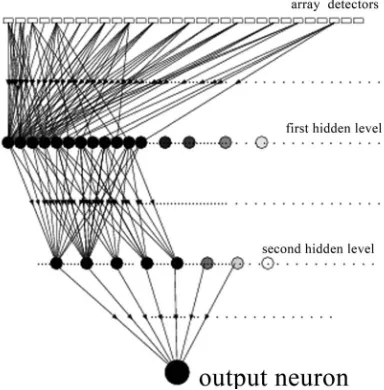
The process of estimation EAS parameters with the help of Artificial Neural Network, as it is shown in [5] in the case of the hard shower component registered by the experiment KASCADE [4], can be quite successful. In the present work we used very similar network architec-ture which schematic view is shown in Figure 1. The input nodes are seeded with the registered particle densi-ties, and the signal processing eventually gives the total number (its logarithm, to be precise) of shower particles. The particular network was build to work with the array of the Roland Maze Project being realized in Lodz [2]. The array is based on detectors placed on the roofs of city high school. In the final phase about 30 schools will be equipped with 4 one squared meter scintillator detec-tor each. The sum of numbers of particles registered in each school carry the same information as the four num-bers from all four detectors due to the Poissonian char-acter of the cascade. The distance of about 10 meters within each school are negligible with the kilometers between the schools and the scale of the changes of the average particle density. Thus we need the ANN with 30 input nodes. The geometry of the network we used here was not optimized for the number of neurons and its final structure analyzed here is highly redundant. We used eventually two hidden layers with 20 and 10 neurons, respectively.During tests we check that the input values could be logarithms of the value of the input signal surface enlarged by 1.0 to avoid the zeros from detectors with no muon registered. We do not add the electronic noise here as not very big. Each input is connected with each of the first hidden level neurons. The last hidden level neurons are connected to the single output unit. Tests with differ-ent number of hidden neurons shows that there is no ef-fect on the network performance when we keep this numbers with reasonable limits. The number of the net-work parameters to be trained was from about 5000 to 25000. As the neuron response function the common sigmoid has been used. The network was trained with the standard back-propagation algorithm using the simple ‘EAS generator’.
ac-cording to the flat distribution in logarithm of particle energy scale. The cosmic ray shower spectrum is known to be of the power-law form and it is very steep with the index of about -3.0. This affects the estimated values. The generation used allows for the systematic bias, but on the other hand, too steep distribution in the training sample leads to the over-training of network with small size events while the events of energies, e.g., 100 times bigger, which are million times less abundant are practi-cally not used for the training purposes. The uniform in log(E) is the compromise prior.
The steep spectrum makes the registered events consist mostly of events on the lower primary particle energy threshold which is defined by the trigger requirements. The ‘artificial trigger’ was applied to the training sample. We assumed that at least three ‘schools’ has to register some particles at least in two detectors each. Such trigger can be realized in the original Roland Maze Project array.
With the information limited so much, it is expected that standard minimization should fail quite often. The comparison of effectiveness of the standard and the ANN approach is one of the questions we want to answer here.
The network was trained first to estimate the most important shower parameter: the shower size (the total number of particles in the shower at the observation level). But we tested also the possibility of using network to estimate other parameters, and it was found that there is possible to train the network to estimate as well the x- and y-coordinate of the shower axis. The attempt to get the age
parameter was not very successful.
In the Figure 2 the convergence of the training proce-dure is shown for the network trained with shower size a) and the axis position b). The dependence of the width of the distribution of the deviation of the estimated value from the true one is shown. The learning is quite a long
lasting process. The first rational answers appear how-ever already after the number of training events compa-rable with the number of internal weights. Then we ob-serve the continuous improvement. An interesting feature appeared below 1 million events on Figure 2b. There are abrupt decreases of efficiency and then further and deeper improvements. The effect is seen for all networks we tested for both x- and y- axis position adjustment. It is
seen always at the roughly some point and we suggests that it means the internal change of the network strategy of estimation. Something similar is seen also for EAS size estimation networks but at different length of train-ing sample (around 104 at Figure 2a). The closer look at
this phenomenon could put some light to the process of network learning but it is beyond of the scope of this paper.
We ended the learning process at the 108 event sample.
[image:3.595.313.505.83.278.2]The further improvement is interesting, but of no practical importance. The final state of the trained network allows us to use it as a tool for shower size and axis position determination. Such trained network was then applied
Figure 1. Schematic layout of the Artificial Neural Network used for the evaluation of the total number of the EAS par-ticles
to the serial of 10000 events produced by the particles of energy generated by our event generator which build the library of the showers to by analyzed also with different methods. The ANN, when any event from the library is taken as an input, always give some answer. The accuracy of the ANN answer was studied in few ‘modes’.
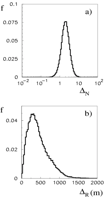
In the Figure 3 the illustration of an accuracy is pre-sented as histograms showing the spread of the ANN guess errors. To get it easier to compare with other method some numbers should be given. Some measures of the ‘goodness of the fit’ are given below.
σN - the accuracy of size determination measured as a dispersion of the difference between decimal logarithms of the true and ANN reconstructed shower size (total
number of particles).
ΔN - the bias of the shower size measured as a differ-ence of the average true and ANN reconstructed shower
size.
ξN - the fraction of perfect reconstructions, which we
defined as these within 10% around the true value of the
shower size (logarithm).
σR - the error in the localization measured as a average distance between true and ANN reconstructed shower
axis position.
ξR - the fraction of perfect localizations, by which we
mean the ANN reconstructed axis closer than 100 m from
the true one.
The values of all these five parameters obtained for our trained network are given in the Table 1 in the sec-ond column, labeled ANN.
4. Standard Minimization Approach
T. WIBIG 34
Figure 2. The accuracy of the ANN answer as a function of the number of events using for the training process shown as a widths of the distribution of the difference between the decimal logarithm of the estimated shower size and the ‘true’ value a), and the difference of the respective spatial distance (in one x direction) difference b). Different lines represents different shower size samples. The solid one is for showers of the “true” size between 3 and 5109 particles (the medium sizes), the dashed is for smaller showers, and the dotted one for really big showers
were also analyzed with the help of standard numerical minimization algorithms. We have used the CERN MIN- UIT package described in [3]. The straightforward ap-plication for such, not perfectly well determined, problem as shower parameter minimization works rather bad, so some slightly improved, thus much time consuming pro-grams reaching the minimum of the likelihood in few steps, have to be developed. After careful adjustments of the proper divergence between ‘the data’ and predictions the program runs better. We have to mention here that some oversimplification was made here, because the radial distribution of shower particles used for minimiza-tion was exactly the one which was used inside the gen-erator to calculate the averages. In the real case the parti-cle distribution is rather unknown. This fact favours the minimization technique and the results given in this work should be treated with care, as the optimistic limit. After applying to the library showers, the same as
ana-lyzed with the help of ANN, the results are as they are shown in the Table 1 in the columns labeled ‘MINUIT’. There are two values in each case. The first on gives the average over all studied showers (we limited parameter ranges to reasonable values). Some showers due to the fluctuations can not give the minimum within the as-sumed ranges of parameters of the minimum found gives the value of χ2 too high to be accepted. If we excluded
[image:4.595.340.509.195.515.2]them from the averaging procedures, the results get better
Figure 3. The spread of the trained ANN answer for the shower size a) and the spatial distance b) between guess and the true size and position of the shower axis. The result is obtained for the library showers
Table 1. Comparison of the performance of ANN, standard minimization and the three best NNNs found in our ex-periment
ANN MINUIT NNN
σN 0.217 0.478 0.280 0.270 0.279 0.294 0.349
ΔN 0.29 -0.14 0.14 0.31 0.97 1.29 0.01
ξN 6% 17% 20% 16% 17% 12% 13%
σR 442 567 312 375 613 528 662
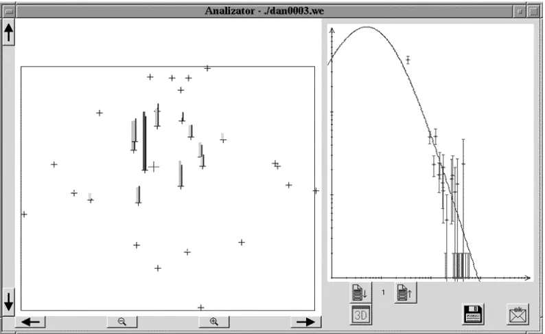
[image:4.595.309.537.608.716.2]Figure 4. The layout of the graphical interface to estimate the EAS parameters using NNN (e.g., ‘by eye’)
as they are given in the second MINUIT column. It is important to note that such ‘bad’ showers of of about 1/3 of all in the 5 x 10¹⁸ eV library.
5. Natural Neural Network Approach
The comparison of ANN and MINUIT methods of shower reconstruction given in the Table 1 shows that the Neural Networks can perform the competitive solutions of the complex minimization problem under study. However, the training procedure of the redundant network takes long and some systematic biases are seen. These are not very strong objections when taking into account the pros. It would be interesting to test the performance of the extremely complex neural network one can imagine, which is, to some extend, the human brain. The training of the brain on a compound problem can be done in principle in two ways. The first one is similar to the ANN training process when the supervising teacher shows the examples of input data and told what the right answer should be. The more effective way is to use the ability of the brain collected in the whole ‘common’ life of the neural net-work as it is.
One can bet that in most cases the ‘usual people’ can react properly seeing the elephant running in their direc-tion (whatever this reacdirec-tion should be) even if they never met an elephant before. The brain (specially human) is so redundant that it can easy adapt the past solution to the new problem. The only requirement needed is that that the new situation must be similar to something seen before. If the similarity is closer than the probability of reaction is expected to be the right one is higher.
We want to use Natural Neural Networks (NNN) to
perform the estimations of the EAS parameters. The problem has to be transformed first to the form which can be understood by the ‘common people’. The knowledge on the elementary particle passing through the atmosphere is helpful in principle, but is useless, in fact, in our case. We would like the NNNs to use their natural abilities.
We have built the graphical interface shown in Figure 4 which contains all what we know and all we should get.
On the left big panel the map of the city is shown in the scale, but without any unimportant information. The map shows position of the detectors (schools) in the Roland Maze Project shower array (the crosses). Next to some schools are the vertical lines (lighter and darker blue and red). The red shows the particle density registered by the detectors (its logarithm, but it is not relevant to the NNNs, and it hasn’t been even told to them). The blue lines show ‘the just proposed’ solution.
The right panel shows, what can be told, the radial dis-tribution of the particle density; horizontally: the distant to the shower axis is given, vertically: the particle den-sity. Points (in red) show the same values as they are on the left plot but ‘the just proposed’ solution is given now by the line (blue).
T. WIBIG 36
adjusted comparing by eye the sizes of the bars of the right plot or/and, what is equivalent, controlling the positions of the points with respect to the curve on the left plot. The ‘user manual’ describing the interface is rather short and simple. The package was supplied with the set of exam-ples showing how the true (known from the simulation)
line should looks like. This explains additionally the task. As the NNN donors we used pupils from the schools collaborating with the Roland Maze Project. They were a little familiar with the problem of EAS, but it was not a requirement, some of them were not. We assumed that each one of our volunteers perform the minimization of 100 showers. The practice shows that after the initial phase one shower takes about 2-5 minutes to be fitted. This gives few hours of the hard work. All NNNs were working on their free time, so we could not motivate them very strongly and there were a number of people which started and never finished the whole task. To avoid boring students we transferred the data to them in packages of 10 and the next 10 can be sent only after receiving the ad-justed previous set. So the whole examining takes usually weeks of work.
The initial position of the shower axis, normalization and age parameters were taken randomly for each new event on display to avoid any unphysical guesses. Results were sent back by e-mail, but the program coded them. It was not possible to see what the numerical value was obtained and to correct them ‘by hand’. The results once sent were put to the database and they couldn’t be changed later on. The error once made remain what sometimes gives strong contribution to overall performance of the particular NNN.
6. Discussion
Anyway, we get some pupils completed their work. We (TW) did it also to be comparing with high school stu-dents’ performance results. In the Table 1 results of TW followed by three (the best) student’s NNNs are given in last four columns.
As it is seen the NNN accuracy is comparable with ANN concerning the shower size estimation (width and the bias), there are also no big differences concerning the axis position. Taking into account that NNN as well as ANN get an answer for each shower it should be com-pared with the ‘all MINUIT’ (third column in the Table 1).
It is interesting to compare results obtained by high school students and TW who can be called a specialist in the field, if not in the shower parameter estimation in general, then at least some specialist, because of building and testing the system of graphic interface etc. In fact
there is no big difference (the sample of only 100 events was used to get the numbers). One can conclude that there is not experience needed.
Insights that the statistics education community badly needs to have, even though it may not know it yet.
Table 2. The improvement (or dis improvement) of the NNN performances concerning the parameter of σN in the course of the EAS analysis
number of analyzed events
10 20 30 40 50 60 70 80 90 100
TW 0.142 0.203 0.199 0.210 0.220 0.239 0.250 0.264 0.261 0.270
NNN
1 0.257 0.237 0.244 0.233 0.235 0.312 0.302 0.291 0.286 0.279 NNN
2 0.379 0.374 0.324 0.307 0.287 0.322 0.305 0.308 0.295 0.294 NNN
3 0.551 0.427 0.390 0.389 0.368 0.363 0.358 0.349 0.335 0.349
It is not obvious, however, when we look how the in-dividual NNN was improving its performance during the process. After analyzing the set of 10 events the results of the accuracy of their estimations were published in the web, and each participant can check how it has gone and what kind of error he made (specially the biases were easy to identify). The ability of the work with the interface could also getting better during the process of using it. Table 2 shows details in the case of the parameter de-scribing the spread of the estimated shower size with respect to the true one. In some cases the improvement
(NNN 3) is seen clearly, while for others (TW) the accu-racy is diminishing with number of analyzed showers. This last is understood, because, in spite of the students, TW has not been limited to analyze only 10 events per day and the last 50 was taken just one by one continuously. The result is surprisingly big. If the constant care could be achieved during all the analysis process it is possible that the result of σN around 0.2. This value is exactly what has been achieved by the trained artificial neural network and significantly better than the standard statistical analysis.
7. Summary
With the help of number of enthusiastic young people we have shown that the redundant Neural Network, Artificial or Natural may work well and in fact in some cases even better than classical statistical tools of minimization. There is the evidence that NNN analyzed in the present work gone even better than the trained ANN. This sug-gests that the further studies of the over-sized networks and their performance are important and the minimization of the network size should not be taken on too early steps of the network arrangement, at least in some cases.
Interest-ing results are expected in the future.
REFERENCES
[1] D. Barnhill, et al., [Pierre Auger Collaboration], Meas-urement of the lateral distribution function of UHECR air showers with the Pierre Auger observatory, Proceedings of the 29th International Cosmic Ray Conference, Pune, India, pp. 101–104; arXiv:astro-ph/0507590, 2005. [2] J. Feder, et al., “The roland maze project: school-based
extensive air shower network,” Nuclear Physics Pro-ceedings Supplements, No. 151, pp. 430–433, 2006. [3] F. James and M. Roos, “Minuit: A system for function
minimization and analysis of the parameter errors and
correlations,” Computer Physics Communications, Vol. 10, pp. 343–367, 1975.
[4] H. O. Klages, et al., “The KASCADE experiment,” Nu-clear Physics Proceedings Supplements, No. 52B, pp. 92– 102, 1997.