Machine learning approaches to exoplanet transit detection and candidate validation in wide field ground based surveys

Machine-learning approaches to exoplanet transit detection and

candidate validation in wide-field ground-based surveys

N. Schanche ,

A. Collier Cameron ,

G. H´ebrard,

L. Nielsen,

A. H. M. J. Triaud,

J. M. Almenara ,

K. A. Alsubai,

D. R. Anderson ,

D. J. Armstrong ,

S. C. C. Barros,

F. Bouchy,

P. Boumis,

D. J. A. Brown ,

F. Faedi,

K. Hay,

L. Hebb,

F. Kiefer,

L. Mancini,

P. F. L. Maxted,

E. Palle,

D. L. Pollacco,

D. Queloz,

B. Smalley ,

S. Udry,

R. West

and P. J. Wheatley

Affiliations are listed at the end of the paper

Accepted 2018 November 13. Received 2018 October 22; in original form 2018 August 15

A B S T R A C T

Since the start of the Wide-angle Search for Planets (WASP) program, more than 160 transiting exoplanets have been discovered in the WASP data. In the past, possible transit-like events identified by the WASP pipeline have been vetted by human inspection to eliminate false alarms and obvious false positives. The goal of this paper is to assess the effectiveness of machine learning as a fast, automated, and reliable means of performing the same functions on ground-based wide-field transit-survey data without human intervention. To this end, we have created training and test data sets made up of stellar light curves showing a variety of signal types including planetary transits, eclipsing binaries, variable stars, and non-periodic signals. We use a combination of machine-learning methods including Random Forest Classifiers (RFCs) and convolutional neural networks (CNNs) to distinguish between the different types of signals. The final algorithms correctly identify planets in the test data∼90 per cent of the time, although each method on its own has a significant fraction of false positives. We find that in practice, a combination of different methods offers the best approach to identifying the most promising exoplanet transit candidates in data from WASP, and by extension similar transit surveys.

Key words: methods: data analysis – methods: statistical – planets and satellites: detection.

1 I N T R O D U C T I O N

Exoplanet transit surveys such as the Convection Rotation and

Plan-etary Transits (Auvergne et al.2009), Hungarian-made Automated

Telescope Network (Hartman et al.2004), HATSouth (Bakos et al.

2013), the Qatar Exoplanet Survey (Alsubai et al.2013), the

Wide-angle Search for Planets (WASP; Pollacco et al.2006), the

Kilo-degree Extremely Little Telescope (Pepper et al.2007), andKepler

(Borucki et al.2010) have been extremely prolific in detecting

ex-oplanets, with over 2900 confirmed transit detections as of 2018

August 9.1

The majority of these surveys employ a system where catalogue-driven photometric extraction is performed on calibrated CCD im-ages to obtain an array of light curves. Following decorrelation of

_{E-mail:[email protected]}

1_{https://exoplanetarchive.ipac.caltech.edu/index.html}

common patterns of systematic error (e.g. Tamuz, Mazeh & Zucker

2005), an algorithm such as the Box Least-Squares (BLS) method

(Kov´acs, Zucker & Mazeh2002) is applied to all of the light curves.

Objects that have signals above a certain threshold are then identi-fied as potential planet candidates. Before a target can be flagged for follow-up observations, the phase-folded light curve is gener-ally inspected by eye to verify that a genuine transit is present. As these surveys contain thousands of objects, the manual component quickly becomes a bottleneck that can slow down the identification of targets. Additionally, even with training it is difficult to establish consistency in the validation process across different observers. It is therefore desirable to design a system that can consistently iden-tify large numbers of targets more quickly and accurately than the current method.

Several different techniques have been used to try to automate the process of planet detection. A common method is to apply thresholds to a variety of different data properties such as signal-to-noise ratio, stellar magnitude, number of observed transits, or

2018 The Author(s)

measures of confidence of the signal, with items exceeding the given threshold being flagged for additional study (for WASP-specific

examples, see Christian et al.2006; Gaidos et al.2014). Applying

these criteria can be a fast and efficient way to find specific types of planets quickly, but they are not ideal for finding subtle signals that cover a wide range of system architectures.

Machine learning has quickly been adopted as an effective and fast tool for many different learning tasks, from sound recognition

to medicine (see e.g. Lecun, Bengio & Hinton2015, for a review).

Recently, several groups have begun to use machine learning for the task of finding patterns in astronomical data, from identifying

red giant stars in asteroseismic data (Hon, Stello & Yu2017) to

using photometric data to identify quasars (Carrasco et al.2015),

pulsars (Zhu et al.2014), variable stars (Dubath et al.2011;

Rimol-dini et al.2012; Masci et al.2014; Naul et al.2017; Pashchenko,

Sokolovsky & Gavras2018), and supernovae (du Buisson et al.

2015). For exoplanet detection in particular, Random Forest

Clas-sifiers (RFCs; McCauliff et al. 2015; Mislis et al. 2016),

artifi-cial neural networks (ANNs; Kipping & Lam2017), convolutional

neural networks (CNNs; Shallue & Vanderburg2018), and

Self-Organizing Maps (Armstrong, Pollacco & Santerne 2017) have

been used onKeplerarchival data. CNNs were trained on simulated

Keplerdata by Pearson, Palafox & Griffith (2018).

WhileKeplerprovides an excellent data source for machine

learn-ing (regular observations, no atmospheric scatter, excellent preci-sion, large sample size), similar techniques can also be applied to ground-based surveys, and in fact machine-learning techniques have recently been incorporated by the MEarth project (Dittmann et al.

2017) and NGTS (Armstrong et al.2018). We extend this work by

applying several machine-learning methods to the WASP data base. In Section 2, we briefly describe the current process for WASP candidate evaluation. Then in Section 3, we discuss the methods developed, focusing on RFC and CNN, and describe how these methods are applied to data from the WASP telescopes. In Sec-tion 4, we discuss the efficacy of the machine-learning approach, with an emphasis on the false-positive candidate identification rate. Finally, in Sections 5 and 6, we discuss practical applications of the machine classifications in the future follow-up of planetary candidates.

2 O B S E RVAT I O N S

For this work, we focus entirely on WASP data, although similar techniques would be applicable to any ground-based wide-field

tran-sit survey. The WASP project (Pollacco et al.2006) consists of two

robotic instruments, one in La Palma and the other in South Africa. The project was designed using existing commercial components to reduce costs, so each location is made up of eight commercial cam-eras mounted together and using science-grade CCDs for imaging. The WASP field is comprised of tiles on the sky corresponding

approximately to the 7.8 deg2_{field of view of a single WASP}

cam-era. The WASP data base includes data on all objects in the tiles secured over all observing seasons in which the field was observed. Decorrelation of common patterns of systematic error has been carried out using a combination of the Trend Filtering Algorithm

(TFA; Kov´acs, Bakos & Noyes2005) and the SysRem algorithm

(Tamuz et al.2005). Initial data reduction was carried out

season-by-season and camera-by-camera. More recently, re-reduction with the ORCA TAMTFA (ORion transit search Combining All data on a given target with TAMuz and TFA decorrelation) method has yielded high-quality final light curves for all WASP targets. Each tile typically contains between 10 000 and 30 000 observations.

In total, there are 716 ORCA TAMTFA fields, with each field containing up to 1000 tentative candidates identified as showing BLS signals above set thresholds in antitransit ratio and

signal-to-red-noise ratio (see Collier Cameron et al.2006for details).

At this point in the process, WASP targets are selected for follow-up by a team of human observers. The observers can either look at light curves by field or can apply filters, cutting on thresholds for selected candidate properties. Finding these cuts has been done through trial and error, and can vary between observers. The targets of interest are prioritized for radial velocity or photometric follow-up observations. Only after successful secondary observations can an object be identified as a planet in the data base. However, both the vetters and the follow-up observers can flag the star as something else, such as an eclipsing binary, stellar blend, or variable star before or after follow-up observations confirm the source, which makes misclassifications of these object types possible. The final catego-rization (planet, eclipsing binary, variable, blend, etc.) recorded by human vetters or observers is known as the disposition.

While effort was taken early in the WASP project to standard-ize individual classifications through training sessions and cross-validation, the current method of identifying planetary candidates remains partially dependent on individual opinions. It would be bet-ter to establish a system that can systematically go through all of the data and identify targets, ideally ranked by their likelihood to be genuine planets, derived from the knowledge gained from the entire history of past dispositions. The past decade of classifications and observations has generated a data set containing both descriptions of the target and their classification, creating an excellent starting point for supervised machine learning.

3 M E T H O D S

Several classification algorithms were explored with the goal of reliably identifying planet candidates. We seek to more efficiently use the telescope time for follow-up observations by reducing the number of false-positive detections as far as is reasonable without compromising sensitivity to rare classes of planet such as short-period and inflated hot Jupiters. Other goals, such as finding specific subsets of planets with higher precision, could be carried out by retraining the algorithms for that given purpose. In this section, we will discuss the different machine-learning methods utilized and the data sets created to train the algorithms.

3.1 Initial data exploration

Periodic signals in the light curve can come from astrophysical

sources other than transiting planets (Brown 2003). We refer to

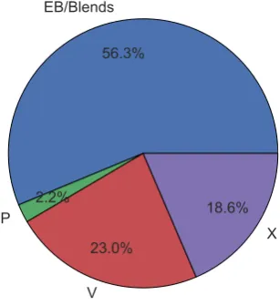
a periodic dip caused by something other than a planet as an as-trophysical false positive. It is essential for any machine-learning application to distinguish between planetary signals and false posi-tives. Fortunately many types of astrophysical configurations have been identified in the WASP archive. The training data set used for the RFC is composed of a table of data containing all of the planets (P), eclipsing binaries, both on their own and blended with other nearby objects (EB/Blend), variable stars (V), and light curves containing no planetary transit after human inspection (X). Blends are especially common in WASP data because it has a 3.5 pixel (48 arcsec) aperture, leading to the blending of signals from several stars. It is notable that the WASP archive labels a planet as ‘P’ even if discovered by a different survey. While not all of these plan-ets are detectable by eye in the WASP data, planplan-ets discovered by other instruments are included in the training sample with the aim

Figure 1. Pie plot showing the relative number of examples for planets (P), eclipsing binaries and blends (EB/Blends), variable stars (V), and light curves otherwise rejected as planet hosts (X). This represents an unbalanced data set, with the smallest class being the class of special interest, planets. In real life, there are more non-detections (X) than the other classes. However, the training data is composed of light curves that have been manually iden-tified and flagged. Many non-detections are simply ignored by observers rather than labelled X, leading this class to be smaller than expected. The mismatched sample size is important in machine learning, as considerations must be taken to bring representation to the minority classes.

of extending the parameter space to which the classifiers are sensi-tive. Low-mass eclipsing binaries (EBLMs) were excluded from the training and testing data sets, as their signals look photometrically similar to that of a transiting planet. However, we do test the final algorithms performance on these objects in Section 4.

The final size of each of these classes is shown in Fig.1. All light

curves used in this study have been classified by members of the WASP team as of 2018 August 6 and have a V-magnitude of less than 12.5. We used only the amalgamated light curves combined across all cameras and observing seasons for which data was present that were then de-trended with a combination of SysRem (Tamuz

et al.2005) and the TFA (Kov´acs et al.2005) and searched with a

hybrid BLS method (Kov´acs et al.2002).

An initial transit width, depth, period, epoch of mid-transit, and radius are estimated from the BLS. Stellar features such as the mass, radius, and effective temperature are found by the method

described by Collier Cameron et al. (2007), in which the effective

temperature is estimated from a linear fit to the 2MASSJ− H

colour index. The main-sequence radius is derived fromTeffusing

the polynomial relation of Gray (1992), and the mass follows from

a power-law approximation to the main-sequence mass–radius

rela-tion,M∗∝R1/0.8

∗ . A more rigorous fit to the transit profile yields the

impact parameter and the ratio of the stellar radius to the orbital sep-aration, and hence an estimate of the stellar density. Markov-chain Monte Carlo (MCMC) runs are performed to sample the posterior probability distributions of the stellar and planetary radii and orbital inclination. The MCMC scheme uses optional Bayesian priors to impose a main-sequence mass and radius appropriate to the stellar effective temperature. Note that the results and predictions would change if the precise radius were used instead, particularly if the star has evolved off of the main sequence (MS).

In addition to the provided information, we add several new fea-tures to capture more abstract or relational information, such as the ratio of transit depth to width and the skewness of the distribution of the magnitudes found within the transit event. The latter is a

pos-sible discriminator between ‘U’ shaped central transits of a small planet across a much larger star, and shallow ‘V’ shaped eclipses of grazing stellar binaries. The new high precision distance

calcula-tions released byGaia(Gaia Collaboration2016,2018) are used to

measure the deviation of the estimated main-sequence radius cal-culated as above and the measured radius. In total, 34 features are included in the data set. A full list of features and their definitions

can be found in Table1.

Before training, the full data set containing the star name, de-scriptive features, and disposition is split randomly into a training data set and a test data set. In total, there are 4697 training cases and 2314 testing samples. Prior to running the classifiers, all of the features of the training data set are median centred and scaled in order to reduce the dynamic range of individual features and to improve performance of the classifier. The scaling parameters are retained so that they can be applied to subsequent data sets to which the classification is applied, including the testing data set.

The training data set is used as an input to a variety of classi-fiers, namely a Support Vector Classifier (SVC; Cortes & Vapnik

1995), Linear Support Vector Classifier (LinearSVC), Logistic

re-gression (for the implementation inSCIKIT-LEARN, see Yu, Huang &

Lin2011), K-nearest neighbours (KNN; Cover & Hart1967), and

RFC (Breiman2001). All of the classifiers are run using the

rele-vant functions in Python’sSCIKIT-LEARNpackage (Pedregosa et al.

2011). The classification algorithms have default tuning parameters,

but they are not always the best choice for the given data set. We therefore vary the parameters in order to find an optimal combina-tion. While it is impractical to test every possible combination of parameters, we ran a grid of tuning parameter combinations specific to each classification method to find the optimal settings for the fi-nal algorithm. The results using the best performing parameters for

each method are reported in Table2. A more detailed description

of what each parameter does can be found in the documentation for SCIKIT-LEARN.2

Several of the classifiers, and particularly the KNN classifier, show poor performance using the training data because the class of interest, the planets, is under-represented in the data set. To try to compensate for this, we also try adding additional data points using the Synthetic Minority Over-sampling Technique (SMOTE;

Chawla et al.2002). This technique creates synthetic data points for

the minority classes that lie between existing data points with some added random variation. The synthetic data is added only to the training data, and the test data set remains the same as before. The addition of SMOTE data generally increased the number of planets retrieved from the data, but also increased the number of non-planets given a planet classification. The exception is the SVC, which shows a sharp decrease in false positives while the true positives and true negatives remain the same.

3.2 Random Forest Classifiers

After exploring several different classification techniques, we de-cided to pursue the RFC in more detail because of its high recall rate

(see Table2). RFC is one of the most widely used machine-learning

techniques, and is particularly useful in separating data into spe-cific, known classes. Applications to astronomy include tracking the different stages of individual galactic black hole X-ray binaries

by classifying subsections of the data (Huppenkothen et al.2017),

classifying the source of X-ray emissions (Lo et al. 2014), and

2_{http://scikit-learn.org/stable/}

Table 1. Features used by the classifiers. Starred features are those added to the data set, while the rest were taken directly from the Hunter query. The efficacy of many of these measures for false-positive identification is discussed in detail by Collier Cameron et al. (2006).

Feature name Description

clump idx Measure of the number of other objects in the same field with similar period and epoch. dchi P∗ Theχ2_{value at the best-fitting period from the BLS method.}

dchi P vs med∗ The ratio ofχ2_{at the best-fitting period to median value.}

dchisq mr Measure of the change in theχ2_{when MCMC algorithm imposes a MS prior for mass and radius.}

delta Gaia∗ Stellar radius from MCMC –GaiaDR2 radius divided byGaiaDR2 radius. delta m∗ The difference between the mass calculated byJ−Hand the MCMC mass. delta r∗ The difference between the radius calculated byJ−Hand the MCMC mass. depth The depth of the predicted transit from Hunter.

depth to width∗ Ratio of the Hunter depth and width measures.

epoch Epoch of the predicted transit from Hunter (HJD-2450000.0). impact par Impact parameter estimated from MCMC algorithm. jmag-hmag Colour index,Jmagnitude –Hmagnitude.

kurtosis∗ Measure of the shape of the dip for in-transit data points. mstar jh Mass of the star, from theJ−Hradius∗(1/0.8). mstar mcmc Stellar mass determined from MCMC analysis.

near int∗ Measure of nearness to integer day periods, abs(mod(P+0.5,1.0)−0.5). npts good Number of good points in the given light curve.

npts intrans Number of data points that occur inside the transit.

ntrans Number of observed transits.

period Detected period by Hunter? in seconds.

rm ratio∗ Ratio of the MCMC derived stellar radius to mass. rplanet mcmc Radius of the planet, from MCMC analysis.

rpmj Reduced proper motion in theJband (RPMJ=Jmag+5∗log10(mu)). rpmj diff Distance from DWs curve separating giants from dwarfs.

rstar jh Radius of the star derived from theJ−Hcolour measure. rstar mcmc Radius of the star determined from MCMC analysis.

sde Signal detection efficiency from the BLS.

skewness∗ Measure of the asymmetry of the flux distribution of data points in transit. sn ellipse Signal to noise of the ellipsoidal variation.

sn red Signal to red noise.

teff jh Stellar effective temperature, fromJ−Hcolour measure.

trans ratio Measure of the quality of data points (data points in transit/total good points)/transit width.

vmag Catalogued V-magnitude.

width Width of the determined transit in hours.

Table 2. Results of the classification algorithms, trained on 4697 samples. The results here are reported for the 2314 samples making up the test data set. We report here the planets correctly identified (True Positives – TP), non-planets incorrectly labelled as planets (False Positives – FP), and the num-ber of planets missed by the algorithm (False Negative – FN). From this we calculate the precision [TP/(TP+FP)], recall [TP/(TP+FN)], andF1 score [F1=2∗Precision∗Recall/(Precision +Recall)] for the planets. The accuracy reflects the performance of the classifier as whole, and shows the total number of correct predictions of any label divided by the total number of samples in the test data set. The full confusion matrix for all of the classifiers reported here can be found as an appendix in the online journal. The tuned parameters column reports the best performing values for the listed parameters, as determined by using the GridSearchCV function, which tests all combinations of a specified grid of parameters. Classifiers marked with an∗use a training sample that added training examples using SMOTE sampling, explained more fully in the text. By adding SMOTE data points, the training set grew to 10 672 samples, while the testing data set remained the same. The LinearSVC, SVC, and Logistic Regression Classifier that did not use the SMOTE data points are run using the keyword class weight=‘balanced’, which weights each sample based on the number of entries in the training data set with that label. The RFC without SMOTE resampling uses the class weight keyword ‘balanced subsample’, which has the same function but is recomputed for each bootstrapped subsample. While the SVC both with and without the SMOTE training sample performed very well in the ‘F1’ score and overall accuracy, the false-negative rate was higher than desired for practical application. The RFC showed the highest recall, which we want to maximize to find the widest range of planets. We therefore prefer the RFC, with a trade-off of having more false positives that would be flagged for follow-up.

Classifier TP FP FN Precision Recall F1 Accuracy Tuned parameters

LinearSVC 35 83 13 30 73 43 80 C=60, tol=0.0005

SVC 37 46 11 45 77 57 82 kernel=‘rbf’, C=12, gamma=0.03

LogisticRegression 34 76 14 31 71 43 81 C=90, tol=0.005

KNN 5 4 43 56 10 17 81 n neighbors=15, weights=‘distance’

RandomForest 44 125 4 26 92 41 79 n estimators=200, max features=6, max depth=6

LinearSVC∗ 44 142 4 24 92 38 76 C=20, tol=0.0002

SVC∗ 36 37 12 49 75 59 81 kernel=‘rbf’, C=25, gamma=0.02

LogisticRegression∗ 42 128 6 25 88 39 78 C=60, tol=0.0006

KNN∗ 45 151 3 23 94 37 74 n neighbors=7, weights=‘distance’

RandomForest∗ 45 137 3 25 94 39 78 n estimators=200, max features=6, max depth=6

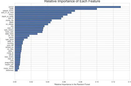
Figure 2. Ranked list of the effectiveness of each of the features in making correct classifications of the training data set for the RFC. Properties of the transit itself, such as the period and width, are shown to be important discriminators in identifying genuine transits, while stellar properties like magnitude and mass are not effective for classification.

distinguishing between types of periodic variable stars (Rimoldini

et al.2012; Masci et al.2014)

RFC has many advantages, most notably the ease of implemen-tation, solid performance in a variety of applications, and most im-portantly for our study, the easily traceable decision processes and feature ranking. It is because of this last advantage that we focus our attention on the RFC over the LinearSVC, SVC, linear regression, or KNN methods. RFC is an ensemble method of machine learning, comprised of several individual decision trees. Each decision tree is trained on a random subset of the full training data set. For each ‘branch’ in the tree, a random subset of the input characteristics known as ‘features’ are selected and a split is made based on a given measure that maximizes correct classifications, with samples falling above and below the split point moving to different branches. Each branch then splits again based on a different random subsam-ple of features. This continues until either all remaining items in the branch are of the same classification or until a specified limit is reached. The output of the RFC is a fractional likelihood that the input object falls into each category, and the highest likelihood is then used as the classification.

On its own, each decision tree does not generalize well to other data sets to make predictions. However, by training many different trees and combining them to use the most popular vote as the predic-tion, a more successful and generalized predictor is created. There are many ways to tune the RFC to try to optimize the classification for the data set. For example, the number of trees in the forest, the depth of the tree (the number of splits that can be performed), the number of features available at each split, and the method used to optimize the splits are all characteristics that can be modified. There is no set rule for choosing these parameters, and therefore many dif-ferent tests are conducted to try to optimize the results. Here, we

useSCIKIT-LEARN’SRFC method to perform the classification and to tune the parameters. We find that the highest performing forest contains 200 trees, above which the accuracy increased very mini-mally for the increased computation time. Each tree was capped at a depth of 6 and allowed six random features at each split in the tree, which helps to reduce overfitting.

One advantage of the RFC method is that many different features can be included, and not all features need to be effective predictors. This can be useful for exploratory data analysis as the user can include all of the various data elements without introducing biases from curating the input list. Conversely, it is important to note that the performance of the RFC depends on the quality of the input features. It is possible that the performance of all classifiers could increase if better features are identified.

As a byproduct of the training process, the RFC can analyse the importance of the various features in making predictions. The results

of such an analysis using our training data set are shown in Fig.2.

This can be used to gain insight into the decision making process that the classifier has developed, which can inform further analysis. For example, the period of the planet was the strongest indicator. This can be explained in large part because false planet detections arising from diurnal systematics tend to have orbital periods close to multiples of one sidereal day due to the day/night cycle present in Earth-based observations. This indicator would likely not play as significant a role in a space-based survey unaffected by the day/night cycle. The width or duration of the transit, estimated radius of the

planet, theχ2_{value (a product of the BLS search) of the object}

at the best-fitting period, and the number of transits of the object round out the top five features in prediction.

The features that had relatively little impact on the overall pre-diction related largely to stellar properties, including the magnitude

Figure 3. Confusion matrix showing the results of the RFC using the training data set containing synthetic data points generated through SMOTE sampling. Thex-axis indicated what the algorithm predicted and they-axis displays the human labelled class, which we assume to be accurate. Correct predictions fall on a diagonal line from upper left to lower right. The plot on the left shows the results as a fraction of light curves that fall into that bin. However, since the number of samples in each class varies, a more practical depiction is shown in the right plot, which shows the actual number of light curves for each category. and radius of the star. This shows that there is no strong preference

for a certain size star to host a particular type of object in our sample, as the apparent magnitude range to which WASP is most sensitive

is dominated by F and G stars (Bentley2009). The lowest ranked

feature is the skewness, showing that the asymmetry of data points falling within the best-fitting transit is not sufficiently capturing the transit shape information.

The results of the RFC, shown in Fig.3, show that∼93 per cent of

confirmed planets are recovered from the data set. The ones that are not recovered are most often rejected with the label ‘X’. The more concerning statistic is that more than 10 per cent of EB/Blends were misclassified as planets. Since there are far more binary systems recorded than there are planets, this quickly turns into a large number of light curves incorrectly identified, which translates to many hours of wasted follow-up time. For our testing data set, there are 45 correct planet identifications and 137 that are false positives. This means that if all objects flagged as planets are followed up on, we would expect about 25 per cent of them to be planets. In reality, not all flagged objects are good candidates and can be eliminated by visual inspection. Regardless, the high false-positive rate led to the development of CNNs as a secondary test on the light curves, as discussed in 3.3.1.

3.3 Neural networks

The past decade has shown an explosion of new applications of neu-ral networks to tackle a variety of different problems. The particular flavor of neural networks is dependent on the specified task at hand and the types of data available for training. The basic idea of a neural network was originally inspired by the neurons in a human brain, although in practice artificial neurons are not directly analogous. None the less, like the human brain, this type of structure is useful for learning complex or abstract information with little guidance from external sources. In the following section, we discuss CNNs and their application to the WASP data base.

3.3.1 Convolutional neural networks

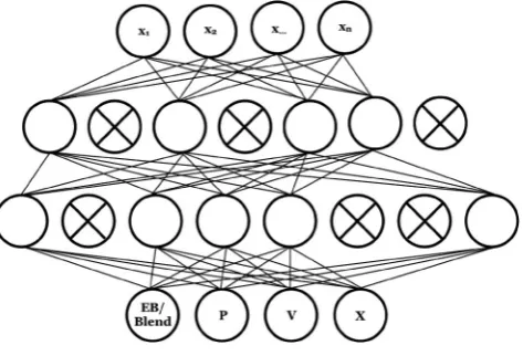
A standard ANN has the basic structure of an input layer containing the features of the input data, one or more hidden layers where

Figure 4. Visual representation of a neural network scheme, where circles represent individual neurons. In this example, the layers progress from top to bottom. The top row represents the input layer, followed by two hidden layers, and finally an output layer, where the class prediction is made. Circles with crosses through them represent dropped neurons, described further in the text.

transformations are made, and the output layer which offers the classification. The output of each layer is transformed by a non-linear activation function. The basic building-blocks of ANNs are known as neurons. A basic schematic of the system architecture is

shown in Fig.4.

In this work, we use theKERASpackage (Chollet et al. 2015)

to implement the neural network, which offers a variety of built-in methods to customize the network. At each layer, the input data is passed through a non-linear activation function. Many activation function choices are available, but here we choose the rectified linear

unit, or ‘relu’ function (Nair & Hinton2010) for all layers except

the output layer, to which we instead apply a sigmoid function. The relu function was chosen both because of its wide use in many applications and because of its high performance during a grid search over our tuning parameters. In addition to the activation function, each neuron is assigned a weight that is applied to the output of each layer, and is modified as the algorithm learns. Using KERAS, we tested a random normal, a truncated normal distribution

within limits as specified by LeCun (LeCun et al.1998), and a

uniform distribution within limits specified by He (He et al.2015)

initialization of the weights and found the greatest performance with He uniform variance scaling initializer.

The learning itself is managed using the Adamax optimizer

(Kingma & Ba2014), a method of optimizing gradient descent.

In gradient descent, classification errors in the final output layer are propagated backwards through the network and the weights are adjusted to improve the overall error during the next pass through the network. This is an iterative process, with small adjustments made after each pass through the network until a minimum er-ror (or maximum number of iterations) is reached. The maximum change in the weights allowed by Adamax at each iteration is con-trolled by the learning rate, which can be tuned to different val-ues for individual data sets. Finally, at each stage, we incorporate neuron dropouts, where a fraction of the neuron inputs are set to 0 in order to help prevent overfitting. The total dropout per cent is determined experimentally, and here we find 40 per cent to be effective.

While the numerical data used in the RF could be passed to the neural network directly, this data only provides insight into the sta-tistical distribution of the classes, producing results similar to that of the RFC. In practice, it can be the case that many of the features fall within the right range to be labelled with a certain class, but a quick visual inspection of the light curve can easily rule the clas-sification out. Instead, it would be desirable to create an algorithm that can use the shape of the light curve itself to make classification decisions. Using the light-curve data would more closely mimic the human process of eyeballing.

In order to directly use the light-curve data, we developed a CNN

(LeCun et al.1990; Krizhevsky, Sutskever & Hinton2012). In this

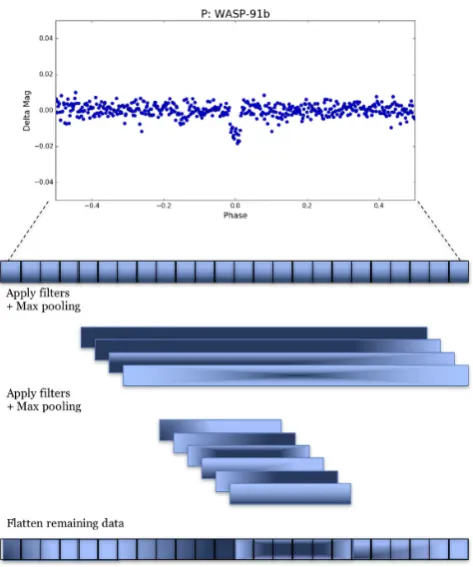
case, the input data we use is the actual magnitude measurements of WASP folded on the best-fitting period determined by the BLS. In the CNN that we adopt, the magnitude data first undergoes a series of convolution steps, in which various filters are applied to the data to enhance defining characteristics and detect abstracted features. The filters themselves are optimized iteratively to find those that best enhance the differences between classes, similar to the way the weights between the neural layers are updated. The convolution

process is represented in Fig.5.

Each WASP field contains a different number of sample points, yet input to the CNN for all of the samples need to be of the same length. To standardize the data length, the folded light curves are divided into 500 bins in transit-phase space. The number of bins was determined experimentally, with 500 being the best trade-off between providing detailed light curves without having a significant number of bins missing data.

Once the data are binned, a set of one-dimensional convolution filters are passed over each light curve. This has the effect of making our data set larger by a factor of the number of filters, so to reduce the data size and help prevent overfitting we apply a MaxPooling

layer where we only keep the maximum value of everyn data

points. Finally a dropout layer is added, in which a random specified fraction of the points are ignored to prevent overfitting the training data. We then repeat this entire process to add more complex and abstract filters. Finally, all of the remaining data is flattened so that each light curve, now comprised of several filtered and pooled representations of the original light curve, are added together to make a one-dimensional array for each star, which is then passed into the fully connected layers of the neural network. All of the layers of the network are optimized to provide the best fit to the data in the final classification layer.

Figure 5. Simplified visual representation of the convolution steps for a full light curve, folded on the best-fitting period. The shading of the boxes represents the different filters that are applied to the data in each step. Also at each convolution step, the data length is reduced using the Max Pooling method, in which only the maximum value of everyndata points is kept. In the final step, all of the pooled and filtered data are stacked one after the next. This new one-dimensional data set is then passed into the fully connected layers of the neural network. The final network architecture is as follows: the input data is comprised of one-dimensional magnitude data binned to length 500. The first convolution step has eight filters with a kernel size of 4. The data is then pooled by 2. Each light curve at this point has eight layers of length 250. The second convolution step has 10 filters with a kernel size of 8, followed again by another pooling layer with a pool size of 2 leading to a data size of 10 layers of length 125. The information from all of the filters is then flattened into one layer of length 1250 for each light curve, and is input to the first densely connected layer. There are two dense hidden layers of size 512 and 1024. Each stage of the convolution and fully connected layers has a 40 per cent dropout rate to prevent overfitting. The final output layer has four neurons, one for each classification category. The CNN with both the full and local light curve has the same general format, but with the input data being a stack of two 500-length light curves.

The training set is highly unbalanced with relatively few planets as compared to eclipsing binaries and blends, variables, or light curves with no signal, which limits the performance of the CNN. To compensate, we extended the sample of ‘P’ training examples by creating artificial transit light curves.

The light-curve injection was done by adding synthetic transit signals to existing WASP light curves that showed no transit signal or other variability. This ensured realistic sampling and typical pat-terns of correlated and uncorrelated noise. We began with a sample of light curves of objects classified as ‘X’ in the Hunter catalogue, meaning they have been rejected and contain no detectable planet signal. We started with all X stars and measured the RMS against

the V-magnitude. Those objects that fell more than 1σ below the

best fit to the data were selected, as they show the least amount of variation. This left a total of 848 light curves.

The planetary signal added to the WASP data was created using the BATMAN package forPYTHON (Kreidberg2015). The stellar mass, radius, and effective temperature are set using the known values for the star itself. The planetary properties were generated randomly with the following distributions.

The period was randomly selected to be a value uniformly located in log space between 0.5 and 12 d, as this is the range in which the WASP pipeline typically uses the BLS algorithm to look for planets. The mass of the planet follows the same lognormal distribution used

in Cameron & Jardine (2018), with a mean of 0.046 and a sigma

value of 0.315. The semimajor axis can be found for the period using

a=(p 2_G(M

1+M2)

4π2 )

1

3 ₍₁₎

The radius of the planet is dependent on both the mass of the planet and the equilibrium temperature. We use a cubic polynomial in log mass and a linear term in log effective temperature to approximate the planetary radius, using coefficients derived from a fit to the

sample of hot Jupiters studied by Cameron & Jardine (2018):

log

Rp

RJup

=c0+c1log

Mp

0.94MJup

+c2log

Mp

0.94MJup

2

+c3log

Mp

0.94MJup

3

+c4log

Teql 1471 K

4

, (2)

wherec0=0.1195,C1= −0.0577,c2= −0.1954,c3=0.1188,

c4=0.5223, andTeql=Teff

RS

2a 1

2_.

As we are looking only for close-in planets, we make the sim-plification that all eccentricities are 0. Finally, the inclination was

calculated by first randomly picking an impact parameter,b,

be-tween 0 and 1. The inclination was then calculated by

i=cos−1

bRS

a

. (3)

The light curves were generated and added to one of the selected WASP light curves folded on the assigned period. While some of these new planets were too small to be visible, and others were much larger than would be expected, we chose to include them all in order to push the boundaries of the parameter space that the CNN is sensitive to so as not to exclude potentially interesting, though unusual, objects.

The light curves of the artificial planets, as well as real-data ex-amples of P’s, EB/Blend’s, V’s, and X’s are phase folded on the best-fitting period (or assigned period, in the case of the artificial planets) and binned by equal phase increments. Including the arti-ficial planets, there are 4627 objects in the training set and 2280 in the testing data set.

The CNN parameters were set by using a grid search over the tunable parameters. The final CNN was comprised of two convolu-tional layers with 8 and 10 filters, respectively. The pooling stages each had a size of 2, and 40 per cent of the neurons were dropped at each set. The flattened data were passed to a neural network with two hidden layers of sizes 512 and 1048 and with a ‘relu’ function. Both of these layers also had a 40 per cent dropout applied. The learning rate for the Adamax optimizer was 0.001. The most effec-tive batch size was 20 with 225 total epochs. As with the RFC, the output of the CNN is a likelihood that the light curve falls into each of the categories, with the highest likelihood being the prediction.

Using only the binned light curve as input, the CNN achieves an overall accuracy (correct predictions divided by total light curves analysed) of around 82 per cent when applied to the test data set.

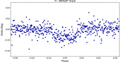
Figure 6. A local view of WASP-91b, the same planet as shown in the CNN example (Fig.5). This local view was used as an additional layer in the second CNN. The local version clearly shows more detail on the transit shape, and specifically the flat-bottomed transit. EB/Blends tend to have a ‘V’ shape with steeper sides, which is more apparent in this close-up view.

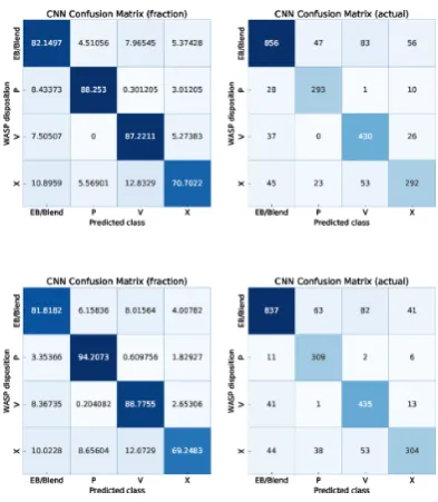
While the fraction of correctly identified planets is lower than the RF (88 per cent as opposed to 94 per cent), the CNN performs much better in classifying eclipsing binaries and blends in terms of

the per cent of false positives with only∼5 per cent of EB/Blends

being labelled as planets, as opposed to 10 per cent for the RF. The CNN therefore has an overall better performance for follow-up efficiency.

In order to further increase the performance of the CNN, we train a second CNN algorithm to include the local transit information,

using an approach similar to that of Shallue & Vanderburg (2018).

The local information is comprised of the data centred on the transit and only containing the data 1.5 transit durations before and after the transit event, standardizing the transit width across events. An

example of a local light curve is shown in Fig. 6. The effect of

this is to provide greater detail and emphasis on the shape of the transit event itself in order to understand the subtle shape difference between a typical planet and an eclipsing binary system. The full light curve and the local view are stacked and passed together into the CNN. In this case, the overall accuracy (83 per cent) remained roughly the same, but the totalpercentage of planets found increased to (94 per cent). The trade-off is a slight increase of the number of EB/Blends being labelled as planets. A full comparison of both

methods can be seen in Fig.7.

It is important to note that the way missing data was handled for both the full light curve and the local light curve made a large difference in the final performance. When binning the data, the full data set was evenly split in 500 equal phase steps and all of the data points within those phase steps were averaged. In some cases, for example when the light curve was folded over an integer day, there were gaps in the phase ranges in which no data were present. Since the CNN cannot handle missing data in the input string, a value needs to be inserted. We tried inserting either a nonsense value, in this case 0.1 which is far above any real data point, or repeating the last good value. In some cases there were several phase steps in a row that were missing data, causing a small section of the light curve to be flat.

After trying both options, we found that by far the best perfor-mance was obtained when inserting the nonsense value into the full light curve and repeating the last good value into the local light curve. This makes sense, as the full light curve gives a broader view of the star’s light curve and is likely to have regular gaps in the data when it is folded on a bad period. The algorithm was able to iden-tify that pattern and reject it. The local data, however, have fewer total data points because they cover a smaller total range of phases, and therefore are more likely to randomly have missing data. The

Figure 7. Confusion matrix showing the results of the CNN using only light curves folded on the best-fitting period (top) and with the addition of the local transit information (bottom) as input. The axes are interpreted the same as in Fig.3. The plot on the left shows the results as a fraction of light curves that fall into that bin. The right plot shows the actual number of light curves for each category. Note that in this example, we artificially injected additional planets into WASP data to increase the sample, so the numbers reported are for a combination of the real and artificial planets.

algorithm is no longer able to distinguish light curves missing data because of an intrinsic problem with the data fold and those miss-ing data simply because they lack enough observations durmiss-ing the transit, confusing the results.

4 A N A LY S I S A N D R E S U LT S

When looking at the results of the RFC and CNNs, the percentage of

correct predictions across methods is consistent, with∼90 per cent

of planets being correctly identified. However, when looking at the original light curves for both true positives and false negatives, clear patterns in the different machine-learning methods begin to emerge. The RFC uses features that are derived from the fitted light-curve parameters and external catalogue information, but the light curves themselves are not included. This logically leads to candidates that have typical characteristics of known exoplanets to emerge. How-ever, because the WASP data can be very noisy and have large data gaps, there are many occasions where the derived ‘best-fitting’ planet features fall into the known distribution, but upon inspecting the original data it is clear that there is no periodic transiting signal. Examples of true-positive and false-negative classifications for the

RFC are shown in Fig.8. The main contributors of false positives

for the RF is the blended star (rather than the eclipsing binary) com-ponent of the EB/Blends. In many cases, the blended stars look very similar to planets by their numerical descriptors, and in particular the depth of the transit and the distribution of transit durations look very plausible. Without looking at the nearby stars, these objects are very hard to distinguish.

The CNN has a fundamentally different method of identifying transits. As described in Section 3.3.1, the CNN is not provided with derived data, but rather has direct access to the magnitude data folded on the best-fitting period. In this case, the algorithm

is simply trying to pattern-match to find the correct shape for a transit. Looking at the true positives and false negatives (examples

shown in Fig.9) for this subsection of data shows a different failure

mechanism for wrongly identified planets. In many cases, light curves will look like planets, but when other information, such as the depth of the transit, is known it becomes clear that the object is more likely an eclipsing binary or other false positive. In addition, fainter objects tend to have much noisier data and more sporadic signals, which can sometimes look like a transit signal when the data is binned down to 500 data points. Finally, the drift of stars across the CCD during each night can lead to systematic disturbances that are consistent at the beginning or end of each night in some (but not all) target stars. Since this effect is specific to each star, it is not always corrected by decorrelation. This can lead to the light curve having a clear drop in magnitude at regular intervals, and the gaps in the data can appear transit-like to the CNN. Interestingly, this last problem is far more prevalent when fewer neurons in the ANN are used. Increasing the neurons to 512 and 1024 in our final configuration nearly eliminates the problem, although a few cases do still get through.

5 D I S C U S S I O N

Each of the machine-learning methods above performs best on a specific subset of planets. Like a human looking at a list of transit properties, the RFC and SVC are better suited to finding planets that have strong signals and have properties similar to those of the other known WASP planets. The CNN using the magnitude data folded on the best-fitting period functions similar to a human eyeballing a light curve and making decisions. By combining the predictions of these methods, we get a more robust list of planetary candidates. The importance of the combination of machine-learning algorithms

has also been noted by others (Morii et al. 2016; D’Isanto et al.

2016), and will be an important framework for upcoming large-data

surveys.

Currently, radial velocity follow-up of WASP targets takes place primarily using the CORALIE spectrograph at the La Silla

Obser-vatory in Chile (Queloz et al.2000) for southern targets and the

Spectrographe pour l’Observation des Ph´enom`enes des Int´erieurs

stellaires et des Exoplan`etes (SOPHIE; Perruchot et al. 2011) at

the Haute-Provence Observatory located in France for targets in the north.

Since thorough records have been kept of the WASP follow-up program with CORALIE, 1234 candidates have been observed and dispositioned. Of those, 150 (12 per cent) have been classified as planets (2 of which are the brown dwarfs 30 and WASP-128), 713 (58 per cent) are binaries or blends, 225 (18 per cent) were EBLM, and the remaining 146 (12 per cent) were rejected for other reasons, including 60 because the stars turned out to be inflated giants. The SOPHIE follow-up effort has a similar success rate to date. Of the 568 total candidates dispositioned, 53 (9 per cent) are planets, 323 (57 per cent) are blends or binaries, 116 (20 per cent) were EBLM, 72 (13 per cent) were rejected for other reasons in-cluding being a giant star, and 4 (1 per cent) were variable stars.

As a comparison, for our RFC, 182 objects were classified as planets, with 45 true positives and 137 false positives, indicating a success rate of 25 per cent. The SVC is more conservative, finding fewer total planets but rejecting more false positives, and has a 49 per cent estimated follow-up accuracy (true positives divided by true positives and false positives). The CNN with the full light curve showed even better results, with 81 per cent estimated follow-up accuracy, and when the local light-curve data was added 75 per cent

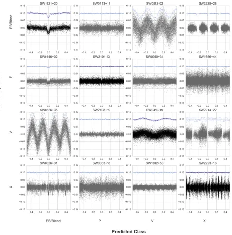
Figure 8. Confusion matrix of RFC results showing examples of light curves selected from samples that fall into each category, chosen to represent typical failure modes. Light curves along the diagonal, shown in black, were correctly classified by the RFC. Off diagonal boxes, shown in grey, were incorrectly identified, with the true classification shown on the vertical axis and the predicted classification shown on the horizontal axis. Looking at the samples in the off-diagonal boxes provide insight into how the RFC makes its decisions and what the common failure modes are. SW1832+53 was labelled as an X in the archive, but the RF predicted it was a variable object. This classification was made early in WASPs’ history, and a clearer picture of the light curve has since been established. While an X classification means that there is no planetary signal, a better classification for the object would be to label it as a variable light curve, which is what the random forest does. SW0826+35 is another interesting object. It was labelled as a variable in the archive, but the alternating depths of dips indicates it may actually be an eclipsing binary, consistent with the machine classification. The final object of special note is SW0146+02, verified as WASP-76b. This planet’s transit is particularly deep and confused the RFC into mislabelling it as an EB/Blend showing that this algorithm is sensitive to the depth of transit despite the classical ‘U’ shape of the event.

of the objects flagged as planets were true positives. It may seem like the CNN would be the best option to use alone, but it did miss several planets that the RFC was able to recover and occasionally let in false signals that were caught by the RFC or SVC, highlighting the importance of combined methods.

We note that the true follow-up rate for any of these methods would be lower in practice. Eclipsing binaries with low-mass stel-lar companions, which closely resemble planets in their light curves and derived features, were removed from the training data set. When we applied the RFC to 399 EBLM systems, 92 (23 per cent) were

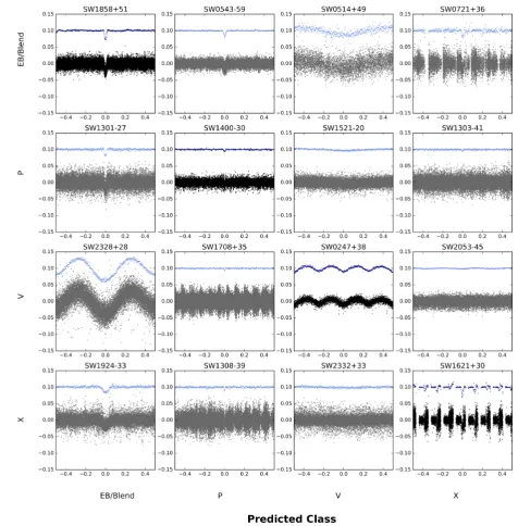
Figure 9. Same as for Fig.8, but for the CNN using the local and full binned light curve. As in the RFC, the overlap in categories in the human classifications is evident in the CNN results. For example, SW1924−33 was labelled by a WASP team member as an X because it does not contain a planetary transit, but it clearly does show a transit event and therefore could be instead classified as an eclipsing binary. While this is considered a wrong classification in the algorithm evaluation, in practice it is an acceptable output. SW1308−39 is an example where near-integer day (in this case near 11 d effects can look like transit signals when the data is phase binned. The CNN did miss several true planets, such as SW1303−41 (WASP-174b; Temple et al.2018), as the dip is very small with a messy light curve. SW1521−20 is an example of a planet found in a different survey (EPIC 249622103; David et al.2018) with the signal not being visible in the WASP data.

classified as planets. The CNN with only the full light curve also returned 64 as planets, partially overlapping with the RFC pre-dictions. Adding the local light-curve information made the CNN more likely to identify EBLMs as planets with 95 (24 per cent) being labelled as planets. The SVC is the most shrewd, with only 24 stars labelled as planets. For many of these objects, the transit signals look identical to those of planets and are only discovered with follow-up information. Even by combining results from

dif-ferent machine-learning methods, we expect to have many of these type of objects flagged for further observation, reducing the overall performance of the algorithms.

There are several caveats to our study. One note of caution is the underlying training data set. The training data was obtained by combining the entries of a number of WASP team members over the course of many years. This leads to two main problems. First, different team members may label the same light curve differently

based on their interpretation. Blends and binaries for example can be used differently by different users. We attempted to control for this by manually inspecting the blends and binaries and updating flags to maintain consistency across all fields. The ‘X’ category is also notably inconsistent, with objects that were rejected as planets for many different reasons, including blends and binaries, being given the same label.

The second issue comes from the fact that the classification be-gan before all current data were available. After the first few WASP observing seasons, classifications were made based on the limited data available. When other data were added in the following seasons, the shape of the light curve may have changed and more (or less) transit-like shapes became obvious. However, since the candidate was already rejected, it was never re-visited and updated. Several examples like this were found by looking through the incorrect

clas-sifications, such as those in Figs8and9, and remained uncorrected

in our training data. Regardless of these problems, the algorithms were robust and were able to make reasonable predictions even with small variations in the training.

Finally, we rely on the BLS algorithm to provide an accurate best-fitting period. This is especially important for the CNN, which only has the light curve folded on that period as input. The CNN is therefore not equipped to handle possible incorrect periods due to aliases or harmonics. It would be possible to augment the code to also include other information for the CNN, such as the data folded on half of the period and twice the period, either in a stack or as a separate entry, to try to identify planets in the data that were found at the wrong period. This possibility will be included in future work, but is beyond the exploratory scope of this paper.

The classifications shown here have a lower accuracy than those

reported in theKeplerstudies, which range from around 87 per cent

up to almost 98 per cent. This is to be expected, as WASP data is unevenly sampled and has much larger magnitude uncertainties, making definitive identifications impossible with WASP data alone. WASP’s large photometric aperture (48 arcsec) also makes con-vincing blends more common. Nevertheless, the machine-learning

algorithms were able to correctly identify∼90 per cent of planets in

the testing data set and operate much faster than human observers (less than 1 min to train the RFC and around 20 min to train the CNNs, and less than a minute to apply to new data sets on a Mac-Book Pro with 3.1 GHz Intel Core i5) and produce more consistent results. The advantage of this is that as new data are added after observing seasons, it is not necessary to look at each light curve again. Rather, the entire data set can be quickly re-run through the algorithms to obtain new observing targets.

In practice, the machine-learning results will be used in combi-nation with expert opinion in order to select the most scientifically compelling targets for follow-up. For example, the area surround-ing the star might be crowded with other stars maksurround-ing follow-up observations difficult. In several cases, a light curve looks promis-ing, but another star within WASP’s pixel resolution has already been labelled as a Blend (often through follow-up) and the label did not propagate to the surrounding light curves. These are easy to identify manually, but that information is not included for the machine-learning algorithms. Therefore, it is still essential that tar-gets selected with machine learning are curated by a human user for practical observation. Another factor only taken partially into account by the RFC is the recent improvement in the knowledge of stellar parallaxes, and hence radius estimates, made possible by the

first and second data releases of theGaiamission (Gaia

Collabora-tion2016,2018). Knowledge of the stellar radius, and therefore the

radius of the transiting object, allows clean dwarf/giant

discrimina-tion, and eliminates an entire subclass of blended eclipsing binaries at a single stroke.

6 C O N C L U S I O N S

While the WASP data alone is not of sufficient quality to definitively identify planets from the data, it has proven to be very effective in producing new candidates for future follow-up and eventual planet status. The large size of the WASP archive makes it undesirable for human observers to manually look at each one to determine whether it is a good candidate for further study. The machine-learning framework we have created provides a tool for the observer wanting to re-examine the full set of data holdings in any WASP field, enabling fast re-classification of all targets showing transit-like behaviour and identification of new targets of interest. This list is not intended to be used as a final list for observing, but rather as a tool for the observers to reduce the total number of light curves requiring analysis. An additional advantage of this approach is that the algorithms can be quickly re-trained as new information, such as new known classifications from completed follow-up observations, become available.

Using multiple machine-learning models is an effective frame-work that can be modified and applied to a variety of different large-scale surveys in order to reduce the total time spent in the target identification and ranking stage of exoplanet discovery. Combining the results from additional machine-learning methods could further improve the predictions.

With the launch of the Transiting Exoplanet Survey Satellite

(TESS; Ricker et al.2014) and upcoming launch of the PLAnetary

Transits and Oscillations of stars (PLATO; Rauer et al.2014),

auto-matic data processing is becoming even more essential. TheTESS

mission will focus on over 200 000 stars with high cadence (∼2 min)

and several million targets with a longer cadence (∼30 min). The

PLATO mission will study an additional million targets. The num-ber of light curves in these data sets is clearly beyond manual classification, so machine-learning techniques will be essential to their success. The application and performance analysis of ma-chine learning on current sky surveys such as WASP are integral to the successful understanding and implementation on future large surveys.

AC K N OW L E D G E M E N T S

NS acknowledges the support of NPRP grant #X-019-1-006 from the Qatar National Research Fund (a member of Qatar Founda-tion). ACC acknowledges support from STFC consolidated grant ST/R000824/1 and UK Space Agency grant ST/R003203/1. DA, FF, DLP, RW, and PJW acknowledge support from STFC through consolidated grants ST/L000733/1 and ST/P000495/1. DJAB ac-knowledges support from the UK Space Agency. FF acknowl-edges support from PLATO ASI-INAF contract no. 2015-019-R0. LM acknowledges support from the Italian Minister of In-struction, University and Research (MIUR) through FFABR 2017 fund. LM also acknowledges support from the University of Rome Tor Vergata through the ‘Mission: Sustainability 2016” fund. DJA gratefully acknowledges support from the STFC via an Ernest Rutherford Fellowship (ST/R00384X/1). SCCB ac-knowledges support by FEDER – Fundo Europeu de Desenvolvi-mento Regional funds through the COMPETE 2020 – Programa Operacional Competitividade e Internacionalizac¸˜ao (POCI), and by Portuguese funds through FCT – Fundac¸˜ao para a Ciˆencia

e a Tecnologia in the framework of the projects POCI-01-0145-FEDER-028953 and POCI-01-0145-FEDER-032113. SCCB also acknowledges the support from FCT and FEDER through COMPETE2020 to grants UID/FIS/04434/2013 & 0145-FEDER-007672, PTDC/FIS-AST/1526/2014 & 01-0145-FEDER-016886, and PTDC/FIS-AST/7073/2014 & POCI-01-0145-FEDER-016880 and through Investigador FCT contract IF/01312/2014/CP1215/CT0004.

We acknowledge Prof Coel Hellier for providing detailed in-formation on the methodology for Southern hemisphere candidate disposition in the later years of the WASP project.

R E F E R E N C E S

Alsubai K. A. et al., 2013, Acta Astron., 63, 465

Armstrong D. J., Pollacco D., Santerne A., 2017,MNRAS, 465, 2634 Armstrong D. J. et al., 2018,MNRAS, 478, 4225

Auvergne M. et al., 2009,A&A, 506, 411 Bakos G. ´A. et al., 2013,PASP, 125, 154 Bentley S., 2009, PhD thesis, Keele Univ. Borucki W. J. et al., 2010,Science, 327, 977 Breiman L., 2001,Mach. Learn., 45, 5 Brown T. M., 2003,ApJ, 593, L125

Cameron A. C., Jardine M., 2018, MNRAS, 476, 2542 Carrasco D. et al., 2015,A&A, 584, A44

Chawla N. V., Bowyer K. W., Hall L. O., Kegelmeyer W. P., 2002, J. Artif. Int. Res., 16, 321

Chollet F. et al., 2015, Keras, https://github.com/fchollet/keras

Christian D. J. et al., 2006,MNRAS, 372, 1117 Collier Cameron A. et al., 2006,MNRAS, 373, 799 Collier Cameron A. et al., 2007,MNRAS, 380, 1230 Cortes C., Vapnik V., 1995,Mach. Learn., 20, 273 Cover T., Hart P., 1967,IEEE Trans. Inf. Theor., 13, 21

D’Isanto A., Cavuoti S., Brescia M., Donalek C., Longo G., Riccio G., Djorgovski S. G., 2016,MNRAS, 457, 3119

David T. J. et al., 2018,AJ, 155, 222

Dittmann J., Irwin J., Charbonneau D., Bonfils X., Astudillo N., Newton E. R., Berta-Thompson Z. K., 2017, American Astronomical Society Meeting Abstracts #229, p. 415.01

du Buisson L., Sivanandam N., Bassett B. A., Smith M., 2015,MNRAS, 454, 2026

Dubath P. et al., 2011,MNRAS, 414, 2602 Gaia Collaboration, 2016,A&A, 595, A1 Gaia Collaboration, 2018, A&A, 616, A1, Gaidos E. et al., 2014,MNRAS, 437, 3133

Gray D. F., 1992, The Observation and Analysis of Stellar Photospheres. Cambridge University Press, Cambridge, UK

Hartman J. D., Bakos G., Stanek K. Z., Noyes R. W., 2004,AJ, 128, 1761 He K., Zhang X., Ren S., Sun J., 2016, Deep Residual Learning for Image

Recognition, 2016 IEEE Conference on Computer Vision and Pattern Recognition (CVPR)

Hon M., Stello D., Yu J., 2017,MNRAS, 469, 4578

Huppenkothen D., Heil L. M., Hogg D. W., Mueller A., 2017,MNRAS, 466, 2364

Kingma D. P., Ba J., 2014, preprint (arXiv:1412.6980) Kipping D. M., Lam C., 2017,MNRAS, 465, 3495 Kov´acs G., Zucker S., Mazeh T., 2002,A&A, 391, 369 Kov´acs G., Bakos G., Noyes R. W., 2005,MNRAS, 356, 557 Kreidberg L., 2015,PASP, 127, 1161

Krizhevsky A., Sutskever I., Hinton G. E., 2012, in Pereira F., Burges C.J.C., Bottou L., Weinberger K.Q., eds, Advances in Neural Information Pro-cessing Systems 25. Curran Associates, Inc., p. 1097

LeCun Y., Boser B. E., Denker J. S., Henderson D., Howard R. E., Hub-bard W. E., Jackel L. D., 1990, ImageNet Classification with Deep Convolutional Neural Networks. in Touretzky D. S., ed., Advances in Neural Information Processing Systems 2. Morgan-Kaufmann, p.

396,http://papers.nips.cc/paper/293-handwritten-digit-recognition-wit h-a-back-propagation-network.pdf

LeCun Y., Bottou L., Orr G. B., M¨uller K. R., 1998, Efficient BackProp. Springer, Berlin, Heidelberg, p. 9,https://doi.org/10.1007/3-540-4943 0-8 2

Lecun Y., Bengio Y., Hinton G., 2015,Nature, 521, 436

Lo K. K., Farrell S., Murphy T., Gaensler B. M., 2014,ApJ, 786, 20 Masci F. J., Hoffman D. I., Grillmair C. J., Cutri R. M., 2014,AJ, 148, 21 McCauliff S. D. et al., 2015,ApJ, 806, 6

Mislis D., Bachelet E., Alsubai K. A., Bramich D. M., Parley N., 2016,

MNRAS, 455, 626

Morii M. et al., 2016,PASJ, 68, 6

Nair V., Hinton G. E., 2010, in Proceedings of the 27th International Con-ference on Machine Learning. ICML’10. p. 807

Naul B., Bloom J., P´erez F., van der Walt S., 2017,Nat. Astron., 2, 151 Pashchenko I. N., Sokolovsky K. V., Gavras P., 2018,MNRAS, 475, 2326 Pearson K. A., Palafox L., Griffith C. A., 2018,MNRAS, 474, 478 Pedregosa F. et al., 2011, J. Mach. Learn. Res., 12, 2825 Pepper J. et al., 2007,PASP, 119, 923

Perruchot S. et al., 2011, in Proc SPIE Conf. Ser. Vol. 8151, Techniques and Instrumentation for Detection of Exoplanets V. SPIE, Bellingham, p. 815115

Pollacco D. L. et al., 2006,PASP, 118, 1407 Queloz D. et al., 2000, A&A, 354, 99 Rauer H. et al., 2014,Exp. Astron., 38, 249

Ricker G. R. et al., 2014, in Proc. SPIE Conf. Ser. Vol. 9143, Space Telescopes and Instrumentation 2014: Optical, Infrared, and Millimeter Wave. SPIE, Bellingham, p. 914320

Rimoldini L. et al., 2012,MNRAS, 427, 2917 Shallue C. J., Vanderburg A., 2018,AJ, 155, 94

Tamuz O., Mazeh T., Zucker S., 2005,MNRAS, 356, 1466 Temple L. Y. et al., 2018, MNRAS, 480, 5307

Yu H.-F., Huang F.-L., Lin C.-J., 2011,Mach. Learn., 85, 41 Zhu W. W. et al., 2014,ApJ, 781, 117

S U P P O RT I N G I N F O R M AT I O N

Supplementary data are available atMNRASonline.

Appendix 1. Confusion matrices for the Linear Support Vector, Support Vector, Logistic Regression, K-nearest neighbours, and Random Forest classifiers. The confusion matrices reflect the per-formance of the classifiers on the testing data set, made up of 2314 total light curves. The left column shows the results of the classi-fiers when trained only on the 4697 real data points in the training data set. The right column shows the performance of the classifiers when the training data set also includes additional synthetic data points created with SMOTE resampling. In all cases, the test data set remains the same.

Please note: Oxford University Press is not responsible for the content or functionality of any supporting materials supplied by the authors. Any queries (other than missing material) should be directed to the corresponding author for the article.

1_{Centre for Exoplanet Science, SUPA, School of Physics and Astronomy,}

University of St Andrews, St Andrews KY16 9SS, UK

2_{Institut d’astrophysique de Paris, UMR7095 CNRS, Universit´e Pierre &}

Marie Curie, 98bis boulevard Arago, F-75014 Paris, France

3_{Observatoire de Gen`eve, Universit´e de Gen`eve, 51 Chemin des Maillettes,}

CH-1290 Sauverny, Switzerland

4_{School of Physics & Astronomy, University of Birmingham, Edgbaston,}

Birmingham B15 2TT, UK

5_{Universit´e Grenoble Alpes, CNRS, IPAG, F-38000 Grenoble, France}

6_{Qatar Environment and Energy Research Institute (QEERI), Hamad Bin}

Khalifa University (HBKU), Qatar Foundation, Doha, Qatar

7_{Astrophysics Group, Keele University, Staffordshire ST5 5BG, UK}

8_{Centre for Exoplanets and Habitability, University of Warwick, Gibbet Hill}

Road, Coventry CV4 7AL, UK

9_{Department of Physics, University of Warwick, Coventry CV4 7AL, UK}

10_{Instituto de Astrof´ısica e Ciˆencias do Espac¸o, Universidade do Porto,}

CAUP, Rua das Estrelas, P-4150-762 Porto, Portugal

11_{Institute for Astronomy, Astrophysics, Space Applications and Remote}

Sensing, National Observatory of Athens, 15236 Penteli, Greece

12_{INAF – Osservatorio Astrofisico di Catania, Via S. Sofia 78, I-95123}

Catania, Italy

13_{Department of Physics, Hobart and William Smith Colleges, Geneva, NY}

14456, USA

14_{Department of Physics, University of Rome Tor Vergata, Via della Ricerca}

Scientifica 1, I-00133 Roma, Italy

15_{Max Planck Institute for Astronomy, K¨onigstuhl 17, D-69117 Heidelberg,}

Germany

16_{INAF – Astrophysical Observatory of Turin, Via Osservatorio 20, I-10025}

Pino Torinese, Italy

17_{International Institute for Advanced Scientific Studies (IIASS), Via G.}

Pellegrino 19, I-84019 Vietri sul Mare (SA), Italy

18_{Instituto de Astrosf´ısica de Canarias (IAC), E-38205 La Laguna, Tenerife,}

Spain

19_{Departamento de Astrof´ısica, Universidad de La Laguna (ULL), E-38206}

La Laguna, Tenerife, Spain

20_{Cavendish Laboratory, JJ Thompson Avenue, Cambridge CB3 0HE, UK}

This paper has been typeset from a TEX/LA_{TEX file prepared by the author.}