Tracking marine mammals in 3D using electronic tag
1data
2Christophe Laplanchea,b, Tiago A. Marquesc, Len Thomasc 3
aUniversit´e de Toulouse; INP, UPS; EcoLab (Laboratoire Ecologie Fonctionnelle et 4
Environnement); ENSAT, Avenue de l’Agrobiopole, 31326 Castanet Tolosan, France
5
bCNRS; ECOLAB; 31326 Castanet Tolosan, France
6
c Centre for Research into Ecological and Environmental Modelling, The Observatory, 7
Buchanan Gardens, University of St Andrews St Andrews, KY16 9LZ, Scotland, UK
8
Abstract
9
running title: 3D marine mammal tracking
10
word count (including tables, figure captions and references): 7858
11
1. Information about at depth behaviour of marine mammals is funda-12
mental yet very hard to obtain from direct visual observation. Animal 13
borne multi-sensor electronic tags provide a unique window of observa-14
tion into such behaviours. 15
2. Electronic tag sensors allow the estimation of the animal’s 3-dimensional 16
(3D) orientation, depth, and speed. Using tag flow noise level to pro-17
vide an estimate of animal speed we extend existing approaches of 3D 18
track reconstruction by allowing the direction of movement to differ 19
from that of the animal’s longitudinal axis. 20
3. Data are processed by a hierarchical Bayesian model that allows pro-21
cessing of multi-source data, accounting for measurement errors, and 22
testing hypotheses about animal movement by comparing models. 23
4. We illustrate the approach by reconstructing the 3D track of a 52-24
minute deep dive of a Blainville’s beaked whaleMesoplodon densirostris 25
adult male fit with a digital tag (DTAG) in the Bahamas. At depth, 26
the whale alternated regular movements at large speed (>1.5 m/s) and 27
more complex movements at lower speed (<1.5 m/s) with differences 28
between movement and longitudinal axis directions of up to 28◦. The 29
reconstructed 3D track agrees closely with independent acoustic-based 30
5. The approach is potentially applicable to study the underwater be-32
haviour (e.g. response to anthropogenic disturbances) of a wide variety 33
of species of marine mammals fitted with triaxial magnetometer and 34
accelerometer tags. 35
Keywords: dead reckoning, animal movement modelling, electronic tag, 36
hierarchical Bayesian modelling, track reconstruction, triaxial 37
magnetometer and accelerometer, flow noise 38
1. Introduction
39
The use of animal borne autonomous recording tags to collect information 40
for inferences on movement, ecology, physiology and behaviour is becoming 41
widespread, providing an unprecedented window into these biological pro-42
cesses and leading to otherwise unattainable discoveries, especially at sea 43
where animal behaviour is hard to observe directly (Ropert-Coudert & Wil-44
son, 2005; Bograd et al., 2010). 45
Initially used simply to identify animals, over time tags became equipped 46
with thermometers and barometers, followed by accelerometers, magnetome-47
ters, gyroscopes, microphones, hydrophones, GPSs, and even video (e.g. 48
Johnson et al., 2009; Burgess, 2009; Marshall et al., 2007; Rutz & Tros-49
cianko, 2013). Some tags provide direct information on location while others 50
do not. For those that do, say via GPS or radio tracking, a common approach 51
has been to use state space models or hidden Markov models to reconstruct 52
two dimensional tracks (e.g. Jonsen et al., 2012; Beyeret al., 2013; Langrock 53
et al., 2014). However, most marine mammals spend a large proportion of 54
their time at depth, hence accounting for the depth component might be 55
fundamental, depending on each study’s objectives (e.g. Tracey et al., 2014). 56
Published tracks in 3 dimensions (3D) are based on some form of dead 57
reckoning (Wilson et al., 2007): each position is predicted by updating the 58
previous time step position considering an estimate of the animal’s current 59
direction and speed. One option is to infer animal 3D speed from 3D orien-60
tation (computed from accelerometer and magnetometer data) and vertical 61
speed (from depthmeter data). However, this is sensitive to error in depth 62
measurements, notably when animal movement is close to horizontal. This 63
has led to estimating speed from other sources than depthmeters, namely 64
have required the assumption that the direction of animal movement coin-66
cides with the direction of its longitudinal (rostro-caudal for a whale) axis, 67
i.e. the animal moves towards where it is pointing. If this does not hold, bias 68
can be expected, and the resulting track will be unreliable (Johnson et al., 69
2009). Further, errors accumulate over time, a phenomena referred to as drift 70
(Wilson et al., 2007). Additional drifting due to external factors can occur 71
(e.g. Shiomi et al., 2008). Therefore, while tags are very useful to establish 72
relative positions of animals, inferring absolute position is questionable with 73
existing procedures: the term pseudo-track is used to reinforce the notion 74
that absolute position is unknown (Hazen et al., 2009). Also for this reason, 75
dead-reckoning tracks are often “anchored” to known positions (e.g. Zimmer 76
et al., 2005; Hazen et al., 2009; Friedlaender et al., 2009). These are some-77
times referred to as geo-referenced tracks, to convey the notion of absolute 78
position on the earth sphere. However, measurement error in positions is typ-79
ically ignored, and the way the pseudo-track is combined with these is not 80
explicitly described (e.g. Davis et al., 2001; Mitani et al., 2003; Tysonet al., 81
2012). Nonetheless, implementation details can have considerable impact on 82
the estimated track, as well as (if estimated) on its precision. 83
We consider DTAGs (Johnson & Tyack, 2003) as an example. DTAGs 84
include triaxial accelerometer and magnetometer sensors, a pressure sensor 85
(sampling rate up to 50 Hz), and two hydrophones (up to 192 kHz) (Johnson 86
& Tyack, 2003). Other tags (e.g. “OpenTag”, Loggerhead Instruments, Sara-87
sota, FL, USA) include triaxial magnetometers and accelerometers. Around 88
20 marine mammal species (>1000 deployments) including whales, dolphins 89
and pinnipeds have been fitted with DTAGs (Mark Johnson, pers. comm.). 90
Such tags have become widespread in marine mammal studies, allowing in-91
ferences about at depth behaviour and ecophysiology (e.g. Watwood et al., 92
2006; Shaffer et al., 2013). DTAGs were originally developed to infer be-93
haviour and relative movement rather than absolute location, having been 94
used extensively for this purpose – e.g., recent work on feeding behaviour 95
in baleen whales (e.g. Simon et al., 2012; Ware et al., 2014, and references 96
therein). However, DTAG data have been used to reconstruct 3D dives of 97
animals (e.g. Davis et al., 2001; Mitani et al., 2003; Johnson & Tyack, 2003; 98
Madsen et al., 2005). Bespoke software is now available to process tag data 99
into tracks (the R packages animalTrack, Farrell & Fuiman (2014), and 100
TrackReconstruction, Battaile (2014), and to depict 3D tracksTrackplot, 101
Wareet al. (2006)). An estimated position without an associated measure of 102
mate. Nonetheless existing software does not provide uncertainty on position 104
estimates, so these are never reported. 105
Extending dead reckoning and georeferencing methods described earlier, 106
we develop a new way to use magnetometer and accelerometer tag data to 107
reconstruct 3D tracks and estimate associated uncertainty. We explicitly (1) 108
incorporate measurement error, both from the tag and from estimated posi-109
tions, in the input data and propagate this error through to the estimated 110
track; (2) include information about animal speed both from change in depth 111
given orientation and from tag flow noise; and (3) utilize the additional in-112
formation from both sources of speed information to relax the assumption 113
that the animal moves in the direction it is pointed. Our model is superfi-114
cially similar to well-known 2D random walk models by, e.g., Jonsen et al. 115
(2005), Moraleset al. (2004) and McClintocket al. (2012) in that, like them, 116
we model animal speed (i.e. step length) and movement direction in dis-117
crete time and continuous space, and use Bayesian methods to link models 118
to data. However, assumptions about animal movement differ. Random walk 119
models make distributional assumptions about step length and direction (or 120
turning angle), hence resulting track estimates are a combination of the as-121
sumed movement model and the input data (filtered through the observation 122
process); by contrast we do not make such assumptions, hence our estimated 123
tracks are a function of the data and observation process alone. In this sense, 124
our approach is more “data focused”, but is also more reliant on having high 125
frequency, high quality data to produce a realistic track. We return to these 126
issues in the Discussion. 127
We illustrate our method by reconstructing a 52-minute dive of a tagged 128
Blainville’s beaked whale Mesoplodon densirostris (Laplanche et al., 2015), 129
for which independent underwater localizations are available. These are not 130
used in model fitting; instead we use them to evaluate the accuracy of the 131
estimated track derived from tag data alone. Finally, we discuss the capabil-132
ities of the approach and possible improvements. 133
2. Materials and methods
134
2.1. Tag measurements and coordinate systems 135
We consider three coordinate systems (or frames) to accurately describe 136
animal movement and tag data: (1) the Earth frame, a cartographic pro-137
jected coordinate system (x-axis south-north, positive north; y-axis east-138
location at the sea surface), (2) the animal frame (x-axis, longitudinal axis, 140
positive forward; y-axis, right-left axis, positive left; z-axis, dorso-ventral 141
axis, positive up; origin is the geometric center of the animal), and (3) the 142
tag frame (x-,y-,z-axes are internally defined; origin is the center of the tag) 143
– this latter frame is required because the tag is not always placed with the 144
same orientation on the animal. 145
An animal’s 3D track is the time-series of its 3D location; more specifically 146
the 3D Cartesian coordinates of the origin of the animal frame in the Earth 147
frame, denoted x(t) = (x(t), y(t), z(t)) at time t. Animal 3D speed is the 148
time derivative of x(t); the speed of translation of the animal frame in the 149
Earth frame, denoted v(t) = (vx(t), vy(t), vz(t)). The orientation of a 3D 150
object in space is unambiguously described in terms of heading h (rotation 151
to the z-axis, h∈ (−180◦,180◦]), pitch p(y-axis, p∈ (−90◦,90◦]), and roll 152
r (x-axis, r ∈ (−180◦,180◦]) with respect to some frame of reference. The 153
animal’s 3D orientation at time tis represented by its heading h(t) (positive 154
Eastwards), pitch p(t) (positive upwards) and roll r(t) (positive rightwards), 155
with respect to the Earth frame. 156
Tag data are not directly available in the Earth frame. Accelerometer 157
and magnetometer measure the Earth’s gravitationnal and magnetic fields 158
in the tag frame. The conversion of Earth’s gravitationnal and magnetic fields 159
between animal and Earth frames is achievedvia rotation matrices described 160
in the next section. The conversion of raw accelerometer and magnetometer 161
data in the tag frame into the animal frame is achieved in a similar way. 162
Description of the latter process, together with the processing of acoustic 163
data into flow noise level, is deferred to Section 2.5. 164
2.2. The statistical model 165
We describe the full statistical model here. Approximations used in prac-166
tice for computational efficiency are described in Section 2.3. 167
The objective is to use available tag data (Earth’s gravitationnal and 168
magnetic fields in the animal frame, depth, flow noise level), and independent 169
positional data, if available, to infer unknown, latent variables characterizing 170
animal movement (x(t), v(t), h(t), p(t), and r(t)). Our implementation 171
utilizes a hierarchical Bayesian model (HBM). The overall model structure 172
is illustrated in Figure 1, relating latent and measured variables as detailed 173
below. For clarity the model is presented in four sections: (1) estimation 174
of animal orientation from accelerometer, magnetometer and depth-meter 175
direction of movement from a combination of speed, orientation and change in 177
depth; (3) track estimation, and (4) incorporation of independent positional 178
information. 179
We define t0 and tend as the track start and end times, t∈[t0, tend]. 180
2.2.1. Animal 3D orientation 181
The expected values Aa(t) and Ma(t) of the 3D Earth gravitationnal 182
and magnetic fields in the animal frame (superscript a) at time t are 183
Aa(t) =T(t)Ae
Ma(t) =T(t)Me, (1)
where T(t) is a rotation matrix that switches from the Earth frame to the 184
animal frame given by 185
T(t) =
1 0 0
0 cosr(t) sinr(t)
0 −sinr(t) cosr(t)
×
cosp(t) 0 sinp(t)
0 1 0
−sinp(t) 0 cosp(t)
×
cosh(t) sinh(t) 0
−sinh(t) cosh(t) 0
0 0 1
,
(2)
and Ae and Me are the values of the 3D Earth gravitational and magnetic 186
fields in the Earth frame (superscript e) at the tagging location and time. 187
Given the relative small scale of most studies, ours included, compared to 188
these 3D Earth fields, these can safely be treated as constants. They can 189
be either measured or derived from models of the gravitational and Earth 190
magnetic fields. 191
Measured (superscriptobs) values of the Earth gravitational (Aa,obs(t)= 192
and magnetic fields (Ma,obs(t)) in the animal frame at timet are modelled 193
as multivariate Gaussian distributions (MVN) 194
Aa,obs(t)∼MVN(Aa(t),Σ A(t)) Ma,obs(t)∼MVN(Ma(t),Σ
M(t))
(3)
where ΣA(t) and ΣM(t) are time-dependent covariance matrices (see Ap-195
pendix S1 for details). The observed animal depth is 196
where z(t) is the unobserved true depth of the animal in the Earth frame 197
and σz2 is the depth-meter measurement error variance. 198
2.2.2. Animal speed and direction of movement 199
We explicitly relax what we refer in the following as the equal pitch as-200
sumption: that the direction of animal movement coincides with the direction 201
of its longitudinal axis. Animal speed animal at time t is 202
vx(t) = cosh0(t) cosp0(t)v(t) vy(t) = −sinh0(t) cosp0(t)v(t) vz(t) = sinp0(t)v(t),
(5)
where v(t) = ||v(t)||, h0(t), and p0(t) are the Euclidean norm, the heading 203
(positive Eastwards), and the pitch (positive upwards) in the Earth frame of 204
the speed vector of the animal at time t. Differences of orientations of the 205
longitudinal axis and the speed vector are modeled as differences in respective 206
pitch angles 207
p0(t)∼Normal(p(t), σp2), p0(t)∈(−90,90], (6)
where σ2
p is the variance of the pitch difference ∆p(t) = p(t)− p
0(t). We
208
refer in the following to this as the unequal pitch assumption and to ∆p(t) as 209
pitch anomaly. A positive pitch anomaly occurs when the animal points its 210
longitudinal axis higher than expected by its swimming direction, and vice 211
versa (Figure 2). Pitch anomaly can be the result of a pitch and/or a heading 212
movement in the animal frame depending on the roll. For reasons discussed 213
later, we do not consider heading anomaly, hence assuming h(t) =h0(t). 214
Animal speed is related to background noise level NL(t) at time t assum-215
ing 216
v(t)∼Normal(av+bvlog(NL(t)), σ2v), v(t)≥0, (7)
where av and bv are regression parameters and σv is the residual standard 217
error (Appendix S2). 218
2.2.3. Animal 3D track 219
Animal Cartesian coordinates at time t+ ∆t are computed from coordi-220
nates at time t and speed: 221
x(t+ ∆t) =x(t) +vx(t)∆t y(t+ ∆t) = y(t) +vy(t)∆t z(t+ ∆t) =z(t) +vz(t)∆t
2.2.4. Independent positional information 222
In our application we only use information about the dive starting po-223
sition, assumed to have been observed with known error. We model this 224
as 225
xobs(t
0)∼Normal(x(t0), σ2x(t0)) yobs(t
0)∼Normal(y(t0), σy2(t0))
(9)
where σ2
x(t0) and σ2y(t0) are known variance terms. If the absolute start 226
position is unknown, arbitrary values are provided for (xobs(t
0), yobs(t0)) with 227
null variances (σx2(t0) = σ2y(t0) = 0); estimated locations become relative to 228
this position. 229
Similarly, additional animal positions might be used to improve the track 230
reconstruction process. When at the surface these could come from visual 231
observations, animal-borne GPS or satellite receivers. When underwater, 232
these could come from passive (or active) acoustic localizations. 233
2.2.5. Priors 234
Prior distributions are required on all top-level random variables in the 235
hierarchical model. Observation variance parameters are assumed known, 236
hence not requiring priors. We also assume the relationship between mea-237
sured noise level and speed is known with certainty (see Section 2.3 and 238
Discussion). These variables are shown as grey boxes in Figure 1. The re-239
maining top-level variables are pitch, heading and roll at each time step, for 240
which uniform distributions are assumed: 241
p(t)∼Uniform(−90,90) h(t)∼Uniform(−180,180) r(t)∼Uniform(−180,180)
(10)
2.3. Bayesian computation and approximating model 242
The model described by equations (1)-(10) is not analytically tractable; 243
however, samples from the posterior distribution of latent variables can be 244
simulated via Markov chain Monte Carlo (MCMC). For this, we used Open-245
BUGS version 3.2.1, open-source version of WinBUGS (Ntzoufras, 2009). 246
BUGS code is available as Appendix S3. Tag data preprocessing and output 247
postprocessing were implemented in R (R Core Team, 2013). 248
Initial runs showed that the full model was highly computer-intensive. 249
Two procedures were implemented to reduce computing time, both of which 250
divided into three stages (and each stage was analyzed in turn): (i) compute 252
animal 3D orientation (equations 1 - 4, 10); (ii) calibrate the speed-noise 253
relationship (equation 7); (iii) compute animal 3D track (equations 5, 6, 8, 254
9). Uncertainty was propagated across stages by modelling stage outputs 255
as Gaussians, with mean and variance equal to the corresponding posterior 256
values, using this distribution as input to the next stage. However, in moving 257
from stage (ii) to (iii) the parameters of the speed-noise model were assumed 258
known. Secondly, in computing stages (i) and (iii), the track was divided into 259
1-minute pieces. Each piece was run in parallel using a high performance 260
computing resource (HPR). Pieces were then joined and uncertainty from 261
the end of each piece propagated to the beginning of the next (see Appendix 262
S4 for details and discussion for possible impacts). 263
MCMC convergence was assessed by computing the inter-chain variances 264
of the simulated latent variable samples across 4 chains. For each chain, once 265
convergence was reached, 10,000 samples were simulated; these were thinned 266
to 1,000 independent samples per chain, with thinning guided by analyzing 267
the autocorrelation function of the posterior samples. Reported point esti-268
mates are posterior means, standard errors are posterior standard deviations 269
(reported as mean±standard error), and reported interval estimates are 2.5 270
% and 97.5 % posterior marginal quantile estimates. 271
2.4. Alternative models for pitch anomaly 272
The model assumes a fixed pitch anomaly standard deviation σp (see
273
Discussion for a relaxation of this assumption). To investigate how pitch 274
anomaly varied along the track we repeated the above analysis considering 275
three different values for σp: 0◦, 5◦ and 10◦. These represent three different 276
models and we denote them M0, M5 and M10, respectively. 277
Models were compared, for each track piece, using the Deviance Infor-278
mation Criterion (DIC Spiegelhalter et al., 2002), a goodness-of-fit index 279
penalized for model complexity, similar in spirit to Akaike’s Information Cri-280
terion; smaller values are considered better (see Section 4 for a discussion 281
of alternative model selection measures). Following Gelman et al. (2003) we 282
estimated model complexity as pv = var{−2 log[p(θ|y)]}/2. The models do 283
not share the same complexity: M0 is the least complex (p0(t) is perfectly 284
known given p(t)), which is less complex than M5 (p0(t) estimated under 285
the more relaxed constraint of equation (6) with σp = 5◦) which is itself less 286
complex than M10 (even more relaxed constraint with σp = 10◦). In the 287
2.5. Example dataset 289
For illustration we used a Mesoplodon densirostris Blainville’s beaked 290
whale adult male tagged on the 5thSeptember 2007 (tag on position: 24.3839 291
N, 77.5615 W) at AUTEC (Atlantic Undersea Test and Evaluation Center, an 292
instrumented US Navy testing range in the Bahamas). AUTEC details and a 293
different analysis of this DTAG data can be found in Ward et al.(2011). We 294
illustrate the methods using the first deep dive, which lasted 5102000 (full tag 295
deployment: 16 hours, 5 deep dives). Mesoplodon densirostris depth profiles 296
have been modelled using behaviour states (Langrock et al., 2013), and deep 297
dives can be divided in descent, foraging and ascent phases: here the whale 298
fluked up and initiated its dive at arbitrarily fixed t0 = 0, ended its descent 299
and started active searching for prey at tB = 705000, stopped active searching 300
for prey and initiated its ascent at tC = 3503000, and reached the surface at 301
tend= 5102000. 302
The magnetic field was computed by using the IGRF11 (11th
Genera-303
tion International Geomagnetic Reference Field) Earth’s main magnetic field 304
model (International Association of Geomagnetism and Aeronomy, Work-305
ing Group V-MOD, 2010). The magnetic field at the tagging location and 306
time wasMe = (25736,3205,−35522) nT (declination: 7.15◦ W; inclination:
307
54.08◦ down). The gravitational field wasAe = (0,0,−9.79) m/s2. Arbitrary 308
null values were provided for the location of the whale at the beginning of 309
the dive (xobs(t
0) =yobs(t0) = 0 m with σx2(t0) =σy2(t0) = 0 m). 310
Raw tag-frame accelerometer and magnetometer data were converted into 311
animal-frame accelerometer and magnetometer data as described by Johnson 312
& Tyack (2003). Accelerometer, magnetometer, and depth-meter data were 313
lowpass filtered by using a 1-second, squared-window rolling mean before 314
being downsampled at 1 Hz (∆t= 1 s). Background noise level was evaluated 315
as the median of the absolute value of the acoustic samples over a 1-second 316
window before being downsampled at 1 Hz. This simple procedure is robust 317
to the presence of transient signals, in our case echolocation signals emitted 318
by the tagged animal. 319
Eight independent acoustic localizations with low measurement error were 320
available (at 7’40, 10’40, 10’44, 29’21, 29’22, 29’23, 29’24, and 29’33), ob-321
tained by cross referencing data from AUTEC range hydrophones with the 322
known times of emission of clicks from the tag (see Ward et al. (2011) for 323
details). These were ignored in the modelling, providing instead an inde-324
pendent comparison to our location results. For comparison, a conventional 325
with 4 states (x, y, z, speed) and 1 observation (depth). Heading and pitch 327
were treated as known covariates, fitted via a Kalman filter, implemented in 328
R. 329
3. Results
330
The dive track reconstruction (for all 3 models) on a single MCMC 331
chain would have required 65 h of computation time on a single core of a 332
IntelR Xeon E5-2680v2 2.8Ghz 10-core processor. This was reduced to 75 333
minutes using HPR (Appendix S4). 334
Estimates of whale heading, pitch, and roll for the complete dive are 335
provided as Appendix S5. The standard deviations of the whale
head-336
ing, pitch, and roll estimates were 0.78◦ (average for the whole dive, 95 % 337
in (0.35◦,1.31◦)), 0.35◦ (0.18◦,0.54◦), and 0.47◦ (0.14◦,1.01◦), respectively. 338
These quantify observation measurement error in heading, pitch, and roll. 339
Animal speed is linearly predicted from log-transformed flow noise level 340
(R2 = 0.77, Appendix S2). 341
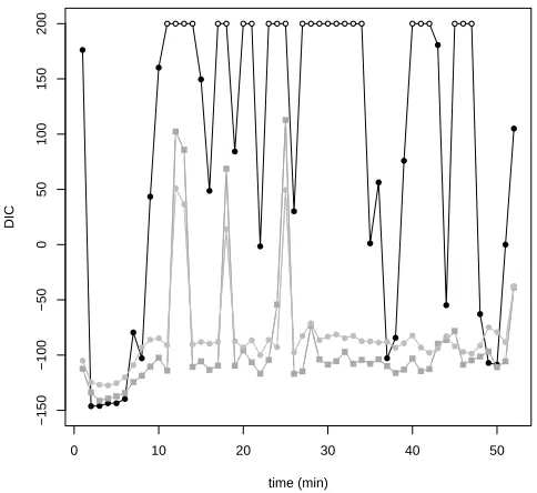
DIC values are shown in Figure 3. ModelM0 was favoured from 10 to 50. 342
ModelM5 performed better for the rest of the dive except for 4 dive portions 343
(at 120, 180, 250, 450) whereM10 was favoured. M0 better performance at the 344
beginning of the dive (similar fit with lower complexity) can be explained by 345
the whale’s negligible pitch anomaly at this stage leading to the equal pitch 346
assumption. The improvement provided by M5 and M10 for the rest of the 347
dive (better fit despite higher complexity) suggests a non negligible pitch 348
anomaly and consequent need for equation (6). ModelM5 performed better 349
than M10 for most of the dive (similar goodness-of-fit with lower complex-350
ity) indicating that the flexibility introduced by setting σp = 5◦ should be 351
preferred to σp = 10◦. Nonetheless, M10 outperformed M5 for some dive 352
portions (better fit despite higher complexity) with higher amplitude pitch 353
anomaly. Overall, results strongly favor the unequal pitch assumption and 354
σp = 5◦. The following results are exclusively based on model M5, but this 355
choice is not critical, as localization results are similar by using σp = 10◦ 356
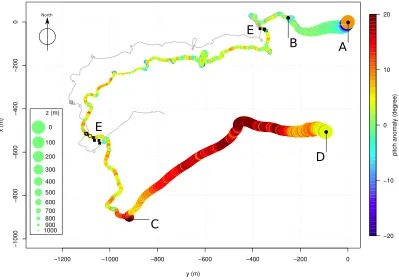
(distance between tracks: 17.4±14.5 m). The whale’s estimated 3D track 357
is illustrated in Figure 4 (interval estimates are provided as Appendix S5). 358
The absolute distance between the results from the independent acoustic 359
survey localizations and the estimated track from M5 is 38.3±18.7 m. For 360
comparison a standard dead-reckoning track fitted using a Kalman Filter is 361
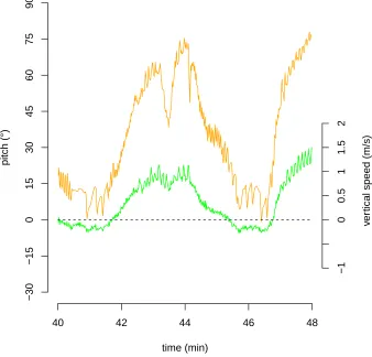
pitch anomaly is illustrated in Figure 5. The whale initiated its dive with a 363
strongly negative pitch anomaly (−20◦), pitch anomaly rapidly reached zero 364
(t ∈ [0000,0040]) and stabilized (peak-to-peak lesser than 4◦, t ∈ [2000,6000] 365
and up to 15◦ fort∈[6000,7050]). At depth (t∈[7050,35030]), the whale alter-366
nated sections with either moderate pitch anomaly variations (peak-to-peak 367
lesser than 10◦) or strong variations (peak-to-peak up to 40◦). During the 368
ascent (t∈ [35030,51020]), the whale had a positive pitch anomaly (between 369
5◦ and up to 28◦). At depth, sections of large speed were associated with 370
moderate pitch anomaly variations and sections of low speed were associated 371
with strong pitch anomaly variations, suggesting that the whale alternated 372
complex rotational movements at low speed and more regular movements 373
at higher speed. During the ascent, the whale always kept a positive pitch 374
while the vertical speed could be negative (as low as−0.40 m/s) as illustrated 375
in Figure S2-2 (Appendix S2). The whale alternated active fluking (strong 376
variations in speed) and passive gliding (no variation) with a strong positive 377
pitch anomaly for the whole ascent. 378
4. Discussion
379
We used a relatively simple “data driven” model, where expected ori-380
entation is a function of accelerometer and magnetometer measurements, 381
expected speed is a function of measured noise and pitch anomaly is a func-382
tion of speed and measured changed in depth. Measurement error on the 383
observed quantities was assumed Gaussian, with known variance (except for 384
variance in the speed vs. flow noise relationship, which was estimated). This 385
approach can be expected to produce a realistic track where high quality 386
(i.e., low error), high frequency data are available that relate closely to ani-387
mal orientation and speed. DTAGs generate exactly such data. By contrast, 388
where the data give less accurate information about animal movement or po-389
sition, and/or are collected much less frequently, then it becomes necessary 390
to include assumptions about the underlying movement behaviour of the an-391
imal in the model – for example using a biased correlated random walk, with 392
model parameters representing centres of attraction or repulsion and corre-393
lation between time steps (e.g. McClintock et al., 2012). A good example of 394
such data is Argos satellite tags (see, e.g. McClintock et al., 2015). One ad-395
vantage of our approach is that the track is not constrained by assumptions 396
about movement behaviour. Disadvantages include it: (1) requires high qual-397
behaviour (except in the specification of different error variances in differ-399
ent diving phases); (3) does not directly allow biological inferences about 400
movement (in contrast with, e.g., the multi-state models of McClintocket al. 401
(2012) – although such inferences could be made in a second analysis stage; 402
(4) cannot be used for simulating tracks, since it relies on input data at each 403
time step. Therefore, the most appropriate approach depends on the data 404
available and the goals of the analysis. 405
Reconstructing 3D tracks from accelerometer, magnetometer, and depth-406
meter data alone, by implicitly assuming that the animal is moving in the 407
direction of its longitudinal axis, might lead to biased inferences (see Figure 408
4). As illustrated in Figure S2-2 (Appendix S2), the whale’s movement direc-409
tion does not necessarily coincide with its longitudinal axis during the ascent. 410
Therefore the animal is capable of having a movement direction different to 411
its own axis, issuing a serious warning against the equal pitch assumption. 412
The inability to estimate speed when the animal is approximately horizontal 413
(Appendix S2) represents an additional argument against reconstructing 3D 414
tracks from accelerometer, magnetometer, and depthmeter data alone. 415
Following previous work (e.g. Simon et al., 2009; Ware et al., 2011) we 416
estimated speed from an independent source, modeling the speed/noise re-417
lationship using the animal’s steep descent phase, formalized via a loglinear 418
relationship. The estimated track consistency with independent acoustic
419
locations suggests that this procedure is sensible, at least for the first 30 420
minutes of the dive when acoustic data were available. However, using flow 421
noise as a proxy for animal speed has its own limitations. It can be sensitive 422
to changes in background noise during the dive (e.g. presence of sonar, boat 423
motor, animal sounds). Difficulties are expected if the goal is to reconstruct 424
tracks at the surface, when other sources might contribute significantly to 425
acoustic noise (e.g. wave lapping) – a solution for this is discussed later. 426
Further, animal speed estimates from flow noise assume that the speed-flow 427
noise relationship is independent of the animal orientation (discussed in more 428
detail later). 429
The key advantage of including an independent estimate of speed was 430
the ability to relax the equal pitch assumption, clearly supported by the 431
data (Figure S2-2) and by our localization results. For example, the whale 432
was able to be oriented upwards while moving downwards (e.g. during the 433
ascent), with differences up to 28◦ between 3D orientation of its longitudinal 434
axis and its speed vector. Consequently, accounting for complex animal
435
necessary to produce reliable 3D tracks. We have considered a fixed, known 437
variance for pitch anomaly and concluded that a 5◦ was a sensible choice for 438
our example. Another approach might be to consider an unknown variance 439
for pitch anomaly. Hence, provided a reasonable vague prior, variance would 440
be estimated while reconstructing the track, and (at least in theory) a time-441
dependent variance might be considered. 442
We considered DIC as a model selection metric because it was readily 443
implemented in OpenBUGS. We acknowledge DIC’s use is controversial, and 444
that other approaches have been suggested (see, e.g., discussion papers fol-445
lowing Spiegelhalter et al. (2002, 2014)). It may, for example, be possible 446
to implement a Gibbs Variable Selection or related approach (see O’Hara & 447
Sillanp¨a¨a (2009) for review) to estimate the posterior model probability for a 448
model with 0 variance in pitch anomaly vs a model with a non-zero variance 449
prior. 450
Pitch anomaly does not necessarily describe a pitch movement of the 451
animal in its own frame; instead it is the difference between the animal’s 452
longitudinal axis pitch and the pitch of its speed vector (both on the Earth 453
frame). Depending on the animal’s roll, pitch anomaly can be the result of 454
a pitch movement (in the animal frame) if roll is null or equal to ±180◦, of a 455
heading movement (in the animal frame) if roll is equal to ±90◦, or a com-456
bination of both. Average roll was 4.9◦ (95 % in (−39.6◦,20.5◦)) during the 457
descent, −5.0◦ (−53.7◦,35.2◦) at depth, and 1.0◦ (−15.8◦,23.0◦) during the 458
ascent. Consequently, variations in pitch anomaly here mainly depict pitch 459
movements (in the animal frame) slightly combined with heading movements. 460
We have not included heading anomaly in the model. Similarly as for pitch, 461
heading anomaly could be defined as the difference between the heading 462
of the longitudinal axis of the animal and the heading of its speed vector. 463
A positive heading anomaly would represent movements when the animal 464
points its longitudinal axis more on the starboard side than expected by its 465
swimming direction, and vice versa. The reason for not including heading 466
anomaly in the model is that it is not possible, given the available data, to 467
compute both pitch and heading anomalies. Considering only pitch anomaly 468
is a parsimonious choice: the most likely explanation for the discrepancy be-469
tween measured depth and the depth predicted by the 3D orientation of the 470
animal and its speed norm is through a vertical shift of the speed vector, i.e. 471
pitch anomaly. 472
The model handles four sources of errors: observation measurement errors 473
internal errors due to differences between 3D orientations of the animal body 475
and speed (σp2), and on the prediction of speed from flow noise (σv2). The 476
model propagates measurement and process errors into parameter estimate 477
errors. However, it still apparently underestimates the location estimates 478
precision, as indicated by the independent acoustic localizations (Figure 4 479
and Appendix S5). Variances of parameter estimates are conditional on the 480
model being true. This is strictly unrealistic, as the model still represents 481
an oversimplification of the mechanism underlying animal 3D displacement 482
and flow noise. Therefore, while ignoring them should be avoided, confidence 483
intervals associated with locations should be handled with caution. 484
There are (at least) 4 additional sources of errors ignored by the model: 485
(1) Strictly, the speed considered is the speed of the animal with respect 486
to the water mass. We consequently reconstructed the track in the water 487
mass frame, not in the Earth frame. If water speed (in the Earth frame) 488
is not negligible with respect to animal speed (in the water mass frame), 489
track reconstruction might be biased. Were current speeds available one 490
could incorporate them by adding a correction term in equation (8); (2) the 491
calibration of the orientation of the tag to the whale frame was assumed 492
to be an error free process, and potential tag shift over time ignored. An 493
option would be to estimate calibration angles while reconstructing the track 494
to propagate calibration errors to uncertainties on animal 3D orientation. 495
Further research on the impacts of this calibration procedure on DTAG based 496
by-products is welcome; (3) while errors on the prediction of the speed from 497
the noise level are considered (equation (7)), errors on the parameters of the 498
relationship (av, bv, σv) or on the relationship itself are ignored – the use 499
of a more advanced relationship, calibrated while reconstructing the track is 500
an interesting perspective; (4) a known error-free variance σp2 was used. As 501
mentioned earlier, an option would be to estimate σ2
p. The consequences of 502
assuming a known calibrated speed-noise relationship and a known variance 503
σp2 on the track reconstruction process are explored in Appendix S6. 504
No explicit track smoothing was implemented. The reconstructed track 505
regularity (Figure 4) is the consequence of the estimated speed regular-506
ity (Figure 5), itself the consequence of flow noise regularity, caused by 507
smooth animal movement. Another option to smooth the track would be 508
to consider explicitly autocorrelation in animal 3D orientation and speed. 509
This might help when speed could not be inferred from flow noise (e.g. 510
tags without acoustic sensors). One possible implementation is to add two 511
(h(t + ∆t)− h(t))/∆t) and accelerations (ax(t), ay(t), az(t), e.g. ax(t) = 513
(vx(t+ ∆t)−vx(t))/∆t), assumed unbiased with known behavioral state de-514
pendent variances, . As an illustration, the angular speed statistics (mean 515
± standard deviation) of our whale differ across behavioral states: descent 516
(pitch: −1.0± 3.7◦/s; heading: 0.0±2.0◦/s; roll: 0.5±3.0◦/s), at depth 517
(−0.8 ± 5.5◦/s; −0.1 ± 5.0◦/s; 0.0 ± 5.0◦/s), and ascent (−0.2 ± 3.0◦/s; 518
0.0±2.5◦/s; 0.0±2.2◦/s). Acceleration (3 coordinates altogether) also differ 519
across states: descent (0.000±0.091 m/s2), at depth (0.001±0.200 m/s2), and 520
ascent (0.000±0.081 m/s2). The latter values could also be used to smooth 521
animal tracks computed from acoustic surveys, as described by Laplanche 522
(2012). 523
One of the advantages of implementing the model in a Bayesian frame-524
work is that incorporation of additional data sources and propagating corre-525
sponding observation errors is conceptually straightforward. Acoustic based 526
localization could be used as direct observations or provide time of arrival 527
differences (TDOA) data instead of computed localization, by combining our 528
model with that of Laplanche (2012), which would deal with propagating 529
TDOA errors to localization estimates. 530
We made some approximations to speed up model fitting computations: 531
(1) we broke the full model into three parts (3D orientation, speed-flow noise 532
and track reconstruction) and (2) analyzed some parts in one minute chunks, 533
using Gaussian distributions to cascade uncertainty between chunks (see Sec-534
tion 2.3 and Appendix S4). These approximations are expected to have a 535
negligible influence on the estimated track since they concern only the vari-536
ance of orientation and position. Nevertheless, we see four main drawbacks 537
in our implementation: (1) it is not compatible with additional independent 538
positional information (GPS or acoustic based), except for at the first time 539
point; (2) it removes the possibility to correct for animal acceleration while 540
computing animal orientation from accelerometer data. Although animal 541
acceleration is negligible for large species, like the beaked whale considered 542
here, it would be questionable for smaller, rapid species like dolphins or pin-543
nipeds; (3) it prevents calibrating tag orientation while reconstructing the 544
track, and (4) it removes the possibility to account for animal orientation 545
and speed to predict flow noise and compare to data for the whole dive. 546
Clearly HPR are a valuable tool, giving the potential to speed up exten-547
sive computations. Whether this potential is realized is case specific: in our 548
case, because of the independence of some latent variables over time, parts 549
inference accuracy. This might no longer be the case if the model were ex-551
tended. Another option to reduce computation time might be implementing 552
the model in a likelihood based approach, e.g. via an extended Kalman-filter, 553
another research avenue we are pursuing. 554
Reconstructing tracks from accelerometer, magnetometer and depthmeter 555
tag data happens routinely regardless of potential hidden dangers in doing so. 556
The need for methods incorporating observation error and providing preci-557
sion measures on estimated tracks is clear. We have shown that the approach 558
described here, allowing (1) the estimation of speed from flow noise and con-559
sequently (2) the dissociation of the 3D orientation of the animal longitudinal 560
axis and the 3D orientation of its speed vector, is an important step towards 561
such goal. We suggest that practitioners should evaluate the validity of the 562
equal pitch assumption on their species before reconstructing 3D tracks. Our 563
methods – considering equal/unequal pitch assumption, comparing outputs 564
and fits, and using independent localization – are an option. It allowed us 565
to design a new descriptor on marine mammal movement: pitch anomaly. 566
We believe that making assumptions explicit via a mathematical model is 567
a relevant approach in gathering current knowledge about animal behavior, 568
identifying gaps, and allowing new insights. 569
Acknowledgements
570
Access to the HPC resources of CALMIP was granted under the allocation 571
2014-P1421. TAM was funded under grant number N000141010382 from the 572
Office of Naval Research (LATTE project). A number of extremely useful 573
discussions with Mark Johnson provided insights on various aspects of this 574
analysis. Points of view that are expressed in the present work are not to 575
be taken to reflect the views of MJ. Jessica Ward provided comments on 576
earlier versions of the manuscript, helped gathering the beaked whale data 577
and provided AUTEC’s independent acoustic localizations. Stacy DeRuiter 578
provided comments and encouragement throughout. Tag data was facilitated 579
by Peter L. Tyack. Tagging performed under US National Marine Fisheries 580
Service research permit numbers 981-1578-02 and 981-1707-00 to PLT and 581
with the approval of the Woods Hole Oceanographic Institution Animal Care 582
and Use Committee. We acknowledge the considerable improvements to the 583
Data Accessibility
585
The DTAG data used to illustrate the methods is available from the Dryad 586
Digital Repository: http://dx.doi.org/10.5061/dryad.138cg 587
Supporting information
588
• Appendix S1. Statistical model for accelerometer and magnetometer
589
measurement errors. 590
• Appendix S2. Statistical model for speed from background noise
591
level. 592
• Appendix S3. BUGS code.
593
• Appendix S4. Procedure to distribute track computations on a High
594
Performance Resource (HPR). 595
• Appendix S5. Point and interval estimates of the heading, pitch, roll,
596
and coordinates of the whale for the complete dive. 597
• Appendix S6. Investigating sensitivity to variance in pitch anomaly
598
and flow noise relationship. 599
References
600
Battaile, B. (2014) TrackReconstruction R package Vignette. 601
Beyer, H.L., Morales, J.M., Murray, D. & Fortin, M.J. (2013) The effective-602
ness of Bayesian state-space models for estimating behavioural states from 603
movement paths. Methods in Ecology and Evolution, 4, 433–441. 604
Bograd, S.J., Block, B.A., Costa, D.P. & Godley, B.J. (2010) Biologging 605
technologies: new tools for conservation. Introduction. Endangered Species 606
Research,10, 1–7. 607
Burgess, W.C. (2009) The Acousonde: A miniature autonomous wideband 608
recorder. The Journal of the Acoustical Society of America, 125, 2588– 609
Davis, R.W., Fuiman, L.A., Williams, T.M. & Boeuf, B.J.L. (2001) Three-611
dimensional movements and swimming activity of a northern elephant sea. 612
Comparative Biochemistry and Physiology Part A, 129, 759–770. 613
Farrell, E. & Fuiman, L. (2014) Package ”animalTrack”: Animal track re-614
construction for high frequency 2-dimensional (2D) or 3-dimensional (3D) 615
movement data. 616
Friedlaender, A.S., Hazen, E.L., Nowacek, D.P., N, H.P., Ware, C., Wein-617
rich, M.T., Hurst, T. & Wiley, D. (2009) Diel changes in humpback whale 618
Megaptera novaeangliae feeding behavior in response to sand lance Am-619
modytes spp. behavior and distribution. Marine Ecology Progress Series, 620
395, 91–100. 621
Gelman, A., Carlin, J.B., Stern, H.S. & Rubin, D.B. (2003) Bayesian Data 622
Analysis. Chapman and Hall/CRC. 623
Hazen, E.L., Friedlaender, A.S., Thompson, M.A., Ware, C.R., Weinrich, 624
M.T., Halpin, P.N. & Wiley, D.N. (2009) Fine-scale prey aggregations and 625
foraging ecology of humpback whales Megaptera novaeangliae. Marine
626
Ecology Progress Series, 395, 75–89. 627
International Association of Geomagnetism and Aeronomy, Working Group 628
V-MOD (2010) International geomagnetic reference field: the eleventh gen-629
eration. Geophysical Journal International,183, 1216–1230. 630
Johnson, M., Aguilar de Soto, N. & Madsen, P.T. (2009) Studying the be-631
haviour and sensory ecology of marine mammals using acoustic recording 632
tags: a review. Marine Ecology Progress Series, 395, 55–73. 633
Johnson, M.P. & Tyack, P.L. (2003) A digital acoustic recording tag for 634
measuring the response of wild marine mammals to sound. IEEE Journal
635
of Oceanic Engineering, 28, 3–12. 636
Jonsen, I.D., Flemming, J.M. & Myers, R.A. (2005) Robust state-space mod-637
eling of animal movement data. Ecology, 86, 2874–2880. 638
Jonsen, I., Basson, M., Bestley, S., Bravington, M., Patterson, T., Pedersen, 639
M., Thomson, R., Thygesen, U. & Wotherspoon, S. (2012) State-space 640
models for bio-loggers: A methodological road map. Deep Sea Research
641
Langrock, R., Marques, T.A., Thomas, L. & Baird, R.W. (2013) Modeling 643
the diving behavior of whales: a latent-variable approach with feedback 644
and semi-Markovian components. Journal of Agricultural, Biological, and 645
Environmental Statistics,19, 82–100. 646
Langrock, R., Hopcraft, J.G.C., Blackwell, P.G., Goodall, V., King, R., Niu, 647
M., Patterson, T.A., Pedersen, M.W., Skarin, A. & Schick, R.S. (2014) 648
A model for group dynamic animal movement. Methods in Ecology &
649
Evolution,5, 190–199. 650
Laplanche, C., Marques, T. & Thomas, L. (2015) Data from: Tracking ma-651
rine mammals in 3D using electronic tag data. Dryad Digital Repository. 652
DOI:10.5061/dryad.138cg. 653
Laplanche, C. (2012) Bayesian three-dimensional reconstruction of toothed 654
whale trajectories: Passive acoustics assisted with visual and tagging mea-655
surements. The Journal of the Acoustical Society of America, 132, 3225– 656
3233. 657
Madsen, P.T., Johnson, M., de Soto, N.A., Zimmer, W.M.X. & Tyack, P. 658
(2005) Biosonar performance of foraging beaked whales (Mesoplodon den-659
sirostris). The Journal of Experimental Biology, 208, 181–194. 660
Marshall, G., Bakhtiari, M., Shepard, M., Tweedy III, J., Rasch, D., Aber-661
nathy, K., Joliff, B., Carrier, J.C. & Heithaus, M.R. (2007) An ad-662
vanced solid-state animal-borne video and environmental data-logging de-663
vice (”Crittercam”) for marine research. Marine Technology Society Jour-664
nal, 41, 31–38. 665
McClintock, B.T., King, R., Thomas, L., Matthiopoulos, J., McConnell, B.J. 666
& Morales, J.M. (2012) A general modeling framework for animal move-667
ment and migration using multi-state random walks. Ecological
Mono-668
graphs, 82, 335–349. 669
McClintock, B., London, J., Cameron, M. & Boveng, P. (2015) Modelling 670
animal movement using the argos satellite telemetry location error ellipse. 671
Methods in Ecology and Evolution. 672
Mitani, Y., Sato, K., Ito, S., Cameron, M.F., Siniff, D.B. & Naito, Y. (2003) 673
mammals using geomagnetic intensity data: results from two lactating 675
weddell seals. Polar Biology,26, 311–317. 676
Morales, J.M., Haydon, D.T., Frair, J., Holsinger, K.E. & Fryxell, J.M. 677
(2004) Extracting more out of relocation data: building movement models 678
as mixtures of random walks. Ecology, 85, 2436–2445. 679
Ntzoufras, I. (2009) Bayesian modeling using WinBUGS. Wiley series in
680
computational statistics. John Wiley & Sons, Inc., Hoboken, New Jersey. 681
O’Hara, R. & Sillanp¨a¨a, M. (2009) A review of Bayesian variable selection 682
methods: What, how and which. Bayesian Analysis, 4, 85–118. 683
R Core Team (2013) R: A Language and Environment for Statistical
Com-684
puting. R Foundation for Statistical Computing, Vienna, Austria. 685
Ropert-Coudert, Y. & Wilson, R.P. (2005) Trends and perspectives in 686
animal-attached remote sensing. Frontiers in Ecology and the Environ-687
ment, 3, 437–444. 688
Rutz, C. & Troscianko, J. (2013) Programmable, miniature video-loggers 689
for deployment on wild birds and other wildlife. Methods in Ecology and 690
Evolution,4, 114–122. 691
Shaffer, J.W., Moretti, D., Jarvis, S., Tyack, P. & Johnson, M. (2013) Ef-692
fective beam pattern of the Blainville’s beaked whale (Mesoplodon den-693
sirostris) and implications for passive acoustic monitoring. The Journal of 694
the Acoustical Society of America,133, 1770–1784. 695
Shiomi, K., Sato, K., Mitamura, H., Arai, N., Naito, Y. & Ponganis, P.J. 696
(2008) Effect of ocean current on the dead-reckoning estimation of 3-D 697
dive paths of emperor penguins. Aquatic Biology, 3, 265–270. 698
Simon, M., Johnson, M., Tyack, P. & Madsen, P.T. (2009) Behaviour and 699
kinematics of continuous ram filtration in bowhead whales (Balaena mys-700
ticetus). Proceedings of the Royal Society B: Biological Sciences, 276, 701
3819–828. 702
Simon, M., Johnson, M. & Madsen, P.T. (2012) Keeping momentum with 703
a mouthful of water: behavior and kinematics of humpback whale lunge 704
Spiegelhalter, D., Best, N., Carlin, B. & van der Linde, A. (2002) Bayesian 706
measures of model complexity and fit. Journal of the Royal Statistical 707
Society Series B, 64, 583–639. 708
Spiegelhalter, D., Best, N., Carlin, B. & van der Linde, A. (2014) The de-709
viance information criterion: 12 years on. Journal of the Royal Statistical 710
Society Series B, 76, 485–493. 711
Tracey, J.A., Sheppard, J., Zhu, J., Wei, F., Swaisgood, R.R. & Fisher, R.N. 712
(2014) Movement-based estimation and visualization of space use in 3D 713
for wildlife ecology and conservation. PLoS ONE, 9, e101205. 714
Tyson, R.B., Friedlaender, A.S., Ware, C., Stimpert, A.K. & Nowacek, 715
D.P. (2012) Synchronous mother and calf foraging behaviour in hump-716
back whales Megaptera novaeangliae: insights from multi-sensor suction 717
cup tags. Marine Ecology Progress Series, 457, 209–220. 718
Ward, J., Jarvis, S., Moretti, D., Morrissey, R., DiMarzio, N., Thomas, 719
L. & Marques, T.A. (2011) Beaked whale (Mesoplodon densirostris) pas-720
sive acoustic detection with increasing ambient noise. The Journal of the 721
Acoustical Society of America, 129, 662–669. 722
Ware, C., Arsenault, R., Plumlee, M. & Wiley, D. (2006) Visualizing the 723
underwater behavior of humpback whales. IEEE Computer Graphics and
724
Applications, pp. 14–18. 725
Ware, C., Friedlaender, A.S. & Nowacek, D.P. (2011) Shallow and deep lunge 726
feeding of humpback whales in fjords of the West Antarctic Peninsula. 727
Marine Mammal Science, 27, 587–605. 728
Ware, C., Wiley, D.N., Friedlaender, A.S., Weinrich, M., Hazen, E.L., Boc-729
concelli, A., Parks, S.E., Stimpert, A.K., Thompson, M.A. & Abernathy, 730
K. (2014) Bottom side-roll feeding by humpback whales (Megaptera no-731
vaeangliae) in the southern Gulf of Maine, U.S.A. Marine Mammal Sci-732
ence, 30, 494–511. 733
Watwood, S.L., Miller, P.J.O., Johnson, M., Madsen, P.T. & Tyack, P.L. 734
(2006) Deep-diving foraging behaviour of sperm whales (Physeter macro-735
Wilson, R.P., Liebsch, N., Davies, I.M., Quintana, F., Weimerskirch, H., 737
Storch, S., Lucke, K., Siebert, U., Zankl, S., Muller, G., Zimmer, I., Sco-738
laro, A., Campagna, C., Plotz, J., Bornemann, H., Teilmann, J. & McMa-739
hon, C.R. (2007) All at sea with animal tracks; methodological and ana-740
lytical solutions for the resolution of movement. Deep Sea Research Part 741
II: Topical Studies in Oceanography,54, 193 – 210. 742
Zimmer, W.M.X., Tyack, P.L., Johnson, M.P. & Madsen, P.T. (2005) Three-743
dimensional beam pattern of regular sperm whale clicks confirms bent-horn 744
hypothesis. The Journal of the Acoustical Society of America,117, 1473– 745
Aa(t)
Aa,obs(t)
Ae
p(t)
Ma(t) Me
Ma,obs(t) ΣM(t)
ΣA(t)
h(t)
r(t) p0(t)
Fortint0:tend
v(t) NLobs(t) vx(t)
vy(t)
vz(t) x(t)
y(t)
z(t)
bv zobs(t)
σ2
z
σ2
p
av σ2v
xobs(t)
yobs(t) σ2
x
σ2
[image:24.612.116.539.129.317.2]y
Figure 1: Directed acyclic graph (DAG) illustrating the relationship between model pa-rameters and measured variables. Measured variables (in dark grey) are either modeled as random variables (circles and rounded rectangles) or are considered as known (rectangles). Parameters (in white) are either defined by a stochastic formula (circles and rounded rect-angles) or are deterministic resultants of upstream nodes (rectrect-angles). Variables indexed with t are time-dependent (grey polygon). The 3D orientation of the animal (h(t),p(t), r(t)) is estimated from the accelerometer and magnetometer (Aa,obs(t),Ma,obs(t)) data. The 3D orientation and norm (h(t),p0(t),v(t)) of the animal speed vector is used to com-pute the 3D speed vector (vx(t), vy(t), vz(t)) and resulting track (x(t), y(t), z(t)). The model allows for the possibility that the animal has a swimming direction (p0(t)) that is distinct from, yet statistically related to, the 3D orientation of its body (p(t)).
0◦ 0◦ 0◦
+15◦ +10◦
+5◦
−15◦
−10◦
[image:25.612.177.436.131.214.2]−5◦
●
● ● ● ●● ●
● ●
● ● ● ● ●
●
● ● ●
● ● ●
● ● ● ●
● ● ● ● ● ● ● ● ●
● ●
● ●
● ● ● ●
●
● ● ● ●
●
● ● ●
●
0 10 20 30 40 50
−150
−100
−50
0
50
100
150
200
time (min)
DIC
● ● ● ● ● ● ● ● ● ● ● ● ● ● ● ● ● ● ● ● ● ● ● ● ●
●
● ● ● ●● ●
●● ●● ●
●
● ● ● ● ●
● ●●
● ●
● ●
● ●
●
● ●● ● ●● ● ● ● ●●
● ●
●● ●
● ● ●●
● ●
[image:26.612.178.420.152.374.2]● ●
Figure 3: DIC values computed separately for each minute of the dive for modelsM0(black
dots, values greater than 200 are represented as empty dots),M5(dark grey squares), and
M10 (light grey circles).
−1200 −1000 −800 −600 −400 −200 0
−
1000
−
800
−
600
−
400
−
200
0
y (m)
x (m) 0
100
200
300 400 500 600 700 800 900 1000
z (m)
−20
−10 0 10 20
pitch anomaly (degree)
A B
D
C North
E
[image:27.612.123.522.197.477.2]E
Figure 4: Estimated 3D whale track (x-axis, y-axis, dot size) and pitch anomaly (color). The whale dives at t0= 0 (A), ends its descent and starts to actively search for prey at
0 10 20 30 40 50
0.0
0.5
1.0
1.5
2.0
2.5
time (min)
speed (m/s)
A B C D
0 10 20 30 40 50
−30
−20
−10
0
10
20
30
time (min)
pitch anomaly (°)
[image:28.612.118.480.216.491.2]A B C D
Appendix S1 – Statistical model for accelerometer
and magnetometer measurement errors
Accelerometer and magnetometer measurements normalized with respect to the norms of the earth gravitational and magnetic fields, Aa,obs(t)/||Ae||
and Ma,obs(t)/||Me||, would have a constant unit norm if earth gravita-tional and magnetic fields were the only components in accelerometer and magnetometer measurements. In practice, both norms are time-dependent, as a result of other sources of acceleration, plus noise. By modelling errors on each of the 3 accelerometer coordinates as independent and normally dis-tributed (discussed below) with variancesσ2
A(t), the variance of the squared
norm [||Aa,obs(t)||/||Ae||]2 is 6σA4(t) + 4σA2(t) '4σ2A(t) (by neglecting the fourth-order term, sinceσA1; see values below forσA(t)). One can find a
similar formula for the variance of the squared norm [||Ma,obs(t)||/||Me||]2. Consequently, the time-dependent covariance matrices in equation (3) are here diagonals,ΣA(t) =σ2A(t)I and ΣM(t) =σ2M(t)I, with variancesσ2A(t)
andσ2
M(t) equal to a quarter of the variances of the norms||Aa,obs(t)||/||Ae||
and||Ma,obs(t)||/||Me||which are directly measurable. Plots of||Aa,obs(t)||
and||Ma,obs(t)||(not shown) strongly suggest consideration of distinct but constant variances for the animal descent, active searching for prey, and as-cent (sequences AB, BC, and CD illustrated in Figure 4). Computed values are respectively for these three stages 1.12, 1.90, and 1.12 % for σA(t) and
0.61, 0.97, and 0.33 % forσM(t).
Low resulting errors on orientation estimates (standard deviations on orientation angles are 0.78◦ on average, cf. main document’s results sec-tion) and location estimates could be potentially biased, as discussed in the main document. Errors in orientation and location estimates are computed assuming the model is true. Possible improvements to the error structure might include (i) considering correlated errors across the three magnetome-ter and acceleromemagnetome-ter axes, leading to non diagonal covariance matrices
Appendix S2 – Statistical model for speed from
background noise level
Animal speed can theoretically be estimated (vest(t)) from accelerometer, magnetometer, and depthmeter data alone
vest(t) =|vz(t)| p
1 + 1/tanp(t) (S2–1)
where vz(t) = (z(t+ ∆t)−z(t))/∆t is the vertical speed computed from
depth meter data and p(t) is the pitch of the animal computed from the accelerometer and magnetometer. The use of equation (S2–1) is problematic for two main reasons. The first is that accelerometer, magnetometer, and depthmeter data provide no information on animal speed when the animal is horizontal (equation (S2–1) does not apply if p(t) = 0). As a corollary, the computation of animal speed from accelerometer, magnetometer, and depthmeter data with low pitch values is unreliable and highly sensitive to measurement error. The second reason is that, as considered in the present paper, animal orientation is not necessarily the orientation of its speed vector
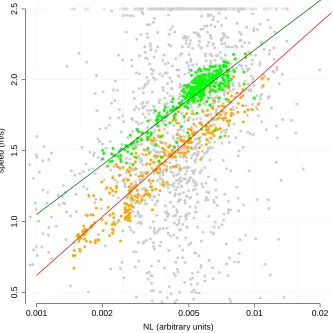
v(t), and consequently speed computed from accelerometer, magnetometer, and depthmeter data could be misleading. One could, however, use Equation (S2–1) to compute a reliable estimate of the speed norm from accelerometer, magnetometer, and depthmeter for periods of high pitch when the equal pitch assumption is likely to hold. As Simon et al. (2009), we consider the section of the dive when the animal is fluking and steeply descends from the sea surface to reach the foraging depth, and hence when the equal pitch assumption is most likely to hold. We apply equation (S2–1) to all samples (n= 384) during the animal descent for which the pitch is greater than 60◦ (an arbitrary threshold).
Background acoustic noise level is expected to increase with animal speed as a consequence of water flow on the sensor. Figure S2.1 shows the observed relationship between estimated speed for the above data versus measured noise level on the tag (on a logarithmic scale). An ordinary linear regression yielded the relationship, for data from descent with pitch>60◦ofE{v(t)}= 4.53 + 1.16 log10(NL(t)), with a residual standard errorσv = 0.08 m/s (R2 =
0.77). The fit is shown in Figure S2.1.
Also shown in Figure S2.1 are the samples (n= 330) during the animal ascent for which the pitch is greater than 60◦. A similar regression on these data yielded somewhat different regression parameters (E{v(t)} = 4.73 + 1.37 log10(NL(t)), with a residual standard errorσv= 0.12 m/s,R2= 0.84).
from the animal’s axis (Figure S2.2: on two occasions a positive pitch, i.e. head oriented upwards, is observed concurrently with a negative vertical speed, i.e. animal moving downwards). We hypothesize that the discrepancy between the descent and ascent calibration results (Figure S2-1) is that for the latter movement direction can differ from the animal’s longitudinal axis. We therefore calibrated the speed-noise relationship with descent data, when the animal is actively navigating downwards, to predict animal speed from the noise level for the rest of the dive.