Microsoft Press Excel 2013 Step by Step pdf

(1)

(2)

Microsoft Excel 2013

Step by Step

(3)

Published with the authorization of Microsoft Corporation by: O’Reilly Media, Inc.

1005 Gravenstein Highway North Sebastopol, California 95472

ISBN: 978-0-7356-6939-0

1 2 3 4 5 6 7 8 9 QG 8 7 6 5 4 3

Printed and bound in the United States of America.

Microsoft Press books are available through booksellers and distributors worldwide. If you need support related to this book, email Microsoft Press Book Support at [email protected]. Please tell us what you think of this book at http://www.microsoft.com/learning/booksurvey.

Microsoft and the trademarks listed at http://www.microsoft.com/about/legal/en/us/IntellectualProperty/

Trademarks/EN-US.aspx are trademarks of the Microsoft group of companies. All other marks are property of

their respective owners.

The example companies, organizations, products, domain names, email addresses, logos, people, places, and events depicted herein are fictitious. No association with any real company, organization, product, domain name, email address, logo, person, place, or event is intended or should be inferred.

This book expresses the author’s views and opinions. The information contained in this book is provided without any express, statutory, or implied warranties. Neither the authors, O’Reilly Media, Inc., Microsoft Corporation, nor its resellers, or distributors will be held liable for any damages caused or alleged to be caused either directly or indirectly by this book.

Acquisitions and Developmental Editor: Kenyon Brown Production Editor: Melanie Yarbrough

Editorial Production: Online Training Solutions, Inc. (OTSI) Technical Reviewer: Andy Pope

Indexer: Judith McConville Cover Design: Girvin

Cover Composition: Zyg Group, LLC

(4)

(5)

(6)

Contents v

Working with data and Excel tables

45

Entering and revising data . . . .46

Managing data by using Flash Fill . . . .50

Moving data within a workbook . . . .54

Finding and replacing data. . . .58

Correcting and expanding upon worksheet data. . . .62

Defining Excel tables . . . .67

Key points . . . .72

3

Performing calculations on data

75

Naming groups of data. . . .76

Creating formulas to calculate values . . . .81

Summarizing data that meets specific conditions . . . .90

Working with iterative calculation options and automatic workbook calculation . . . .94

Using array formulas . . . .96

Finding and correcting errors in calculations . . . .99

4

Changing workbook appearance

107

Formatting cells . . . 108

Defining styles . . . .113

Applying workbook themes and Excel table styles . . . .119

Making numbers easier to read. . . 125

Changing the appearance of data based on its value . . . .131

Adding images to worksheets . . . 138

(8)

Contents vii

5

Focusing on specific data by using filters

145

Limiting data that appears on your screen . . . 146

Filtering Excel table data by using slicers. . . .153

Manipulating worksheet data . . . 158

Selecting list rows at random. . . 158

Summarizing worksheets by using hidden and filtered rows. . . 159

Finding unique values within a data set. . . 163

Defining valid sets of values for ranges of cells. . . .166

6

Reordering and summarizing data

173

Sorting worksheet data. . . .174

Sorting data by using custom lists . . . .179

Organizing data into levels. . . 183

Looking up information in a worksheet . . . 189

7

Combining data from multiple sources

195

Using workbooks as templates for other workbooks. . . 196

Linking to data in other worksheets and workbooks. . . 204

Consolidating multiple sets of data into a single workbook. . . 209

8

Analyzing data and alternative data sets

215

Examining data by using the Quick Analysis Lens . . . .216

Defining an alternative data set. . . .219

Defining multiple alternative data sets. . . 223

Analyzing data by using data tables. . . 227

Varying your data to get a specific result by using Goal Seek . . . 230

Finding optimal solutions by using Solver . . . .233

Analyzing data by using descriptive statistics . . . 240

(9)

9

Creating charts and graphics

245

Creating charts . . . .246

Customizing the appearance of charts. . . 254

Finding trends in your data . . . .262

Creating dual-axis charts. . . .265

Summarizing your data by using sparklines . . . .269

Creating diagrams by using SmartArt . . . .273

Creating shapes and mathematical equations . . . .278

10

Using PivotTables and PivotCharts

287

Analyzing data dynamically by using PivotTables . . . 288

Filtering, showing, and hiding PivotTable data . . . 298

Editing PivotTables . . . 307

Formatting PivotTables . . . .313

Creating PivotTables from external data . . . .321

Creating dynamic charts by using PivotCharts . . . .326

11

Printing worksheets and charts

333

Adding headers and footers to printed pages . . . 334

Preparing worksheets for printing. . . 340

Previewing worksheets before printing . . . 343

Changing page breaks in a worksheet. . . 343

Changing the page printing order for worksheets. . . 345

Printing worksheets . . . 348

Printing parts of worksheets . . . .352

Printing charts. . . .357

(10)

Contents ix

12

Working with macros and forms

361

Enabling and examining macros . . . 362

Changing macro security settings. . . 362

Examining macros . . . 364

Creating and modifying macros . . . 369

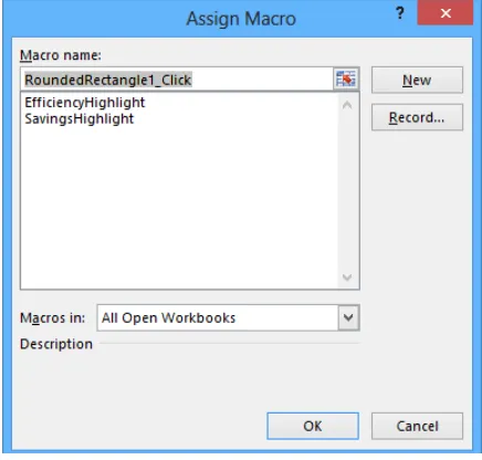
Running macros when a button is clicked . . . .372

Running macros when a workbook is opened . . . .376

Inserting form controls and setting form properties . . . .379

Adding text boxes to UserForms. . . 379

Adding list boxes to UserForms. . . 380

Adding combo boxes to UserForms . . . 381

Adding option buttons to UserForms. . . 381

Adding graphics to UserForms . . . 383

Adding spin buttons to UserForms . . . 384

Writing UserForm data to a worksheet . . . 385

Displaying, loading, and hiding UserForms. . . 386

13

Working with other Office programs

393

Linking to Office documents from workbooks . . . 394

Embedding workbooks into other Office documents . . . 398

Creating hyperlinks . . . 401

Pasting charts into other Office documents . . . 407

(11)

14

Collaborating with colleagues

411

Sharing workbooks . . . .412

Saving workbooks for electronic distribution . . . .416

Managing comments. . . .418

Tracking and managing colleagues’ changes . . . .420

Protecting workbooks and worksheets . . . .424

Authenticating workbooks . . . .433

Saving workbooks as web content . . . .436

Importing and exporting XML data . . . 441

Working with SkyDrive and Excel Web App . . . 446

Glossary. . . 453

Keyboard shortcuts . . . 457

Ctrl combination shortcut keys . . . .457

Function keys . . . .459

Other useful shortcut keys . . . 461

Index . . . 465

(12)

Introduction xi

Introduction

Part of the Microsoft Office 2013 suite of programs, Microsoft Excel 2013 is a full-featured spreadsheet program that helps you quickly and efficiently develop dynamic, professional workbooks to summarize and present your data. Microsoft Excel 2013 Step by Step offers a comprehensive look at the features of Excel that most people will use most frequently.

Who this book is for

Microsoft Excel 2013 Step by Step and other books in the Step by Step series are designed for

beginning-level to intermediate-level computer users. Examples shown in the book gener-ally pertain to small and medium businesses but teach skills that can be used in organiza-tions of any size. Whether you are already comfortable working in Excel and want to learn about new features in Excel 2013 or are new to Excel, this book provides invaluable hands-on experience so that you can create, modify, and share workbooks with ease.

How this book is organized

This book is divided into 14 chapters. Chapters 1–4 address basic skills such as identify-ing the different Excel programs, customizidentify-ing the program window, settidentify-ing up workbooks, managing data within workbooks, creating formulas to summarize your data, and format-ting your workbooks. Chapters 5–10 show you how to analyze your data in more depth through sorting and filtering, creating alternative data sets for scenario analysis, summariz-ing data by ussummariz-ing charts, and creatsummariz-ing PivotTables and PivotCharts. Chapters 11–14 cover printing, working with macros and forms, working with other Microsoft Office programs, and collaborating with colleagues.

(13)

This book has been designed to lead you step by step through all the tasks you’re most likely to want to perform with Excel 2013. If you start at the beginning and work your way through all the exercises, you will gain enough proficiency to be able to create and work with most types of Excel workbooks. However, each topic is self-contained, so you can jump in anywhere to acquire exactly the skills you need.

Download the practice files

Before you can complete the exercises in this book, you need to download the book’s prac-tice files to your computer. These pracprac-tice files can be downloaded from the following page:

http://go.microsoft.com/FWLink/?Linkid=275457

IMPORTANT The Excel 2013 program is not available from this website. You should purchase and install that program before using this book.

The following table lists the practice files for this book.

Chapter File

Chapter 1: Getting started with Excel 2013 DataLabels.xlsx ExceptionSummary.xlsx ExceptionTracking.xlsx MisroutedPackages.xlsx PackageCounts.xlsx RouteVolume.xlsx

Chapter 2: Working with data and Excel tables 2013Q1ShipmentsByCategory.xlsx AverageDeliveries.xlsx

DriverSortTimes.xlsx MailingNames.xlsx Series.xlsx

ServiceLevels.xlsx Chapter 3: Performing calculations on data ConveyerBid.xlsx

(14)

Introduction xiii

Chapter File

Chapter 4: Changing workbook appearance CallCenter.xlsx Dashboard.xlsx ExecutiveSearch.xlsx HourlyExceptions.xlsx HourlyTracking.xlsx VehicleMileSummary.xlsx Chapter 5: Focusing on specific data by using filters Credit.xlsx

ForFollowUp.xlsx PackageExceptions.xlsx Slicers.xlsx

Chapter 6: Reordering and summarizing data GroupByQuarter.xlsx ShipmentLog.xlsx ShippingCustom.xlsx ShippingSummary.xlsx Chapter 7: Combining data from multiple sources Consolidate.xlsx

DailyCallSummary.xlsx FebruaryCalls.xlsx FleetOperatingCosts.xlsx JanuaryCalls.xlsx

OperatingExpenseDashboard.xlsx Chapter 8: Analyzing data and alternative data sets 2DayScenario.xlsx

AdBuy.xlsx DriverSortTimes.xlsx MultipleScenarios.xlsx PackageAnalysis.xlsx RateProjections.xlsx TargetValues.xlsx Chapter 9: Creating charts and graphics FutureVolumes_start.xlsx

(15)

Chapter File

Chapter 10: Using PivotTables and PivotCharts Creating.txt Creating.xlsx Editing.xlsx Focusing.xlsx Formatting.xlsx RevenueAnalysis.xlsx Chapter 11: Printing worksheets and charts ConsolidatedMessenger.png

CorporateRevenue.xlsx HourlyPickups.xlsx PickupsByHour.xlsx RevenueByCustomer.xlsx SummaryByCustomer.xlsx Chapter 12: Working with macros and forms PackageWeight.xlsm

PerformanceDashboard.xlsm RunOnOpen.xlsm

VolumeHighlights.xlsm YearlySalesSummary.xlsm Chapter 13: Working with other Office programs 2013YearlyRevenueSummary.pptx

Hyperlink.xlsx LevelDescriptions.xlsx RevenueByServiceLevel.xlsx RevenueChart.xlsx RevenueSummary.pptx SummaryPresentation.xlsx Chapter 14: Collaborating with colleagues CategoryXML.xlsx

(16)

Introduction xv

Your companion ebook

With the ebook edition of this book, you can do the following:

▪

Search the full text

▪

Print

▪

Copy and paste

To download your ebook, please see the instruction page at the back of the book.

Getting support and giving feedback

The following sections provide information about getting help with Excel 2013 or the con-tents of this book and contacting us to provide feedback or report errors.

Errata

We’ve made every effort to ensure the accuracy of this book and its companion con-tent. Any errors that have been reported since this book was published are listed on our Microsoft Press site at oreilly.com:

http://go.microsoft.com/FWLink/?Linkid=275456

If you find an error that is not already listed, you can report it to us through the same page.

If you need additional support, email Microsoft Press Book Support at

[email protected].

(17)

We want to hear from you

At Microsoft Press, your satisfaction is our top priority, and your feedback our most valuable asset. Please tell us what you think of this book at:

http://www.microsoft.com/learning/booksurvey

The survey is short, and we read every one of your comments and ideas. Thanks in advance for your input!

Stay in touch

(18)

(19)

Chapter at a glance

Customize

Customize the Excel 2013 program window, page 13

Modify

Modify workbooks, page 30

Create

Create workbooks, page 25

Merge

(20)

Getting started with

Excel 2013

IN THIS CHAPTER, YOU WILL LEARN HOW TO

▪

Identify the different Excel 2013 programs.

▪

Identify new features of Excel 2013.

▪

Customize the Excel 2013 program window.

▪

Create workbooks.

▪

Modify workbooks.

▪

Modify worksheets.

▪

Merge and unmerge cells.

When you create a Microsoft Excel 2013 workbook, the program presents a blank work-book that contains one worksheet. You can add or delete worksheets, hide worksheets within the workbook without deleting them, and change the order of your worksheets within the workbook. You can also copy a worksheet to another workbook or move the worksheet without leaving a copy of the worksheet in the first workbook. If you and your colleagues work with a large number of documents, you can define property values to make your workbooks easier to find when you and your colleagues attempt to locate them by searching in File Explorer or by using Windows 8 Search.

TIP In Windows 8, File Explorer has replaced Windows Explorer. Throughout this book, this browsing utility is referred to by its Windows 8 name. If your computer is running Windows 7, use Windows Explorer instead.

You can also make Excel easier to use by customizing the Excel program window to fit your work style. If you have several workbooks open at the same time, you can move between the workbook windows quickly. However, if you switch between workbooks frequently, you might find it easier to resize the workbooks so they don’t take up the entire Excel window. If you do this, you can switch to the workbook that you want to modify by clicking the title bar of the workbook you want.

1

(21)

The Microsoft Office User Experience team has enhanced your ability to customize the Excel user interface. If you find that you use a command frequently, you can add it to the Quick Access Toolbar so it’s never more than one click away. If you use a set of commands fre-quently, you can create a custom ribbon tab so they appear in one place. You can also hide, display, or change the order of the tabs on the ribbon.

In this chapter, you’ll get an overview of the different Excel programs that are available and discover features that are available in Excel 2013. You’ll also create and modify workbooks and worksheets, make workbooks easier to find, and customize the Excel 2013 program window.

PRACTICE FILES To complete the exercises in this chapter, you need the practice files contained in the Chapter01 practice file folder. For more information, see “Download the practice files” in this book’s Introduction.

Identifying the different Excel 2013

programs

The Microsoft Office 2013 suite includes programs that give you the ability to create and manage every type of file you need to work effectively at home, business, or school. The programs include Microsoft Word 2013, Excel 2013, Outlook 2013, PowerPoint 2013, Access 2013, InfoPath 2013, Lync 2013, OneNote 2013, and Publisher 2013. You can pur-chase the programs as part of a package that includes multiple programs or purpur-chase most of the programs individually.

With the Office 2013 programs, you can find the tools you need quickly and, because they were designed as an integrated package, you’ll find that most of the skills you learn in one program transfer readily to the others. That flexibility extends well beyond your personal computer. In addition to the traditional desktop Excel program, you can also use Excel 2013 on devices with ARM chips and over the web. The following describes the different Excel 2013 programs that are available to you:

(22)

TIP Office 365 is a cloud-based subscription licensing solution. Some of the Office 365 subscription levels provide access to the full Excel 2013 program, Excel Web App, or both.

▪

Microsoft Excel 2013 RT Microsoft developed an edition of Windows 8 for devices powered by an ARM processor. Devices running this edition of Windows 8, called Windows RT, come with an edition of Office 2013 named Microsoft Office 2013 RT. The Office 2013 RT program suite includes Excel, OneNote, PowerPoint, and Word. Excel 2013 RT takes advantage of ARM devices’ touch screen capabilities by includ-ing Touch Mode. When you enable Touch Mode, the Excel 2013 RT interface changes slightly to make it easier to work with the program by tapping the screen with your finger or a stylus and by providing an on-screen keyboard through which you can enter data. You can also work with Excel 2013 RT by using a physical keyboard, a mouse, and your device’s track pad.

TIP Excel 2013 RT includes almost all of the functionality found in the Excel 2013 full desktop program; the main difference is that Excel 2013 RT does not support macros. If you open a macro-enabled workbook in Excel 2013 RT, the macros will be disabled.

▪

Microsoft Excel 2013 Web App Information workers require their data to be avail-able to them at all times, not just when they’re using their personal computers. To provide mobile workers with access to their data, Microsoft developed Office Web Apps, which include online versions of Excel, Word, PowerPoint, and OneNote. Office Web Apps are available as part of an Office 365 subscription or for free as part of the Microsoft SkyDrive cloud service.

You can use Excel Web App to edit files stored in your SkyDrive account or on a Microsoft SharePoint site. Excel Web App displays your Excel 2010 and Excel 2013 files as they appear in the desktop program and includes all of the functions you use to summarize your data. You can also view and manipulate (but not create) PivotTables, add charts, and format your data to communicate its meaning clearly. Excel Web App also includes the capabilities to share your workbooks online, to em-bed them as part of another webpage, and to create web-accessible surveys that save user responses directly to an Excel workbook in your SkyDrive account.

After you open a file by using Excel Web App, you can choose to continue editing the file in your browser (such as Windows Internet Explorer 10) or open the file in the desktop program. When you open the file in your desktop program, any changes you save are written to the version of the file on your SkyDrive account. This prac-tice means that you will always have access to the most recent version of your file, regardless of where and how you access it.

1

(23)

▪

Microsoft Excel Mobile If you have a Windows Phone 8 device, you can use Excel Mobile to view and manipulate your workbooks. You can create formulas, change the formatting of worksheet cells, sort and filter your data, and summarize your data by using charts. You can also connect your phone to your SkyDrive account, so all of those files will be available even if you don’t have a notebook or other computer to work with at the moment.

Identifying new features of Excel 2013

Excel 2013 includes all of the most useful capabilities included in previous versions of the program. If you’ve used an earlier version of Excel, you probably want to know about the new features introduced in Excel 2013. The following sections summarize the most impor-tant changes from Excel 2010, Excel 2007, and Excel 2003.

If you are upgrading from Excel 2010

For users of Excel 2010, you’ll find that Excel 2013 extends the program’s existing capabili-ties and adds some very useful new ones. The features introduced in Excel 2013 include:

▪

Windows 8 functionality Excel 2013, like all Office 2013 programs, takes full advan-tage of the capabilities of the Windows 8 operating system. When it is running on a computer running Windows 8, Excel embodies the new presentation elements and enables you to use a touch interface to interact with your data.

▪

A window for each workbook Every workbook now has its own program window.

▪

New functions More than 50 new functions are available, which you can use to summarize your data, handle errors in your formulas, and bring in data from online resources.

▪

Flash Fill If your data is in list form, you can combine, extract, or format the data in a cell. When you continue the operation, Excel detects your pattern and offers to extend it for every row in the list.

▪

Quick Analysis Lens Clicking the Quick Analysis action button, which appears next to a selected cell range, displays different ways to visually represent your data. Click-ing an icon creates the analysis instantly.

(24)

▪

Recommended Charts As with Recommended PivotTables, Excel recommends the most suitable charts based on patterns in your data. You can display the suggested charts, click the one you want, and modify it so it’s perfect.

▪

Chart formatting control You can fine-tune your charts quickly and easily. Change the title, layout, or other elements of your charts from a new and interactive interface.

▪

Chart animations When you change the underlying data in a chart, Excel updates your chart and highlights the change by using an animation.

▪

Cloud capability You can now share workbooks stored online or post part of a work-book to your social network by posting a link to the file.

▪

Online presentation capability You can share your workbook and collaborate in real time with others as part of a Microsoft Lync conversation or meeting. You can also allow others to take control of your workbook during the conversation or meeting.

If you are upgrading from Excel 2007

In addition to the features added in Excel 2013, the Excel programming team introduced the following features in Excel 2010:

▪

Manage Excel files and settings in the Backstage view When the User Experience and Excel teams focused on the Excel 2007 user interface, they discovered that several workbook management tasks that contained content-related tasks were sprinkled among the ribbon tabs. The Excel team moved all of the workbook management tasks to the Backstage view, which users can access by clicking the File tab.

▪

Preview data by using Paste Preview With this feature, you can preview how your data will appear in the worksheet before you commit to the paste.

▪

Customize the Excel 2010 user interface The ability to make simple modifications to the Quick Access Toolbar has been broadened to include many more options for changing the ribbon interface. You can hide or display built-in ribbon tabs, change the order of built-in ribbon tabs, add custom groups to a ribbon tab, and create cus-tom ribbon tabs, which can also contain cuscus-tom groups.

▪

Summarize data by using more accurate functions In earlier versions of Excel, the program contained statistical, scientific, engineering, and financial functions that would return inaccurate results in some relatively rare circumstances. The Excel pro-gramming team identified the functions that returned inaccurate results and collabo-rated with academic and industry analysts to improve the functions’ accuracy.

1

(25)

▪

Summarize data by using sparklines In his book Beautiful Evidence (Graphics Press), Edward Tufte describes sparklines as “intense, simple, wordlike graphics.” Spark lines take the form of small charts that summarize data in a single cell. These small but powerful additions to Excel 2010 and Excel 2013 enhance the program’s reporting and summary capabilities.

▪

Filter PivotTable data by using slicers Slicers visually indicate which values appear in a PivotTable and which are hidden. They are particularly useful when you are pre-senting data to an audience that contains visual thinkers who might not be skilled at working with numerical values.

▪

Filter PivotTable data by using search filters Excel 2007 introduced several new ways to filter PivotTables. These filtering capabilities have been extended with the introduction of search filters. With a search filter, you begin entering a sequence of characters that occur in the term (or terms) by which you want to filter. As you enter these characters, the filter list of the PivotTable field displays only those terms that reflect the values entered into the search filter box.

▪

Visualize data by using improved conditional formats The Excel programming team greatly extended the capabilities of the data bar and icon set conditional formats introduced in Excel 2007. The team also enabled you to create conditional formats that refer to cells on worksheets other than the one on which you’re defining the format.

▪

Create and display math equations With the updated equation designer, you can create any equation you require. The editor has several common equations built in, such as the quadratic formula and the Pythagorean theorem, but it also contains numerous templates that you can use to create custom equations quickly.

(26)

If you are upgrading from Excel 2003

In addition to the changes in Excel 2010 and Excel 2013, users upgrading from Excel 2003 will notice several more significant changes:

▪

The ribbon Unlike in previous versions of Excel, in which you hunted through a com-plex toolbar and menu system to find the commands you wanted, you can use the ribbon user interface to find everything you need at the top of the program window.

▪

Larger data collection capability The larger worksheet includes more than 1 million rows and 16,000 columns.

▪

New file format The Excel file format (.xlsx) uses XML and file compression tech-niques to reduce the size of a typical file by 50 percent.

▪

Expanded cell and worksheet formatting Vast improvements have been made to the color management and formatting options found in previous versions of the pro-gram. You can have as many different colors in a workbook as you like, for example, and you can assign a design theme to a workbook.

▪

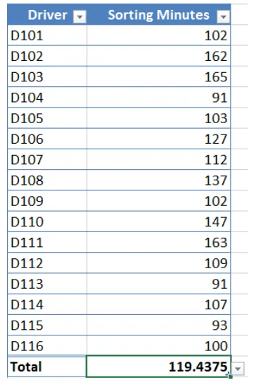
Excel tables These enable you to enter and summarize your data efficiently. If you want to enter data in a new table row, all you have to do is enter the data in the row below the table. When you press Tab or Enter after entering the last cell’s values, Excel expands the table to include your new data. You can also have Excel display a Totals row, which summarizes your table’s data by using a function that you specify.

▪

Improved charting With the charting engine, you can create more attractive charts.

▪

Formula AutoComplete When you enter formulas into an Excel worksheet cell, the program displays a list of options from which you can choose for each formula ele-ment, greatly accelerating formula entry.

▪

Additional formulas With the added formulas, such as AVERAGEIFS, users can sum-marize data conditionally.

▪

Conditional formatting With conditional formats, users can create data bars and color scales, assign icon sets to values, assign multiple conditional formats to a cell, and assign more than three conditional formatting rules to a cell.

1

(27)

Working with the ribbon

As with all Office 2013 programs, the Excel ribbon is dynamic, meaning that as its width changes, its buttons adapt to the available space. As a result, a button might be large or small, it might or might not have a label, or it might even be an entry in a list.

For example, when sufficient horizontal space is available, the buttons on the Home tab are spread out, and the available commands in each group are visible.

If you decrease the horizontal space available to the ribbon, small button labels disappear and entire groups of buttons might hide under one button that represents the entire group. Clicking the group button displays a list of the commands available in that group.

When the ribbon becomes too narrow to display all the groups, a scroll arrow appears at its right end. Clicking the scroll arrow displays the hidden groups.

The width of the ribbon depends on three factors:

(28)

▪

Screen resolution Screen resolution is the size of your screen display expressed as pixels wide × pixels high. Your screen resolution options are dependent on the display adapter installed in your computer, and on your monitor. Common screen resolutions range from 800 × 600 to 2560 × 1600. The greater the number of pixels wide (the first number), the greater the number of buttons that can be shown on the ribbon. To change your screen resolution:

1 Display the Screen Resolution control panel item in one of the following ways:

▪

Right-click the Windows desktop, and then click Screen Resolution.

▪

Enter screen resolution in Windows 8 Search, and then click Adjust screen resolution in the Settings results.

▪

Open the Display control panel item, and then click Adjust resolution.

2 On the Screen Resolution page, click the Resolution arrow, click or drag to select the screen resolution you want, and then click Apply or OK.

1

(29)

▪

The magnification of your screen display If you change the screen magnification setting in Windows, text and user interface elements are larger and therefore more legible, but fewer elements fit on the screen. You can set the magnification from 100 to 500 percent.

You can change the screen magnification from the Display page of the Appearance And Personalization control panel item. You can display the Display page directly from Control Panel or by using one of the following methods:

▪

Right-click the Windows desktop, click Personalize, and then in the lower-left corner of the Personalization window, click Display.

▪

Enter display in Windows 8 Search, and then click Display in the Settings results.

(30)

Customizing the Excel 2013

program window

How you use Excel 2013 depends on your personal working style and the type of data collections you manage. The Excel product team interviews customers, observes how dif-fering organizations use the program, and sets up the user interface so that many users won’t need to change it to work effectively. If you do want to change the program window, including the user interface, you can. You can change how Excel displays your worksheets; zoom in on worksheet data; add frequently used commands to the Quick Access Toolbar; hide, display, and reorder ribbon tabs; and create custom tabs to make groups of com-mands readily accessible.

Zooming in on a worksheet

One way to make Excel easier to work with is to change the program’s zoom level. Just as you can “zoom in” with a camera to increase the size of an object in the camera’s viewer, you can use the zoom setting to change the size of objects within the Excel program win-dow. For example, if Peter Villadsen, the Consolidated Messenger European Distribution Center Manager, displayed a worksheet that summarized his distribution center’s package volume by month, he could click the View tab and then, in the Zoom group, click the Zoom button to open the Zoom dialog box. The Zoom dialog box contains controls that he can use to select a preset magnification level or to enter a custom magnification level. He could also use the Zoom control in the lower-right corner of the Excel window.

Clicking the Zoom In control increases the size of items in the program window by 10 per-cent, whereas clicking the Zoom Out control decreases the size of items in the program window by 10 percent. If you want more fine-grained control of your zoom level, you can use the slider control to select a specific zoom level or click the magnification level indica-tor, which indicates the zoom percentage, and use the Zoom dialog box to set a custom magnification level.

The Zoom group on the View tab contains the Zoom To Selection button, which fills the program window with the contents of any selected cells, up to the program’s maximum zoom level of 400 percent.

TIP The minimum zoom level in Excel is 10 percent.

1

(31)

Arranging multiple workbook windows

As you work with Excel, you will probably need to have more than one workbook open at a time. For example, you could open a workbook that contains customer contact information and copy it into another workbook to be used as the source data for a mass mailing you create in Word. When you have multiple workbooks open simultaneously, you can switch between them by clicking the View tab and then, in the Window group, clicking the Switch Windows button and clicking the name of the workbook you want to view.

You can arrange your workbooks on the desktop so that most of the active workbook is shown but the others are easily accessible. To do so, click the View tab and then, in the Window group, click the Arrange All button. Then, in the Arrange Windows dialog box, click Cascade.

(32)

displaying the worksheet that contains the data in the original window and displaying the worksheet with the formula in the new window. When you change the data in either copy of the workbook, Excel updates the other copy. To display two copies of the same work-book, open the workbook and then, on the View tab, in the Window group, click New Window to opens a second copy of the workbook. To display the workbooks side by side, on the View tab, click Arrange All. Then, in the Arrange Windows dialog box, click Vertical and then click OK.

If the original workbook’s name is MisroutedPackages, Excel displays the name MisroutedPackages:1 on the original workbook’s title bar and MisroutedPackages:2 on the second workbook’s title bar.

TROUBLESHOOTING If the controls in the Window group on the View tab don’t affect your workbooks as you expect, you might have a program, such as SkyDrive for PC, open in the background that prevents those capabilities from functioning.

1

(33)

Adapting exercise steps

The screen shots shown in this book were captured at a screen resolution of 1024 × 768, at 100-percent magnification. If your settings are different, the ribbon on your screen might not look the same as the one shown in this book. As a result, exercise instructions that involve the ribbon might require a little adaptation. This book’s instructions use this format:

▪

On the Insert tab, in the Illustrations group, click the Chart button. If the command is in a list, the instructions use this format:

▪

On the Home tab, in the Editing group, click the Find arrow and then, in the

Find list, click Go To.

If your display settings cause a button to appear differently on your screen than it does in this book, you can easily adapt the steps to locate the command. First click the specified tab, and then locate the specified group. If a group has been collapsed into a group list or under a group button, click the list or button to display the group’s commands. If you can’t immediately identify the button you want, point to likely can-didates to display their names in ScreenTips.

This book provides instructions based on traditional keyboard and mouse input methods. If you’re using Excel on a touch-enabled device, you might be giving com-mands by tapping with your finger or with a stylus. If so, substitute a tapping action any time the instructions ask you to click a user interface element. Also note that when the instructions ask you to enter information in Excel, you can do so by typing on a keyboard, tapping in the entry field under discussion to display and use the on-screen keyboard, or even speaking aloud, depending on your computer setup and your personal preferences.

In this exercise, you’ll change a worksheet’s zoom level, zoom to maximize the display of a selected cell range, switch between workbooks, and arrange all open workbooks on your screen.

SET UP

You need the PackageCounts and MisroutedPackages workbooks located in the Chapter01 practice file folder to complete this exercise. Open both workbooks, and then follow the steps.

(34)

2

Select cells B2:C11.

3

On the View tab, in the Zoom group, click the Zoom to Selection button to display the selected cells so that they fill the program window.

4

On the View tab, in the Zoom group, click the Zoom button to open the Zoom

dialog box.

5

Click 100%, and then click OK to return the worksheet to its default zoom level.

1

(35)

6

On the View tab, in the Window group, click the Switch Windows button, and then click PackageCounts to display the PackageCounts workbook.

7

On the View tab, in the Window group, click the Arrange All button to open the

Arrange Windows dialog box.

8

Click Cascade, and then click OK to cascade the open workbook windows.

+

CLEAN UP

_{Close the PackageCounts and MisroutedPackages workbooks, saving your}

changes if you want to.

Adding buttons to the Quick Access Toolbar

As you continue to work with Excel 2013, you might discover that you use certain com-mands much more frequently than others. If your workbooks draw data from external sources, for example, you might find yourself displaying the Data tab and then, in the Connections group, clicking the Refresh All button much more often than the program’s designers might have expected. You can make any button accessible with one click by add-ing the button to the Quick Access Toolbar, located just above the ribbon in the upper-left corner of the Excel program window.

(36)

pane below the Choose Commands From field. Click the control you want, and then click the Add button.

You can change a button’s position on the Quick Access Toolbar by clicking its name in the right pane and then clicking either the Move Up or Move Down button at the right edge of the dialog box. To remove a button from the Quick Access Toolbar, click the button’s name in the right pane, and then click the Remove button. When you’re done making your changes, click the OK button. If you prefer not to save your changes, click the Cancel but-ton. If you saved your changes but want to return the Quick Access Toolbar to its original state, click the Reset button and then click either Reset Only Quick Access Toolbar, which removes any changes you made to the Quick Access Toolbar, or Reset All Customizations, which returns the entire ribbon interface to its original state.

You can also choose whether your Quick Access Toolbar changes affect all your workbooks or just the active workbook. To control how Excel applies your change, in the Customize Quick Access Toolbar list, click either For All Documents to apply the change to all of your workbooks or For Workbook to apply the change to the active workbook only.

1

(37)

If you’d like to export your Quick Access Toolbar customizations to a file that can be used to apply those changes to another Excel 2013 installation, click the Import/Export button and then click Export All Customizations. Use the controls in the dialog box that opens to save your file. When you’re ready to apply saved customizations to Excel, click the Import/Export button, click Import Customization File, select the file in the File Open dialog box, and click Open.

Customizing the ribbon

Excel enhances your ability to customize the entire ribbon by enabling you to hide and dis-play ribbon tabs, reorder tabs disdis-played on the ribbon, customize existing tabs (including tool tabs, which appear when specific items are selected), and create custom tabs.

(38)

To select which tabs appear in the tabs pane on the right side of the screen, click the Customize The Ribbon field’s arrow and then click either Main Tabs, which displays the tabs that can appear on the standard ribbon; Tool Tabs, which displays the tabs that appear when you click an item such as a drawing object or PivotTable; or All Tabs.

TIP The procedures taught in this section apply to both the main tabs and the tool tabs.

Each tab’s name has a check box next to it. If a tab’s check box is selected, then that tab ap-pears on the ribbon. You can hide a tab by clearing the check box and bring the tab back by selecting the check box. You can also change the order in which the tabs are displayed on the ribbon. To do so, click the name of the tab you want to move and then click the Move Up or Move Down arrow to reposition the selected tab.

Just as you can change the order of the tabs on the ribbon, you can change the order in which groups of commands appear on a tab. For example, the Page Layout tab contains five groups: Themes, Page Setup, Scale To Fit, Sheet Options, and Arrange. If you use the Themes group less frequently than the other groups, you could move the group to the right end of the tab by clicking the group’s name and then clicking the Move Down button until the group appears in the position you want.

1

(39)

To remove a group from a built-in tab, click the name of the group in the right pane and click the Remove button. If you remove a group from a built-in tab and later decide you want to put it back on the tab, display the tab in the right pane. Then, click the Choose Commands From field’s arrow and click Main Tabs. With the tab displayed, in the left pane, click the expand control (which looks like a plus sign) next to the name of the tab that con-tains the group you want to add back. You can now click the name of the group in the left pane and click the Add button to put the group back on the selected tab.

The built-in tabs are designed efficiently, so adding new command groups might crowd the other items on the tab and make those controls harder to find. Rather than adding controls to an existing tab, you can create a custom tab and then add groups and commands to it. To create a custom tab, click the New Tab button on the Customize The Ribbon page of the Excel Options dialog box. When you do, a new tab named New Tab (Custom), which con-tains a group named New Group (Custom), appears in the tab list.

You can add an existing group to your new tab by clicking the Choose Commands From field’s arrow, selecting a collection of commands, clicking the group you want to add, and then clicking the Add button. You can also add individual commands to your tab by clicking a command in the command list and clicking the Add button. To add a command to your tab’s custom group, click the new group in the right tab list, click the command in the left list, and then click the Add button. If you want to add another custom group to your new tab, click the new tab, or any of the groups within that tab, and then click New Group.

TIP You can change the order of the groups and commands on your custom ribbon tabs by using the techniques described earlier in this section.

(40)

If you’d like to export your ribbon customizations to a file that can be used to apply those changes to another Excel 2013 installation, click the Import/Export button and then click Export All Customizations. Use the controls in the dialog box that opens to save your file. When you’re ready to apply saved customizations to Excel, click the Import/Export button, click Import Customization File, select the file in the File Open dialog box, and click Open.

When you’re done customizing the ribbon, click the OK button to save your changes or click Cancel to keep the user interface as it was before you started this round of changes. You can also change a tab, or the entire ribbon, back to the state it was in when you installed Excel. To restore a single tab, click the tab you want to restore, click the Reset button, and then click Reset Only Selected Ribbon Tab. To restore the entire ribbon, including the Quick Access Toolbar, click the Reset button and then click Reset All Customizations.

Maximizing usable space in the program window

You can increase the amount of space available inside the program window by hiding the ribbon, the formula bar, or the row and column labels.

To hide the ribbon, double-click the active tab label. The tab labels remain visible at the top of the program window, but the tab content is hidden. To temporarily redisplay the ribbon, click the tab label you want. Then click any button on the tab, or click away from the tab, to rehide it. To permanently redisplay the ribbon, double-click any tab label.

KEYBOARD SHORTCUT Press Ctrl+F1 to hide and unhide the ribbon. For a complete list of keyboard shortcuts, see “Keyboard shortcuts” at the end of this book.

To hide the formula bar, clear the Formula Bar check box in the Show/Hide group on the View tab. To hide the row and column labels, clear the Headings check box in the Show/ Hide group on the View tab.

In this exercise, you’ll add a button to the Quick Access Toolbar and customize the ribbon.

SET UP

You need the PackageCounts workbook located in the Chapter01 practice file folder to complete this exercise. Open the workbook, and then follow the steps.

1

Click the File tab to display the Backstage view, and then click Options to open the

Excel Options dialog box.

2

Click Quick Access Toolbar to display the Customize The Quick Access Toolbar

page.

1

(41)

3

Click the Choose commands from arrow, and then in the list, click Review Tab to display the commands in the Review Tab category in the command list.

4

Click the Spelling command, and then click Add to add the Spelling command to the

Quick Access Toolbar.

5

Click Customize Ribbon to display the Customize The Ribbon page of the Excel Options dialog box.

6

If necessary, click the Customize the Ribbon box’s arrow and click Main Tabs. In the right tab list, click the Review tab and then click the Move Up button three times to move the Review tab between the Insert and Page Layout tabs.

7

Click the New Tab button to create a tab named New Tab (Custom), which appears below the most recently active tab in the Main Tabs list.

8

Click the New Tab (Custom) tab name, click the Rename button, enter My Commands in the Display Name box, and click OK to change the new tab’s name to My Commands.

9

Click the New Group (Custom) group’s name and then click the Rename button. In the Rename dialog box, click the icon that looks like a paint palette (second row, fourth from the right). Then, in the Display name box, enter Formatting, and click

OK to change the new group’s name to Formatting.

(42)

11

In the left tab list, click the Home tab’s expand control, click the Styles group’s name, and then click the Add button to add the Styles group to the My Commands tab.

12

In the left tab list, below the Home tab, click the Number group’s expand control to display the commands in the Number group.

13

In the right tab list, click the Formatting group you created earlier. Then, in the left tab list, click the Number Format item and click the Add button to add the Number Format item to the Formatting custom group.

14

Click OK to save your ribbon customizations, and then click the My Commands tab on the ribbon to display the contents of the new tab.

IMPORTANT The remaining exercises in this book assume that you are using Excel 2013 as it was installed on your computer. After you complete this exercise, you should reset the ribbon to its original configuration so that the instructions in the remaining exercises in the book are consistent with your copy of Excel.

+

CLEAN UP

_{Close all open workbooks, saving your changes if you want to.}

Creating workbooks

Every time you want to gather and store data that isn’t closely related to any of your other existing data, you should create a new workbook. The default workbook in Excel has one worksheet, although you can add more worksheets or delete existing worksheets if you want. Creating a workbook is a straightforward process—you just display the Backstage view, click New, and click the tile that represents the type of workbook you want.

1

(43)

KEYBOARD SHORTCUT Press Ctrl+N to create a blank workbook.

When you start Excel, the program displays the Start experience. With the Start experi-ence, you can select which type of workbook to create. You can create a blank workbook by clicking the Blank Workbook tile or click one of the built-in templates available in Excel. You can then begin to enter data into the worksheet’s cells. You could also open an existing workbook and work with its contents. In this book’s exercises, you’ll work with workbooks created for Consolidated Messenger, a fictional global shipping company. After you make changes to a workbook, you can save it to preserve your work.

(44)

TIP Readers frequently ask, “How often should I save my files?” It is good practice to save your changes every half hour or even every five minutes, but the best time to save a file is whenever you make a change that you would hate to have to make again.

When you save a file, you overwrite the previous copy of the file. If you have made changes that you want to save, but you also want to keep a copy of the file as it was when you saved it previously, you can use the Save As command to specify a name for the new file. To open the Save As dialog box, in the Backstage view, click Save As.

KEYBOARD SHORTCUT Press F12 to open the Save As dialog box.

You can also use the controls in the Save As dialog box to specify a different format for the new file and a different location in which to save the new version of the file. For example, Lori Penor, the chief operating officer of Consolidated Messenger, might want to save an Excel file that tracks consulting expenses as an Excel 2003 file if she needs to share the file with a consulting firm that uses Excel 2003.

After you create a file, you can add information to make the file easier to find when you search by using File Explorer or Windows 8 Search to search for it. Each category of infor-mation, or property, stores specific information about your file. In Windows, you can search for files based on the file’s author or title, or by keywords associated with the file. A file that tracks the postal code destinations of all packages sent from a vendor might have the key-words postal, destination, and origin associated with it.

To set values for your workbook’s built-in properties, you can display the Backstage view, click Info, click Properties, and then click Show Document Panel to display the Document Properties panel below the ribbon. The standard version of the Document Properties panel has fields for the file’s author, title, subject, keywords, category, and status, and any com-ments about the file.

1

(45)

You can also create custom properties by clicking the arrow located to the right of the Document Properties label, and clicking Advanced Properties to open the Properties dialog box. On the Custom page of the Properties dialog box, you can click one of the existing custom categories or create your own by entering a new property name in the Name field, clicking the Type arrow and selecting a data type (for example, Text, Date, Number, or Yes/ No), selecting or entering a value in the Value field, and then clicking Add. If you want to delete an existing custom property, point to the Properties list, click the property you want to get rid of, and click Delete. After you finish making your changes, click the OK button. To hide the Document Properties panel, click the Close button in the upper-right corner of the panel.

When you’re done modifying a workbook, you should save your changes and then, to close the file, display the Backstage view and then click Close. You can also click the Close button in the upper-right corner of the workbook window.

KEYBOARD SHORTCUT Press Ctrl+W to close a workbook.

In this exercise, you’ll close an open workbook, create a new workbook, save the workbook with a new name, assign values to the workbook’s standard properties, and create a custom property.

SET UP

You need the ExceptionSummary workbook located in the Chapter01 practice file folder to complete this exercise. Open the workbook, and then follow the steps.

1

Click the File tab to display the Backstage view, and then click Close to close the

ExceptionSummary workbook.

2

Display the Backstage view, and then click New to display the New page.

3

Click Blank workbook, and then click Create to open a new, blank workbook.

4

Display the Backstage view, click Save As, click Computer, and then click Browse to open the Save As dialog box.

(46)

6

Click the Save button to save your work and close the Save As dialog box.

7

Display the Backstage view, click Info, click Properties, and then click Show Document Panel to display the Document Properties panel.

8

In the Keywords field, enter exceptions, regional, percentage.

9

In the Category field, enter performance.

10

Click the arrow at the right end of the Document Properties button, and then click

Advanced Properties to open the Exceptions2013 Properties dialog box.

11

Click the Custom tab to display the Custom page.

1

(47)

12

In the Name field, enter Performance.

13

In the Value field, enter Exceptions.

14

Click the Add button, and then click OK to save the properties and close the

Exceptions2013 Properties dialog box.

+

CLEAN UP

_{Close the Exceptions2013 workbook, saving your changes if you want to.}

Modifying workbooks

Most of the time, you create a workbook to record information about a particular activity, such as the number of packages that a regional distribution center handles or the average time a driver takes to complete all deliveries on a route. Each worksheet within that work-book should represent a subdivision of that activity. To display a particular worksheet, click the worksheet’s tab on the tab bar (just below the grid of cells).

(48)

new Excel workbooks contain one worksheet; because Consolidated Messenger uses nine regional distribution centers, you would need to create eight new worksheets. To create a new worksheet, click the New Sheet button (which looks like a plus sign in a circle) at the right edge of the tab bar.

When you create a worksheet, Excel assigns it a generic name such as Sheet2, Sheet3, or

Sheet4. After you decide what type of data you want to store on a worksheet, you should

change the default worksheet name to something more descriptive. For example, you could change the name of Sheet1 in the regional distribution center tracking workbook to

Northeast. When you want to change a worksheet’s name, double-click the worksheet’s tab

on the tab bar to highlight the worksheet name, enter the new name, and press Enter.

Another way to work with more than one worksheet is to copy a worksheet from another workbook to the current workbook. One circumstance in which you might consider copying worksheets to the current workbook is if you have a list of your current employees in an-other workbook. You can copy worksheets from anan-other workbook by right-clicking the tab of the sheet you want to copy and, on the shortcut menu, clicking Move Or Copy to open the Move Or Copy dialog box.

1

(49)

TIP When you select the Create A Copy check box, Excel leaves the copied worksheet in its original workbook, whereas clearing the check box causes Excel to delete the worksheet from its original workbook.

After the worksheet is in the target workbook, you can change the worksheets’ order to make the data easier to locate within the workbook. To change a worksheet’s location in the workbook, you drag its sheet tab to the location you want on the tab bar. If you want to remove a worksheet from the tab bar without deleting the worksheet, you can do so by right-clicking the worksheet’s tab on the tab bar and clicking Hide on the shortcut menu. When you want Excel to redisplay the worksheet, right-click any visible sheet tab and then click Unhide. In the Unhide dialog box, click the name of the sheet you want to display, and click OK.

To differentiate a worksheet from others, or to visually indicate groups or categories of worksheets in a multiple-worksheet workbook, you can change the color of a worksheet tab. To do so, right-click the tab, point to Tab Color, and then click the color you want.

TIP If you copy a worksheet to another workbook, and the destination workbook has the same Office Theme applied as the active workbook, the worksheet retains its tab color. If the destination workbook has another theme applied, the worksheet’s tab color changes to reflect that theme. For more information about Office themes, see Chapter 4, “Changing workbook appearance.”

If you determine that you no longer need a particular worksheet, such as one you created to store some figures temporarily, you can delete the worksheet quickly. To do so, right-click its sheet tab, and then right-click Delete.

In this exercise, you’ll insert and rename a worksheet, change a worksheet’s position in a workbook, hide and unhide a worksheet, copy a worksheet to another workbook, change a worksheet’s tab color, and delete a worksheet.

SET UP

You need the ExceptionTracking workbook located in the Chapter01 practice file folder to complete this exercise. Open the workbook, and then follow the steps.

1

On the tab bar, click the New Sheet button to create a new worksheet.

2

Right-click the new worksheet’s sheet tab, and then click Rename to highlight the new worksheet’s name.

3

Enter 2013, and then press Enter.

(50)

5

Enter 2012, and then press Enter.

6

Right-click the 2013 sheet tab, point to Tab Color, and then, in the Standard Colors

palette, click the green swatch to change the 2013 sheet tab to green.

7

On the tab bar, drag the 2012 sheet tab to the right of the Scratch Pad sheet tab.

8

Right-click the 2013 sheet tab, and then click Hide to remove the 2013 sheet tab from the tab bar.

9

Right-click the 2012 sheet tab, and then click Move or Copy to open the Move or Copy dialog box.

10

Click the To book arrow, and then in the list, click (new book).

11

Select the Create a copy check box.

12

Click OK to create a new workbook and copy the selected worksheet into it.

13

On the Quick Access Toolbar, click Save to open the Save As dialog box.

14

In the File name field, enter 2012 Archive, and then press Enter to save the workbook.

15

On the View tab, click the Switch Windows button, and then click ExceptionTracking

to display the ExceptionTracking workbook.

16

On the tab bar, right-click the Scratch Pad sheet tab, and then click Delete. In the dialog box that opens, click Delete to confirm the operation.

17

Right-click the 2012 sheet tab, and then click Unhide to open the Unhide dialog box.

1

(51)

18

Click 2013, and then click OK to close the Unhide dialog box and display the 2013

worksheet in the workbook.

+

CLEAN UP

_{Close the ExceptionTracking workbook and the 2012 Archive workbook,}

saving your changes if you want to.

Modifying worksheets

After you put up the signposts that make your data easy to find, you can take other steps to make the data in your workbooks easier to work with. For example, you can change the width of a column or the height of a row in a worksheet by dragging the column’s right border or the row’s bottom border to the position you want. Increasing a column’s width or a row’s height increases the space between cell contents, making your data easier to read and work with.

(52)

Inserting rows, columns, and cells

Modifying column width and row height can make a workbook’s contents easier to work with, but you can also insert a row or column between cells that contain data to make your data easier to read. Adding space between the edge of a worksheet and cells that contain data, or perhaps between a label and the data to which it refers, makes the workbook’s contents less crowded. You insert rows by clicking a cell and clicking the Home tab on the ribbon. Then, in the Cells group, in the Insert list, click Insert Sheet Rows. Excel inserts a row above the row that contains the active cell. You insert a column in much the same way, by choosing Insert Sheet Columns from the Insert list. When you do this, Excel inserts a column to the left of the active cell.

When you insert a row, column, or cell in a worksheet that has had formatting applied, the Insert Options button appears. When you click the Insert Options button, Excel displays a list of choices you can make about how the inserted row or column should be formatted, as described in the following table.

Option Action

Format Same As Above Applies the formatting of the row above the inserted row to the new row

Format Same As Below Applies the formatting of the row below the inserted row to the new row

Format Same As Left Applies the formatting of the column to the left of the inserted column to the new column

Format Same As Right Applies the formatting of the column to the right of the inserted column to the new column

Clear Formatting Applies the default format to the new row or column

If you want to delete a row or column, right-click the row or column head and then, on the shortcut menu that appears, click Delete. You can temporarily hide rows or columns by selecting those rows or columns and then, on the Home tab, in the Cells group, clicking the Format button, pointing to Hide & Unhide, and then clicking either Hide Rows or Hide Columns. The rows or columns you selected disappear, but they aren’t gone for good as they would be if you’d used Delete. Instead, they have just been removed from the display until you call them back. To return the hidden rows to the display, select the row or column headers on either side of the hidden rows or columns. Then, on the Home tab, in the Cells group, click the Format button, point to Hide & Unhide, and then click either Unhide Rows or Unhide Columns.

1

(53)

IMPORTANT If you hide the first row or column in a worksheet, you must click the Select All button in the upper-left corner of the worksheet (above the first row header and to the left of the first column header) or press Ctrl+A to select the entire worksheet. Then, on the Home tab, in the Cells group, click Format, point to Hide & Unhide, and then click either Unhide Rows or Unhide Columns to make the hidden data visible again.

Just as you can insert rows or columns, you can insert individual cells into a worksheet. To insert a cell, click the cell that is currently in the position where you want the new cell to appear. On the Home tab, in the Cells group, in the Insert list, click Insert Cells to open the Insert dialog box. In the Insert dialog box, you can choose whether to shift the cells sur-rounding the inserted cell down (if your data is arranged as a column) or to the right (if your data is arranged as a row). When you click OK, the new cell appears, and the contents of affected cells shift down or to the right, as appropriate. Similarly, if you want to delete a block of cells, select the cells, and on the Home tab, in the Cells group, in the Delete list, click Delete Cells to open the Delete dialog box—complete with options that you can use to choose how to shift the position of the cells around the deleted cells.

TIP The Insert dialog box also includes options you can click to insert a new row or column; the Delete dialog box has similar options for deleting an entire row or column.

If you want to move the data in a group of cells to another location in your worksheet, select the cells you want to move and point to the selection’s border. When the pointer changes to a four-pointed arrow, you can drag the selected cells to the desired location on the worksheet. If the destination cells contain data, Excel displays a dialog box asking whether you want to overwrite the destination cells’ contents. If you want to replace the existing values, click OK. If you don’t want to overwrite the existing values, click Cancel and insert the required number of cells to accommodate the data you want to move.

(54)

SET UP

You need the RouteVolume workbook located in the Chapter01 practice file folder to complete this exercise. Open the workbook, and then follow the steps.

1

On the May 12 worksheet, select cell A1.

2

On the Home tab, in the Cells group, click the Insert arrow, and then in the list, click

Insert Sheet Columns to create a new column A.

3

In the Insert list, click Insert Sheet Rows to create a new row 1.

4

Click the Insert Options button that appears below the lower-right corner of the selected cell, and then click Clear Formatting to remove the formatting from the new row 1.

5

Right-click the column header of column E, and then click Hide to remove column E

from the display.

6

On the tab bar, click the May 13 sheet tab to display the worksheet of the same name.

7

Click cell B6.

8

On the Home tab, in the Cells group, click the Delete arrow, and then in the list, click

Delete Cells to open the Delete dialog box.

1

(55)

9

If necessary, click Shift cells up, and then click OK. Excel deletes cell B6, moving the cells below it up to fill in the gap.

10

Click cell C6.

11

In the Cells group, in the Insert list, click Insert Cells to open the Insert dialog box.

12

If necessary, click Shift cells down, and then click OK to close the Insert dialog box, create a new cell C6, and move cells C6:C11 down to accommodate the inserted cell.

13

In cell C6, enter 4499, and then press Enter.

14

Select cells E13:F13.

15

Point to the border of the selected cells. When the pointer changes to a four- pointed arrow, drag