Indirect model predictive control strategy with active damping implementation for a direct matrix converter operating at fixed switching frequency

Indirect Model Predictive Control Strategy with

Active Damping Implementation for a Direct Matrix

Converter Operating at Fixed Switching Frequency

M. Rivera Faculty of Engineering Universidad de Talca, Curic´o, Chile

[email protected]

H. Dan

School of Information Science and Engineering Central South University, ChangSha, China

[email protected]

L. Tarisciotti, P. Wheeler

Dep. of Electrical and Electronic Engineering University of Nottingham, Nottingham, UK

[email protected]

Abstract—One of the main drawbacks of the implementation of predictive control in a direct matrix converter is the high com-putational cost and the adequate selection of weighting factors in order to control both input and output sides. In this paper is proposed an indirect model predictive current control strategy enhanced with a fixed switching predictive strategy and an active damping implementation. With all this, the idea is to reduce the computational cost while eliminating the necessity of weighting factors and improving the performance of the full system. The proposed method is based on the fictitiousdc_{-link concept, which}

has been used in the past for the classical modulation and control techniques of the direct matrix converter. Simulated results confirm the feasibility of the proposal demonstrating that it is an alternative method to classical predictive control strategies for the direct matrix converter.

Index Terms—active damping, current control, matrix convert-ers, indirect model predictive control, fictitiousdc_-link.

NOMENCLATURE

i_{s Source current [isAisB isC]}T v_{s Source voltage [vsAvsB vsC]}T i_{i Input current [iA iB iC]}T v_{i Input voltage [vA vB vC]}T

idc Fictitiousdc-link current

vdc Fictitiousdc-link voltage

i_{o Load current [ia ib ic]}T v_{o Load voltage [va vb vc]}T i∗ _{Load current reference [i}∗

a i∗b i∗c]T

Cf Input filter capacitor

Lf Input filter inductor

Rf Input filter resistor

R Load resistance

L Load inductance

I. INTRODUCTION

The direct matrix converter (DMC) can generates sinusoidal input and output currents but also it has regeneration capabil-ity and adjustable input displacement power factor [1], [2]. Compared to the back-to-back converter, the DMC features some advantages in terms of power densities and capacity to work in harsh pressures and temperatures. Venturini is one of the most classical modulation techniques together with Pulse Width Modulation (PWM), Space Vector Modulation (SVM) as well as Direct Torque Control (DTC) and Model Predictive

To solve issues such as computational cost, weighting factor selections, operation at variable switching frequency and resonances on the input filter, this paper proposes an indirect model predictive control (IMPC) strategy working at fixed switching frequency with active damping implementation. The idea is to emulate the DMC as a two stage converter linked by a fictitiousdc-link allowing a separated and parallel control of both input and output stages, avoiding the use of weighting factors and choosing into the cost function a set of optimal vectors and their respective duty cycles to be applied to the converter.

II. MATHEMATICALMODEL OF THEDMC

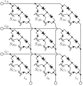
[image:2.612.360.499.66.210.2]

The general structure of the three-phase DMC is shown in Fig. 1. In order to ensure the safe operation of the DMC, the following expression must be accomplished:

SAy + SBy + SCy = 1, ∀ y=a, b, c (1)

The relations between the input and output variables of the DMC are defined by:

v_{o =}T v_{i (2)}

i_i=TTi_{o (3)}

whereT_{is the instantaneous transfer matrix defined as:}

T₌





SAa SBa SCa

SAb SBb SCb

SAc SBc SCc



 (4)

There are some techniques that uses the concept of fictitious

dc-link in order to simplify the modulation and control of the DMC [14], [15], which consists in to divide the converter into a rectifier and an inverter linked by a fictitious dc-link such as represented in Fig. 2. The rectifier have associated six active current space vectors which are represented in Fig. 3 (left) and Table I. The inverter have associated eight voltage space vectors which are represented in Fig. 3 (right) and Table II. The technique modulates both converters separately, but considering the relationship between both stages.

III. PROPOSEDMETHOD FOR THEDMC

M2PC has been implemented in a DMC feeding an in-duction machine [16], [17], where input and output sides of the converter are controlled all together by including a predictive model of the instantaneous reactive input power and a predictive model of the load currents. These predictions are compared with their respective references in a single cost function, being necessary the inclusion of a weighting factor in order to provide more priority to one of the controlled variables. At every sampling period three active and three zero optimal vectors are chosen which are applied to the converter. In this method two main issues are observed: first, it is necessary the adequate selection of a suitable weighting factor value in order to prioritise for the control of the load current or the instantaneous reactive input power and second, as the full converter control is considered, a large amount of available switching states is considered.

iA

iB

iC

ia ib ic

SAa SAb SAc

SBa SBb SBc

SCa SCb SCc

Fig. 1. Power circuit of the direct matrix converter.

[image:2.612.313.544.240.298.2]

DMC _{Fictitious Converter}

Fig. 2. Representation of the fictitiousdc_{-link concept for the DMC.}

α α

β β

i₁

(AC)

i₂

(BC)

i₃

(BA)

i₄

(CA)

i₅

(CB)

i₆

(AB)

v₁

(100)

v₂

(110)

v₃

(010)

v₄

(011)

v₅

(001)

v₆

(101)

v₇

(111)

v₈

(000)

Fig. 3. Current and voltage space vectors of the fictitious converter. Left: current space vectors for the fictitious rectifier, right: voltage space vectors for the fictitious inverter.

TABLE I

VALID SWITCHING STATE ON THE FICTITIOUS RECTIFIER

# Sr1Sr2Sr3Sr4Sr5Sr6 iA iB iC vdc

1 1 1 0 0 0 0 idc 0 -idc vAC

2 0 1 1 0 0 0 0 idc -idc vBC

3 0 0 1 1 0 0 -idc idc 0 -vAB

4 0 0 0 1 1 0 -idc 0 idc -vAC

5 0 0 0 0 1 1 0 -idc idc -vBC

6 1 0 0 0 0 1 idc -idc 0 vAB

TABLE II

VALID SWITCHING STATE ON THE FICTITIOUS INVERTER

# Si1Si2Si3Si4Si5Si6 vab vbc vca idc

1 1 1 0 0 0 1 vdc 0 -vdc ia

2 1 1 1 0 0 0 0 vdc -vdc ia+ib

3 0 1 1 1 0 0 -vdc vdc 0 ib

4 0 0 1 1 1 0 -vdc 0 vdc ib+ic

5 0 0 0 1 1 1 0 -vdc vdc ic

6 1 0 0 0 1 1 vdc -vdc 0 ia+ic

[image:2.612.302.554.330.452.2]

To solve these issues, in this paper we use the concept of fictitious dc-link in order to propose the IMPC strategy for the DMC. The idea is to separate the control of both input and output fictitious stages of the converter in order to avoid complex and large calculations and as well simplify the controller while avoiding the use of weighting factors. In addition, the proposal enhances the performance of the system by the implementation of active damping method in order to mitigate the resonance of the input filter.

A. Control of the Rectifier

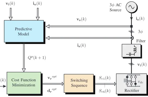
As indicated in Fig. 3 (left) and Table I, there are six active current space vectors which correspond to the suitable switching states of the rectifier. The proposed technique de-tailed in Fig. 4, consists in to control the input side of the converter by considering these available switching states and the mathematical model of the rectifier defined by:

vdc=

Sr1−Sr4 Sr3−Sr6 Sr5−Sr2

v_{i (5)}

i_i=





Sr1−Sr4

Sr3−Sr6

Sr5−Sr2



idc (6)

For the control of the input side it is necessary the prediction model of the source current which is given by the linear model of the input side as:

di_s

dt =

1

Lf

(v_s−v_i)−Rf

Lf

i_{s (7)}

dv_i

dt =

1

Cf

(i_s−i_{i) (8)}

By considering the guidelines presented in [18] for the current and voltage predictions, it is possible to define the cost functiongr associated to the input control in theα-β plane:

gr = [vsα(k+ 1)isβ(k+ 1)−vsβ(k+ 1)isα(k+ 1)]2

(9) At every sampling instantTs, each pair of current vectors

are evaluated for cost functiongr which means that for each

sector two cost functions are given, the first associated to one current vector gr1 and other related to the adjacent current

vector gr2. Later, these cost functions are used to compute

the duty cycles which are calculated assuming that they are proportional to the inverse of the corresponding cost function value, whereKr is a constant to be determined:

dr1 = Kr/gr1

dr2 = Kr/gr2

dr1+dr2 = 1

(10)

With these duty cycles and cost function values, is defined a new cost function which is given by:

grec = dr1gr1+dr2gr2 (11)

This is done, at every sampling time, for each of the six sectors and finally, the pair of vectors that minimizes the cost functiongrecare selected as the optimalvroptto be applied in

Predictive Model

Cost Function Minimization

Filter 3φAC

Source

i_o(k)

Sr1(k) .. .

Sr6(k)

i_s(k)

i_s(k) v_s(k) v_i(k)

v_i(k)

Q∗_(k)

Qp_{(k+ 1)}

3φ

vdc

Rectifier Switching

Sequence

v_ropt

[image:3.612.309.553.67.227.2]

d_ropt

Fig. 4. Indirect predictive control strategy for the fictitious rectifier.

Predictive Model Cost Function

Minimization

i_o(k)

i_o(k) ip

o(k+ 1)

i∗

o(k)

Si1(k) .. .

Si6(k)

v_o(k)

R L

Load 3φ vdc

[image:3.612.322.533.259.436.2]

Fictitious Inverter

Fig. 5. Indirect predictive control strategy for the fictitious inverter.

v_i(k)

v_idq v_dhdq i_dhdq i∗

o(k)

i_out∗dq

θs

SRF

PLL abc

abc dq

dq

Digital dc-blocker

1

[image:3.612.304.555.469.524.2]

Rd +

Fig. 6. Active damping implementation.

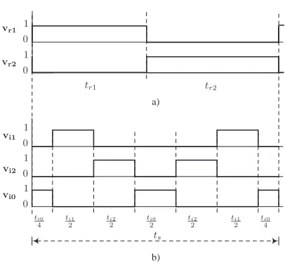
the next period. The time that each vector is applied is given by:

tr1 = dr1Ts

tr2 = dr2Ts

(12)

B. Control of the Inverter

The control diagram of this stage is represented in Fig. 5. The mathematical model of the inverter is defined as:

idc=

Si1 Si3 Si5

i_{o (13)}

v_o=





Si1−Si4

Si3−Si6

Si5−Si2



Assuming a passive RL load, the mathematical model of the load is defined as:

v_o=Ldio

dt +Rio (15)

With these definitions, the prediction model of the output side using a forward Euler approximation in eq. (15) is:

i_{o(k+ 1) =c1}v_{o(k) +c2}i_{o(k) (16)}

where, c1 = Ts/L and c2 = 1 −RTs/L, are constants

dependent on load parameters and the sampling timeTs. The

associated cost functiongi for the output stage is:

gi = [i∗α−iα(k+ 1)]2+ [i∗β−iβ(k+ 1)]2 (17)

In order to enhance the performance of the system and to mitigate the potential resonance of the input filter excited by potential harmonics in the ac source and the converter itself, in this paper we add an active damping technique to the predictive controller of the inverter, by modifying the load current reference as shown in Fig. 6 and indicated in [12], [13]. In this method, we use a virtual harmonic resistive damperRd, which is immune to system parameter variations,

in parallel with the input filter capacitorsCf, to suppress the

system harmonics without affecting the fundamental compo-nent. The converter draws a damping current proportional to the capacitor voltage, which is extracted by the converter itself, emulating the damping resistanceRd as indicated by:

id = v_i

Rd

(18)

This method is easy to implement, do not affects the efficiency of the converter and do not involves additional measurements or any modification to the predictive algorithm. From Fig. 3 (right), six sectors are identified which are given by two active voltage vectors. At every sampling instant Ts,

each pair of voltage vectors and one zero vector are evaluated for cost function gi which means that for each sector three

cost functions are given gi0, gi1 and gi2. Later, these cost

functions are used to compute the duty cycles which are calculated assuming that they are proportional to the inverse of the corresponding cost function value, whereKi is a constant

to be determined:

di0 = Ki/gi0

di1 = Ki/gi1

di2 = Ki/gi2

di0+di1+di2 = 1

(19)

With these duty cycles and cost function values, is defined a new cost function which is given by:

ginv = di1gi1+di2gi2 (20)

This is done, at every sampling time, for each of the six sectors. The pair of vectors that minimizes the cost function

ginv are selected as the optimalvioptto be applied in the next period. The time that each vector is applied is given by:

ti0 = di0Ts

ti1 = di1Ts

ti2 = di2Ts

(21)

ti0 4

ti1 2

ti2 2

ti0 2

ti2 2

ti1 2

ti0 4

ts

tr1 tr2

[image:4.612.325.528.73.262.2]

b) a) 1 1 1 1 1 0 0 0 0 0 v_r1 v_r2 v_i1 vi2 v_i0

Fig. 7. Switching pattern: a) for the rectifier side; b) for the inverter side.

After obtaining the duty cycles and selecting the optimal vectors to be applied in both the rectifier and inverter, a switch-ing pattern procedure is adopted with the goal of applyswitch-ing the optimal vectors [19] (Fig. 7).

C. Relationship between the fictitious converter and the DMC

As it is necessary to apply the switching signals to the switches of the DMC, it is required to adapt the switching states of both input and output fictitious stages to the real one. As indicated in eq. (2), the relationship between the input voltage v_{i and load voltage} v_{o depends on the state of the}

switching given by matrixT_{. Based on the fictitious definition,}

the load voltage v_{o is given as indicated in eq. (14). At the}

same time, the fictitious dc-link voltage vdc is given by eq.

(5). In summary,

v_o=





Si1−Si4

Si3−Si6

Si5−Si2





Sr1−Sr4 Sr3−Sr6 Sr5−Sr2 vi (22) and thus the relationship between the switches of the DMC and fictitious converter is given as:

              SAa SBa SCa SAb SBb SCb SAc SBc SCc               =              

(Si1−Si4)(Sr1−Sr4) (Si1−Si4)(Sr3−Sr6) (Si1−Si4)(Sr5−Sr2) (Si3−Si6)(Sr1−Sr4) (Si3−Si6)(Sr3−Sr6) (Si3−Si6)(Sr5−Sr2) (Si5−Si2)(Sr1−Sr4) (Si5−Si2)(Sr3−Sr6) (Si5−Si2)(Sr5−Sr2)

              (23)

IV. RESULTS

To validate the effectiveness of the proposed method, simu-lation results in Matlab-Simulink were carried out considering

Cf=21 [µF], Lf=400 [µH], Rf=0.5 [Ω], R=10 [Ω], L=10

(a)

(b)

Time [s]

0.02 0.03 0.04 0.05 0.06 0.07 0.08 0.09 0.1

0.02 0.03 0.04 0.05 0.06 0.07 0.08 0.09 0.1

[image:5.612.308.550.67.263.2]

-30 -20 -10 0 10 20 30 -30 -20 -10 0 10 20 30

Fig. 8. Simulation results of the classical MPC; beforet= 0.06_{[s] without} active damping, aftert= 0.06_{[s] with active damping: (a) source voltage} vsA[V/10] and source currentisA[A]; (b) capacitor voltagevA[V/10] and

input currentiA[A].

(a)

(b)

Time [s]

0.02 0.03 0.04 0.05 0.06 0.07 0.08 0.09 0.1

0.02 0.03 0.04 0.05 0.06 0.07 0.08 0.09 0.1

-400 -200 0 200 400 -10 0 10

Fig. 9. Simulation results of the classical MPC; beforet= 0.06_{[s] without} active damping, aftert= 0.06_{[s] with active damping: (a) load currentsi}o

[A] and its respective referencesio∗[A]; (b) load voltageva[V].

In this paper two cases are presented. First the classical MPC with and without active damping implementation is presented followed by the proposal with and without active damping technique.

Fig. 8 and Fig. 9 show simulated results for the classical MPC technique for the DMC with and without active damping implementation. Before the implementation of active damping technique, Fig. 8(a) shows the source voltagevsA and source

current isA which is in phase to its respective voltage but

as expected and due to the variable switching frequency it presents several oscillations and distortions with a THD of 66.95%. This resonance is also reflected in the capacitor voltagevA shown in Fig. 8(b).

(a)

(b)

Time [s]

0.02 0.03 0.04 0.05 0.06 0.07 0.08 0.09 0.1

0.02 0.03 0.04 0.05 0.06 0.07 0.08 0.09 0.1

[image:5.612.44.287.67.264.2]

-30 -20 -10 0 10 20 30 -30 -20 -10 0 10 20 30

Fig. 10. Simulation results of the proposed IMPC; beforet= 0.06_{[s] without} active damping, after t= 0.06_{[s] with active damping: (a) source voltage} vsA[V/10] and source currentisA[A]; (b) capacitor voltagevA[V/10] and

input currentiA[A].

(a)

(b)

Time [s]

0.02 0.03 0.04 0.05 0.06 0.07 0.08 0.09 0.1

0.02 0.03 0.04 0.05 0.06 0.07 0.08 0.09 0.1

-400 -200 0 200 400 -10 0 10

Fig. 11. Simulation results of the proposed IMPC; beforet= 0.06_{[s] without} active damping, aftert= 0.06_{[s] with active damping: (a) load currentsi}o

[A] and its respective references io∗[A]; (b) load voltageva[V].

After the implementation of active damping, the source currentisA is improved and the THD is reduced to 10.62%.

In Fig. 8 is also evident the effect of the input filter which mitigates the high harmonic components of the input currents due to the commutations. Fig. 9(a) shows the load currentsi_o

which track very well their respective references i_o∗ _which

[image:5.612.308.551.323.521.2] [image:5.612.46.287.323.520.2]

As shown in Fig. 10(a), despite of the operation at fixed switching frequency, there is still an oscillation in the source current with a THD of 13.71%which is reduced to 4.30%with the active damping technique. This effect is also observed in Fig. 10(b) where the capacitor voltagevApresents a better

si-nusoidal waveform in comparison to the classical MPC. Again, it is obtained a good performance of the input filter because the high order harmonics produced by the commutation of the switches are eliminated. Fig. 11 show the results on the load side of the DMC where is observed a very good tracking of the load currentsi_{o to their respective references}i_o∗ _{with lower}

ripple in comparison to the classical MPC implementation. Before the implementation of active damping the THD of the load currents is equal to 0.84% and after that it is equal to 0.87%.

V. CONCLUSION

In this paper has been presented an indirect model predictive current control strategy with minimization of the instantaneous reactive input power for a direct matrix converter operating at fixed switching frequency which has been enhanced with an active damping method to reduce the resonance of the input filter. The method uses the idea of fictitiousdc-link in order to separate the control of both input and output stages of the converter. By doing this, it is possible to reduce the complexity of the control, the operation at fixed switching frequency but also avoid the calculation of a suitable weighting factor for the control of both instantaneous reactive input power and load currents variables. By considering the proposed strategy, a new alternative has emerged for the control of both the input and load currents in a direct matrix converter.

ACKNOWLEDGMENTS

The authors would like to thank the financial support of Programa en Energ´ıas CONICYT - Ministerio de Energ´ıa ENER20160014 and FONDECYT Regular 1160690 Research Project.

REFERENCES

[1] L. Empringham, J. Kolar, J. Rodriguez, P. Wheeler, and J. Clare, “Technological issues and industrial application of matrix converters: A review,” Industrial Electronics, IEEE Transactions on, vol. 60, no. 10, pp. 4260–4271, Oct 2013.

[2] J. Rodriguez, M. Rivera, J. Kolar, and P. Wheeler, “A review of control and modulation methods for matrix converters,” Industrial Electronics,

IEEE Transactions on, vol. 59, no. 1, pp. 58–70, Jan 2012.

[3] S. A. Davari, D. A. Khaburi, and R. Kennel, “An improved fcs-mpc algorithm for an induction motor with an imposed optimized weighting factor,” IEEE Transactions on Power Electronics, vol. 27, no. 3, pp. 1540–1551, March 2012.

[4] C. A. Rojas, J. Rodriguez, F. Villarroel, J. R. Espinoza, C. A. Silva, and M. Trincado, “Predictive torque and flux control without weighting factors,” IEEE Transactions on Industrial Electronics, vol. 60, no. 2, pp. 681–690, Feb 2013.

[5] M. Uddin, S. Mekhilef, M. Rivera, and J. Rodriguez, “Predictive indirect matrix converter fed torque ripple minimization with weighting factor optimization,” in 2014 International Power Electronics Conference

(IPEC-Hiroshima 2014 - ECCE ASIA), May 2014, pp. 3574–3581.

[6] Y. Zhang and H. Yang, “Two-vector-based model predictive torque control without weighting factors for induction motor drives,” IEEE

Transactions on Power Electronics, vol. 31, no. 2, pp. 1381–1390, Feb

2016.

[7] V. P. Muddineni, A. K. Bonala, and S. R. Sandepudi, “Enhanced weighting factor selection for predictive torque control of induction motor drive based on vikor method,” IET Electric Power Applications, vol. 10, no. 9, pp. 877–888, 2016.

[8] L. Tarisciotti, A. Formentini, A. Gaeta, M. Degano, P. Zanchetta, R. Rabbeni, and M. Pucci, “Model predictive control for shunt active filters with fixed switching frequency,” IEEE Transactions on Industry

Applications, vol. 53, no. 1, pp. 296–304, Jan 2017.

[9] S. A. Odhano, A. Formentini, P. Zanchetta, R. Bojoi, and A. Tenconi, “Finite control set and modulated model predictive flux and current control for induction motor drives,” in IECON 2016 - 42nd Annual

Conference of the IEEE Industrial Electronics Society, Oct 2016, pp.

2796–2801.

[10] H. Huisman, M. Roes, and E. Lomonova, “Continuous control set space vector modulation for the 3x3 direct matrix converter,” in 2016 18th

European Conference on Power Electronics and Applications (EPE’16 ECCE Europe), Sept 2016, pp. 1–10.

[11] J. Lei, B. Zhou, J. Wei, J. Bian, Y. Zhu, J. Yu, and Y. Yang, “Predictive power control of matrix converter with active damping function,” IEEE

Transactions on Industrial Electronics, vol. 63, no. 7, pp. 4550–4559,

July 2016.

[12] M. Rivera, J. Rodriguez, B. Wu, J. Espinoza, and C. Rojas, “Current control for an indirect matrix converter with filter resonance mitigation,”

Industrial Electronics, IEEE Transactions on, vol. 59, no. 1, pp. 71–79,

Jan 2012.

[13] M. Rivera, C. Rojas, J. Rodridguez, P. Wheeler, B. Wu, and J. Espinoza, “Predictive current control with input filter resonance mitigation for a direct matrix converter,” Power Electronics, IEEE Transactions on, vol. 26, no. 10, pp. 2794 –2803, oct. 2011.

[14] J. Rodriguez, “A new control technique for ac-ac converters,” IFAC

Con-trol in Power Electronics and Electrical Drives, Lausanne Switzerland,

pp. 203–208, 1983.

[15] P. Wheeler, J. Rodriguez, J. Clare, L. Empringham, and A. Weinstein, “Matrix converters: a technology review,” Industrial Electronics, IEEE

Transactions on, vol. 49, no. 2, pp. 276–288, Apr 2002.

[16] M. Vijayagopal, L. Empringham, L. de Lillo, L. Tarisciotti, P. Zanchetta, and P. Wheeler, “Control of a direct matrix converter induction motor drive with modulated model predictive control,” in 2015 IEEE Energy

Conversion Congress and Exposition (ECCE), Sept 2015, pp. 4315–

4321.

[17] ——, “Current control and reactive power minimization of a direct matrix converter induction motor drive with modulated model predictive control,” in 2015 IEEE International Symposium on Predictive Control

of Electrical Drives and Power Electronics (PRECEDE), Oct 2015, pp.

103–108.

[18] C. F. Garcia, M. E. Rivera, J. R. Rodr´ıguez, P. W. Wheeler, and R. S. Pe˜na, “Predictive current control with instantaneous reactive power minimization for a four-leg indirect matrix converter,” IEEE

Transactions on Industrial Electronics, vol. 64, no. 2, pp. 922–929, Feb

2017.

[19] S. Vazquez, A. Marquez, R. Aguilera, D. Quevedo, J. Leon, and L. Franquelo, “Predictive optimal switching sequence direct power control for grid connected power converters,” Industrial Electronics,