Bank Capital Requirements and Collateralised Lending Markets
Margarita Rubio
University of Nottingham
José A. Carrasco-Gallegoy
University of Portsmouth
September 2016
Abstract
In this paper, we take as a baseline a dynamic stochastic general equilibrium (DSGE) model,
which features a housing market, borrowers, savers and banks, in order to evaluate the welfare and
macroeconomic e¤ects of the new …xed capital requirements in the Basel accords. Our results show
that the higher capital requirements imposed by Basel I, II and III decrease both the quantity of
borrowing and its variability, producing distributional welfare e¤ects among agents: savers are better
o¤, but borrowers and banks are worse o¤. Then, we propose a macroprudential rule for the
counter-cyclical capital bu¤er of Basel III in which capital requirements respond to credit growth, output and
housing prices. We …nd that the optimal implementation of Basel III is countercyclical for borrowers
and banks, the agents directly a¤ected by capital requirements, while procyclical for savers. From a
normative perspective, we see that this macroprudential rule for Basel III delivers higher welfare for
the society than a situation with no regulation.
Keywords: Basel I, Basel II, Basel III, banking regulation, welfare, banking supervision,
macro-prudential, capital requirement ratio, credit, countercyclical capital bu¤er.
JEL Classi…cation: E32, E44, E58
University of Nottingham, University Park, Sir Clive Granger Building, Nottingham. e-mail. mar-garita.rubio@nottingham.ac.uk.
yUniversity of Portsmouth, Portland St, Portsmouth PO1 3DE, UK. E-mail: jose.carrasco-gallego@port.ac.uk. This
"The …nancial crisis brought home the lesson that …nancial stability could not be assured only through
the use of microprudential tools. And so Basel III represents another important step in the Committee’s development. Basel III has substantially enhanced the microprudential framework. And, in the counter-cyclical bu¤ er, it has also introduced the …rst international agreement on a macroprudential tool". Stefan Ingves, Chairman of the Basel Committee on Banking Supervision and Governor of Sveriges Riksbank, at
a symposium to mark 25 years of the Basel Capital Accord: 25 years of international …nancial regulation:
Challenges and opportunities, Basel, 26 September 2013.
1
Introduction
After the introduction of new bank capital regulations by the Basel accords, there exists a continuing
public policy concern about the macroeconomic impact of these codes of practice, especially in the
aftermath of the …nancial crisis. In this paper, we perform an analysis of the impact of …xed capital
requirements corresponding to Basel I, II, and III in a DSGE model featuring a housing market and
a …nancial intermediary.1 We contribute to the literature on several fronts. First, we explore the
distributional implications of bank capital requirements imposed by Basel I, II, and III on patient
unconstrained savers, impatient …nancial constrained borrowers, and …nancial intermediaries. While the
literature …nds a small aggregate impact, our results show larger distributional e¤ects: savers are better
o¤ when banks are required to hold more capital, but borrowers and banks are initially worse o¤ with this
measure. Second, we are able to quantify the gains in …nancial stability coming from the regulation, by
taking the variability of borrowing as the closest measure.2 Third, we propose a rule to approximate the
countercyclical capital bu¤er in which the capital requirement responds not only to credit variables but
also to house prices and output. Finally, we contribute to the discussion of the procyclical e¤ects of Basel
III by showing that, for the optimal implementation that we calculate, the regulation is countercyclical
for borrowers and banks while procyclical for savers.
In order to achieve our research goals, we build a dynamic stochastic general equilibrium model
(DSGE). The advantage of using this kind of models is that, since they are general equilibrium, they
can account for the interactions of all the relevant variables in the economy. They are dynamic, and
therefore the e¤ects of di¤erent shocks can be studied. They rely on deep parameters and are, thus,
1The machinery of this paper cannot compare Basel I with Basel II since this would require distinguishing two assets
of di¤erent riskiness in order to introduce the impact of Basel II risk weightings based on the internal ratings-based (IRB) risk curves, and, in this model, there is only one kind of bank lending. Then, Basel I and Basel II are analyzed together.
2
free from the Lucas critique, allowing to analyze counterfactuals and do policy evaluation. And …nally,
since they are microfounded, they are suitable for welfare analysis. In particular, we construct a Real
Business Cycle model (RBC) which relies on technology shocks as the main source of macroeconomic
‡uctuations.3
Our model features borrowers, savers, and …nancial intermediaries. The reason for splitting
house-holds into borrowers and savers is that in this way, in equilibrium, credit is not zero as in a representative
agent problem. Borrowers are constrained in the amount they can borrow while banks are constrained
in the amount they can lend; that is, they have a capital requirement ratio. We study …rst how capital
requirements a¤ect dynamics and welfare. We observe that higher capital requirements decrease the
quantity of borrowing in the economy and that reduces borrowers and banks consumption. In terms of
welfare, savers are better o¤ if capital requirements increase, while borrowers and banks are worse o¤
initially. After a certain threshold, volatility e¤ects prevail for these latter agents and their welfare also
increases.
Then, we propose a macroprudential rule for the capital bu¤er of Basel III. Authorities may emphasize
any variables that make sense to them for purposes of assessing the sustainability of credit growth and the
level of system-wide risk. Some examples of variables that may be useful indicators are asset prices, GDP,
and credit condition indicators. Then, along these lines, we propose a countercyclical macroprudential
rule in which capital requirements respond to credit growth, output and housing prices. Then, we
compute the optimal parameters that maximize welfare. Our results show that the regulator, when
implementing the rule, should attach relatively more weight to output and house prices, rather than to
credit growth, given that the former ones serve as an anticipated indicator of credit growth; when the
regulator observes credit growth itself, it may be too late to avoid it. An optimal implementation of the
macroprudential component of Basel III is welfare improving. Furthermore, the optimal implementation
of Basel III with the countercyclical capital bu¤er is, precisely, countercyclical for banks and borrowers,
the ones directly a¤ected by capital requirements and collateral constraints, but procyclical for savers,
not a¤ected by any friction.
The rest of the paper continues as follows. Section 1.1 makes a review of the literature. Section 2
presents the modeling framework. Section 3 displays simulations. Section 4 studies welfare. Section 5
analyzes the optimal implementation of the countercyclical capital bu¤er of Basel III. Section 6 concludes.
3
1.1 Policy Background and Related Literature
Basel III is a comprehensive set of post-crisis reform measures in banking regulation, supervision and
risk management. It was developed by the Basel Committee on Banking Supervision (BCBS) at the
Bank for International Settlements (BIS), to strengthen the banking sector and achieve …nancial
stabil-ity. Furthermore, some of the new measures that Basel III introduces are aimed at preventing future
crises, creating a sound …nancial system in which …nancial problems are not spread to the real
econ-omy. Preventive measures acting in this direction are known between researchers and policy-makers as
"macroprudential policies."
The BCBS seeks to deliver some guidance for banking regulators on what the best practice for banks
is. Its standards are accepted worldwide and are generally incorporated in national banking regulations.
Basel I, signed in 1988, was the …rst accord on the issue. Basel I primarily focused on credit risk:
banks with international presence were required to hold capital equal to 8 % of the risk-weighted assets.
Basel II, initially published in June 2004, was intended to create an international standard for banking
regulators to control how much capital banks need to put aside to guard against the types of …nancial and
operational risks banks and the whole economy face. The BCBS issued a new agreement in 2010, known
as the Basel III Accord, to increase the resilience of the system and to prevent the occurrence of a …nancial
crisis in the future. This new accord introduces a mandatory capital conservation bu¤er of 2.5% designed
to enforce corrective action when a bank’s capital ratio deteriorates. Then, although the minimum total
capital requirement remains at the current 8% level, yet the required total capital increases up to 10.5%
when combined with the conservation bu¤er. Furthermore, it also adds a macroprudential element in
the form of a countercyclical capital bu¤er up to another 2.5% of capital, which asks banks to hold more
capital in good times to prepare for inevitable downturns in the economy. In this way, Basel III tries to
achieve the broader macroprudential goal of reducing systemic risk, which in turns protects the banking
sector from periods of excessive credit growth.
Our work is related with the literature which emphasizes the externalities associated with bank
lending and credit and in particular through the price of collateral. For instance, Lorenzoni (2008)
and Bianchi (2011) highlight that when individual …nancial institutions borrow, they may not take into
account the possibility that their action could depress collateral values and hence tighten the borrowing
constraints throughout the system. In this spirit, the macroprudential tool that we propose for the
externalities arising from the behavior of individual institutions as well as the structure of the …nancial
system. This tool may face the ex-ante externalities that lead to an excessive build-up of systemic risk,
and the ex-post externalities that can generate ine¢ cient failures of institutions in a crisis. As well,
Aikman et al. (2010) and Aikman et al. (2012) consider that banks may have incentives to undertake
excessive lending due to strategic complementarities (reputational concerns, for instance) when other
banks are pro…table and are expanding lending. Therefore, an increase in our countercyclical capital
bu¤er during a credit boom would improve resilience directly by enhancing the loss-absorbing capacity
of the system because it would tighten the constraint on …nancial institutions, such that they cannot
increase their risk-weighted assets beyond a certain multiple of equity capital. This policy action could
in some circumstances, as Giese et al. (2013) describe, raise the funding costs of …nancial institutions.
When higher funding costs translate into higher lending rates, credit growth would slow down. In
addition to increasing banks’ capacity to absorb losses, stricter capital requirements might therefore
help moderate an unsustainable credit boom, thereby reducing the probability of a crisis
The seminal contribution by Kiyotaki and Moore (1997) stress that collateralized borrowing hinges
on market values, yet such market values are endogenous to the economy and out of control by creditors
and debtors. In that line of research, the recent work of Pintus et al. (2015) point out that the market
value of collateral generates an externality that serves to amplify and propagate business cycle shocks.
We …nd that this externality can be used in a countercyclical way for macroprudential purposes. That is,
we use this externality to control the cycle via a macroprudential tool based on the price of collateral. For
instance, when the economy is overheated, the macroprudential tool can let the market value of collateral
to be below trend, collateralized borrowing restricts credit lending, and, thanks to the externality, this
creates a downturn.
Our paper is also connected as well with the literature that uses a DSGE model to study the e¤ects of
a macroprudential rule, given the macroprudential ‡avor of Basel III. For instance, Antipa et al. (2010)
use a DSGE model to show that macroprudential policies would have been e¤ective in smoothing the
past credit cycle and in reducing the intensity of the recession. Some of the scholars have used this type
of models to study the loan-to-value ratio (LTV) as a macroprudential tool, such as Kannan et al. (2012)
or Rubio and Carrasco-Gallego (2015), among others. In our paper, we also use a DSGE framework to
evaluate the capital requirement ratios of Basel I and II (8%) and Basel III (10.5%) plus the optimal
parameterization of the countercyclical capital bu¤er as a macroprudential tool. Our strategy can be
We use this framework to evaluate the compulsory capital requirement ratios of Basel I, II and III and
the countercyclical capital bu¤er that this latter regulation proposes.
This setting lets us add some light to the discussion about capital regulation that the recent …nancial
crisis put at the forefront. Even the BCBS recognizes a negative but low e¤ect on economic growth
although considers that the bene…ts from reducing the probability of …nancial crises and the output
losses associated with such crises are larger (see BCBS, 2010). In this line, some policy-makers and
scholars argue in favour of a substantial increase in capital requirements (see, e.g., Admati et al., 2013)
because of the positive welfare e¤ects. Albeit, others claim that a more restrictive bank regulation might
have negative impact for credit extension and growth (see, e.g., Adrian and Ashcraft, 2012). The welfare
evaluation that we develop is a complete welfare analysis for the di¤erent agents of the economy that
lets a better understanding of a change in the capital requirement ratio because it disentangles the level
and volatility e¤ects for each agent. We …nd that the distributional impacts are relatively large, even
when the aggregate welfare e¤ects are small, because there is a welfare trade-o¤ between borrowers and
savers.
We also contribute by proposing a macroprudential rule for the capital bu¤er of Basel III. Before us,
other academics have analyzed this capital bu¤er with a DSGE framework and proposed some rules. For
instance, Kannan et al. (2012) assume that policy-makers can a¤ect the market lending rate by imposing
additional capital requirements or additional provisioning when credit growth is above its steady-state
value. Angelini et al. (2014) introduce a time-varying capital ratio that adjusts the requirements only in
response to movements in the loans-to-output ratio. We propose a macroprudential rule for the capital
bu¤er of Basel III in which capital requirements respond to credit growth, output and house prices. We
believe that these three variables are able to capture the spirit of BCBS (2010) that considers that useful
indicators of assessing the sustainability of credit growth and the level of system-wide risk are asset
prices, GDP, and credit condition indicators. Drehmann et al. (2010) also point out that the deviations
of credit from its long-term trend are very good indicators of the increase in systemic risk, which is the
macroprudential attention. We …nd the optimal parameters of the rule that maximize welfare and see
that the regulator should attach relatively more weight to the output and the house price parameters in
the rule, rather than to the credit growth parameter, given that they serve as an anticipated indicator
of credit growth. Our results are in line of Jiménez et al.(2014) who empirically show that building
up capital bu¤ers before a crisis occurs is superior in terms of maintaining real activity and avoiding
macroprudential component of Basel III delivers higher welfare for the society than a situation with no
regulation.
With this paper, we add some new insights to the analysis of the cyclicality of the new regulation. Our
model dynamics show that, using the optimized parameters for the macroprudential capital bu¤er, after
an expansionary shock, when GDP is going up, the regulator increases capital requirements. This, in
turn, cuts borrowing, and achieves the goal of the regulation, which is to avoid excessive credit growth. A
number of other studies have also found that increasing capital requirements may reduce credit supply
(Kishan and Opiela, 2000; Gambacorta and Mistrulli, 2004). In the same line, Akram (2014) …nds
that the proposed increases in capital requirements under Basel III are found to have signi…cant e¤ects
especially on house prices and credit. Our results are related to Drehmann and Gambacorta (2011) which
show a simulation that indicates that the countercyclical bu¤er scheme might reduce credit growth during
credit booms and decrease the credit contraction once the bu¤er is released. This would help to achieve
higher banking sector resilience to shocks. Nevertheless, their procedure is subject to the Lucas critique:
had the scheme been in place, banks’ lending decisions would probably have been di¤erent. However,
our approach is robust to this critique because is based on a DSGE model.
There also exists some controversy around this regulation that has been pointed out by the literature.
In particular, some concerns have been raised about the impact of Basel III reforms on the dynamism
of …nancial markets and, in turn, on investment and economic growth. The reasoning is that Basel III
regulation could produce a decline in the amount of credit and impact negatively in the whole economy.
Critics of Basel III consider that there is a real danger that this reform will limit the availability of
credit and reduce economic activity. Repullo and Saurina (2012) show that a mechanical application of
Basel III regulation would tend to reduce capital requirements when GDP growth is high and increase
them when GDP growth is low. Then, if banks increase capital requirements during crises, credit will
be reduced and the economic growth will be even lower; with a lower growth, welfare will decrease.
This is the so-called risk of procyclicality, that is, Basel III could cause a deeper recession in bad times
and a higher boom in good ones. Furthermore, it could have an adverse impact on growth plans of the
industry, as pointed out by Kant and Jain (2013). If capital requirement ratios increase, households
and industries cannot borrow as much, and their plans for recovery would be a¤ected, having an impact
on the whole economy. Some authors have attempted to evaluate the e¤ects of capital ratios such as
Angeloni and Faia (2013) and Repullo and Suárez (2013). They compare the procyclicality of Basel II
paper, we add to this discussion. Our results show that the e¤ect is countercyclical for borrowers and
banks, the agents directly a¤ected by capital requirements, while procyclical for savers.
2
Model Setup
The economy features patient and impatient households, banks and a …nal goods …rm. Households
work and consume both consumption goods and housing. Patient and impatient households are savers
and borrowers, respectively. Financial intermediaries intermediate funds between consumers. Banks are
credit constrained in how much they can borrow from savers, and borrowers are credit constrained with
respect to how much they can borrow from banks. The representative …rm converts household labor
into the …nal good.
2.1 Savers
Savers maximize their utility function by choosing consumption, housing and labor hours:
maxE0
1
X
t=0
t
s logCs;t+jlogHs;t
(Ns;t)
;
where s 2 (0;1) is the patient discount factor, E0 is the expectation operator and Cs;t, Hs;t and
Ns;t represent consumption at time t, the housing stock and working hours, respectively. 1=( 1) is
the labor supply elasticity, >0: j >0constitutes the relative weight of housing in the utility function.
Subject to the budget constraint:
Cs;t+Dt+qt(Hs;t Hs;t 1) =Rs;t 1Dt 1+Ws;tNs;t; (1)
whereDt denotes bank deposits,Rs;t is the gross return from deposits, qt is the price of housing in
units of consumption, andWs;tis the wage rate. The …rst order conditions for this optimization problem
are as follows:
1
Cs;t
= sEt 1
Cs;t+1
Rs;t (2)
qt
Cs;t = j
Hs;t
+ sEt
qt+1
Cs;t+1
(3)
Equation(2)is the Euler equation, the intertemporal condition for consumption, which implies that
savers smooth consumption over time. Equation (3)represents the intertemporal condition for housing,
in which, at the margin, bene…ts for consuming housing equate costs in terms of consumption. Equation
(4) is the labor-supply condition.
2.2 Borrowers
Borrowers solve:
maxE0
1
X
t=0
t
b logCb;t+jlogHb;t
(Nb;t)
;
where b2(0;1)is the impatient discount factor, subject to the budget constraint and the collateral
constraint:4
Cb;t+Rb;tBt 1+qt(Hb;t Hb;t 1) =Bt+Wb;tNb;t; (5)
Bt Et
1
Rb;t+1
kqt+1Hb;t ; (6)
where Bt denotes bank loans and Rb;t is the gross interest rate to be paid by borrowers for their
loans. k can be interpreted as a loan-to-value ratio.5 The borrowing constraint limits borrowing to the
present discounted value of their housing holdings, that is, they use housing as collateral.6 The …rst
order conditions are as follows:
1
Cb;t
= bEt 1
Cb;t+1
Rb;t+1 + b;t; (7)
j Hb;t
=Et 1
Cb;t
qt bEt
qt+1
Cb;t+1 b;t
1
Rb;t+1
kqt+1; (8)
4
Our setup is DSGE, since it represents an extension of a simple Real Business Cycle (RBC) model with collateral constraints a-la-Kiyotaki and Moore. The stochastic nature of the model comes from technology shocks, which are the source of business cycle ‡uctuations. As in Kiyotaki and Moore (1997), the introduction of the collateral constraint ensures that debt repayments are always ful…lled and default is ruled out.
5
Rubio and Carrasco-Gallego (2014) …nd that, starting from a value of the LTV of 0.55, there is a trade-o¤ between borrowers and savers in terms of welfare when we keep increasing the LTV. Large values of the LTV harm borrowers while savers bene…t from the increase. Social welfare decreases.
6
Wb;t= (Nb;t) 1Cb;t; (9)
where b;t denotes the multiplier on the borrowing constraint. These …rst order conditions can be
interpreted analogously to the ones of savers with the di¤erence that collateral terms appear in them
re‡ecting wealth e¤ects. Through simple algebra, it can be shown that the Lagrange multiplier is positive
in the steady state and thus the collateral constraint holds with equality.7 This means that borrowers,
unlike savers, cannot smooth consumption because their consumption comes determined by how much
they can borrow.8 This represents the …rst distortion of the model: borrowers do not have free access
to …nancial markets and thus cannot freely smooth consumption.
2.3 Financial Intermediaries
Banks solve the following problem:
maxE0
1
X
t=0
t
f[logDivf;t];
where f 2(0;1)is the …nancial intermediary discount factor and Divf;t are dividends. Subject to
the budget constraint and the collateral constraint:9
Divf;t+Rs;t 1Dt 1+Bt=Dt+Rb;tBt 1; (10)
where the right-hand side measures the sources of funds for the …nancial intermediary; household
deposits and repayments from borrowers on previous loans. The funds can be used to pay back depositors
and to extend new loans, or can be used as dividends. We assume here that dividends are transformed
into consumption by banks, so that Divf;t = Cf;t: As in Iacoviello (2015), we assume that the bank,
by regulation, is constrained by the amount of assets minus liabilities, as a fraction of assets. That is,
there is a capital requirement ratio. We de…ne capital as assets minus liabilities, so that, the fraction of
capital with respect to assets has to be larger than a certain ratio:
7
In this model, as in Iacoviello-type models, low uncertainty and small curvature of the utility function are su¢ cient to guarantee that the borrowing constraint is always binding over the relevant range and therefore there is no negative consumption.
8
As discussed in Iacoviello (2005), the frequency of borrowing constrained periods depends on the loan-to-value ratio.
9In a model without banks and a capital constraint, there would not be any spread between the lending and the deposit
Bt Dt
Bt
CRR: (11)
Simple algebra shows that this relationship can be rewritten as:
Dt (1 CRR)Bt; (12)
If we de…ne = (1 CRR), we can reinterpret the capital requirement ratio condition as a standard
collateral constraint, so that banks liabilities cannot exceed a fraction of its assets, which can be used
as collateral:10
Dt Bt; (13)
where <1. The …rst order conditions for deposits and loans are as follows:
1
Cf;t
= fEt 1
Cf;t+1
Rs;t + f;t; (14)
1
Cf;t
= fEt 1
Cf;t+1
Re;t+1 + f;t; (15)
where f;t denotes the multiplier on the …nancial intermediary’s borrowing constraint. Financial
intermediaries have a discount factor f < s: This condition ensures that the collateral constraint of
the intermediary holds with equality in the steady state, since f = s s f›0.
11 This binding constraint
represents the second distortion of the model. The fact that …nancial intermediaries need to hold a certain
amount of capital determines their dividends and therefore their consumption. Thus, like borrowers, they
are not consumption smoothers.12
Table 1 displays the assets and the liabilities of the di¤erent agents for a better understanding of the
1 0This constraint creates a relationship between capital requirements and the volatility of borrower consumption. Bank
capital constraints provide a substantial bene…t of reducing the sensitivity of consumption to house prices and avoiding …nancial problems.
1 1
In the real world, bank capital reduces moral hazard problems and the probability of a …nancial crisis. However, the model is not able to capture such bene…ts due to the presence of binding borrowing constraints that rule out the possibility of …rms and banks to go in default. However, as Clerc et al. (2014) …nd, using a DSGE model, the probability of default for banks is negligible for capital requirement ratios higher than 10%, in the range of Basel III regulation.
1 2The model without banks reduces to Iacoviello (2005) or Rubio and Carrasco-Gallego (2014). These models are similar
structure of the model.
Table 1: Assets and Liabilities
Savers Borrowers Banks
Assets Liabilities Assets Liabilities Assets Liabilities
Deposits Dt Dt
Borrowing Bt Bt
Housing qtHs;t qtHb;t
Equity Capital (1 )Bt
2.4 Firms
Firms produce the …nal consumption good. The problem for the …nal good …rms is standard and static.
They maximize pro…ts subject to the production function by using labor from both types of households:13
max t=Yt Ws;tNs;t Wb;tNb;t;
Yt=AtNs;tNb;t1 ; (16)
whereAtrepresents a technology parameter. The problem delivers the standard …rst-order conditions,
which represent the labor-demand equations:
Ws;t =
Yt
Ns;t
; (17)
Wb;t=
(1 )Yt
Nb;t
: (18)
2.5 Equilibrium
The total supply of housing is …xed and it is normalized to unity:
Hs;t+Hb;t= 1: (19)
1 3Following the literature that starts with Kiyotaki and Moore (1997) and builds up with Iacoviello (2005) and Iacoviello
The goods market clearing condition is as follows:
Yt=Cs;t+Cb;t+Cf;t; (20)
Labor supply (equations 4 and 9) and labor demand (equations 17 and 18) are equal to each other, so
that labor markets also clear. Equilibrium in …nancial markets is dictated by the regulatory constraint
for banks, that is, Dt= (1 CRR)Bt:
3
Simulation
3.1 Parameter Values
The discount factor for savers, s, is set to 0.99 so that the annual interest rate is 4% in steady state.
The discount factor for the borrowers is set to 0.98.14 As in Iacoviello (2015), we set the discount
factors for the bankers at 0.965 which, together with the bank leverage parameters implies a spread of
about 1 percent (on an annualized basis) between lending and deposit rates. The steady-state weight
of housing in the utility function, j, is set to 0.1 in order for the ratio of housing wealth to GDP to be
approximately 1.40 in the steady state, consistent with the US data. We set = 2, implying a value
of the labor supply elasticity of 1.15 For the parameters controlling leverage, we set k and to 0.90,
which implies a capital requirement ratio of 10%, in line with the US data.16 The labor income share for
savers is set to 0.64, following the estimate in Iacoviello (2005). We assume that technology, At, follows
an autoregressive process with 0:9 persistence and a normally distributed shock. Table 2 presents a
summary of the parameter values used:
1 4
Lawrance (1991) estimated discount factors for poor consumers at between 0.95 and 0.98 at quarterly frequency. We take the most conservative value.
1 5Microeconomic estimates usually suggest values in the range of 0 and 0.5 (for males). Domeij and Flodén (2006) show
that in the presence of borrowing constraints this estimates could have a downward bias of 50%.
Table 2: Parameter Values
s :99 Discount Factor for Savers
b :98 Discount Factor for Borrowers
f :965 Discount Factor for Banks
j :1 Weight of Housing in Utility Function
2 Parameter associated with labor elasticity
k :90 Loan-to-value ratio
CRR :10 Capital Requirement ratio
:64 Labor income share for Savers
A :9 Technology persistence
3.2 Dynamics
3.2.1 Baseline Model
In this section, we simulate the impulse responses of the baseline model to illustrate its dynamics.17
Figure 1 presents the impulse responses to a 1 percent shock to technology.18 Notice that this
represents a positive analysis in which the dynamics of the model are described. Given the increase in
technology, output increases and thus, consumption for the three agents increases. Borrowing increases
and borrowers demand more housing, which is just partially compensated by a decrease in the housing
by the savers. The increase housing demand, makes house prices go up. Therefore, since now housing
collateral is worth more, consumption for borrowers increases further, given the collateral constraint
they face. In this model, wealth e¤ects are present through the collateral constraint. Situations in
which house prices increase make the value of the collateral higher, and thus, wealth e¤ects expand the
economy even further.19
1 7We solve the model using the standard approach in the literature that is, linearizing the structural equations around
the deterministic steady state. A DSGE model takes the mathematical form of a system of nonlinear stochastic equations. Except in a very few cases, there is no analytical solution and we need to obtain approximated solutions. Global approxi-mation methods are available when the state space is not too large, while the most usual approach is local approxiapproxi-mation around the deterministic steady state. The deterministic steady state, as we use for our solution, is de…ned as the equi-librium position of the system in absence of shocks: it is the point in the state space where agents decide to stay when there is no shock in the current period and they do not expect any shocks in the future. One of the shortcomings of this approach is that the deterministic steady state ignores agents’attitude towards risk, because uncertainty is removed from the deterministic version of the model.
1 8Given the collateral constraints introduced in this model, it displays a …nancial accelerator. This means that even
though shocks are generated in the real sector, they will be transmitted and ampli…ed through the …nancial sector. In this way, TFP shocks are re‡ecting the interconnectedness between the real economy and …nancial markets and therefore can be a good source of disturbances to evaluate the regulation.
5 10 15 20 0 0.5 1 Output % dev . S S
5 10 15 20
0 2 4
Borrowing
5 10 15 20
-0.1 0 0.1
Spread
5 10 15 20
0 0.5 1 Consumption Savers % dev . S S
5 10 15 20
0 2 4
Consumption Borrowers
5 10 15 20
0 2 4
Consumption Banks
5 10 15 20
-1 -0.5 0 Housing Savers % dev . S S quarters
5 10 15 20
0 2 4
Housing Borrowers
quarters
5 10 15 20
0 0.5 1
House Prices
[image:15.612.179.423.67.264.2]quarters
Figure 1: Impulse responses to a technology shock.
3.2.2 Di¤erent Capital Requirements
In order to understand the e¤ect of the regulation on banks on the dynamics, here we simulate the model
for di¤erent capital requirement ratios.
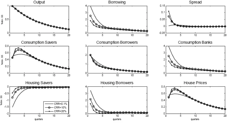
Figure 2 presents impulse responses to a technology shock for three di¤erent capital requirement
ratios. We observe that, when the capital requirement ratio increases, borrowing decreases, the interest
rate spread increases, and therefore borrowers consume less. Banks, since they are not able to lend as
much, also su¤er a decrease in their consumption. However, the e¤ect is the opposite for savers and this
compensates the e¤ect on borrowers and banks. Therefore, the overall e¤ects are distributional and they
do not a¤ect the aggregate. Notice that these are, though, …rst order level e¤ects and, while describing
the dynamics of the model, represent positive results. In order to infer some normative conclusion, a
welfare analysis must be made. We perform this exercise in the following section.
4
Welfare
4.1 Welfare Measure
To assess the normative implications of the di¤erent policies, we numerically evaluate the welfare derived
in each case. As discussed in Benigno and Woodford (2008), a popular approach that has recently been
Figure 2: Impulse responses to a technology shock. Di¤erent capital requirement ratios.
to the structural equations for given policy and then evaluating welfare using this solution. Thus, we
have used the software Dynare to obtain a solution for the equilibrium implied by a given policy by
solving a second-order approximation to the constraints, then evaluating welfare under the policy using
this approximate solution, as in Schmitt-Grohe and Uribe (2004).20 In particular, we evaluate the welfare
of the three types of agents separately. The individual welfare for savers, borrowers, and the …nancial
intermediary, respectively, is as follows:
Ws;t Et
1
X
m=0
m
s logCs;t+m+jlogHs;t+m
(Ns;t+m)
; (21)
Wb;t Et
1
X
m=0
m
b logCb;t+m+jlogHb;t+m
(Nb;t+m)
; (22)
Wf;t Et
1
X
m=0
m
f [logCf;t+m]: (23)
Following Mendicino and Pescatori (2007), we de…ne social welfare as a weighted sum of the individual
welfare for the di¤erent types of households:
2 0
Wt= (1 s)Ws;t+ (1 b)Wb;t+ (1 f)Wf;t: (24)
Each agent´s welfare is weighted by her discount factor; respectively, so that the all the groups receive
the same level of utility from a constant consumption stream.
4.2 Capital Requirement Ratios
Figure 3 displays the welfare that each group obtains when increasing the capital requirement ratio for
banks. Notice that results are presented in welfare units (utils),21 since the purpose of this …gure is
to illustrate the issue from an ordinal point of view.22 On the other hand, Table 3 presents a measure
for …nancial stability associated with di¤erent capital requirements. We take the standard deviation of
credit as a proxy for …nancial stability, since a stable …nancial system is one in which variability of credit
is low.
Remember that there are two distortions in this economy, corresponding to the two collateral
con-straints, the one for the borrowers and the one for the …nancial intermediaries, respectively. Capital
requirements a¤ect directly the second distortion. Savers do not su¤er from any of the distortions.23
We see that there is a welfare trade-o¤ between borrowers and savers. While savers are better o¤ when
banks are required to hold more capital, borrowers are initially worse o¤ with this measure. For the
range of values analyzed, savers are always better o¤ than in a situation with no regulation. Borrowers
are worse o¤ for initial increases but their welfare starts to recover for capital requirements greater than
6%. For capital requirements in the range of 6-16%, they are still worse o¤ than initially. Nevertheless,
for capital requirements larger than 16%, they are better o¤ than in a situation with no regulation. The
reason is that, initially, increasing the capital requirement does not allow borrowers borrow as much as
they would like, the interest rate spread increases, and therefore their consumption decreases. This is the
level e¤ect that a¤ects them negatively. However, as we can see in Table 3, a higher …nancial stability is
achieved the higher capital requirements are, and this fact has an e¤ect in terms of consumption stability.
For larger values of the capital requirement ratio, even though the level of consumption decreases, the
2 1"Utils" refer to the units of welfare in a utility scale. Therefore, the change in utils measures, from an ordinal point of
view, whether agents are better o¤.
2 2In this section and the next one, we do not consider welfare in consumption equivalent units since it is not clear what
the benchmark situation would be. However, in subsequent sections, when we make the comparison between Basel I, II with Basel III, we take the …rst case as a benchmark and present welfare gains from the new regulation in consumption equivalents.
2 3
volatility e¤ect prevails and this is why borrowers end up being better o¤. Saving is equal to borrowing
in equilibrium. Thus, since the level of borrowing decreases with higher capital requirements, savers can
use part of their saving for their own consumption. Therefore, savers are better o¤.
For banks, the argument is similar to the one of the borrowers. Albeit their welfare decreases for
lower values of the capital requirement ratio, it starts to increase from a certain value of this parameter.
When capital requirements increase, banks cannot lend as much as they would like and their constraint
becomes tighter. This negatively a¤ects their dividend as a level e¤ect. Nevertheless, welfare values
increase after a certain threshold of the capital requirement ratio. Thus, for lower values of the capital
requirement ratio, below the range of the Basel regulation, banks welfare slightly decreases. However,
increasing the capital requirement ratio further helps reducing the distortion implied by the collateral
constraint of bankers. Given that they cannot smooth their consumption by themselves, higher capital
requirements limit the loans they can make, stabilizing the …nancial system and, therefore, making their
pattern of consumption also more stable. This is the volatility e¤ect implied by a more stable …nancial
system, as shown in Table 3.
The lower left panel represents welfare of the households, disregarding banks. If we look at the
welfare of the households, we see that increasing capital requirements is welfare enhancing,24 that is, the
welfare gain experimented by the savers compensates the initial loss of the borrowers.25
Table 3: Volatility of Borrowing
CRR 1% 5% 10% 15% 20%
STD (B) 5:97 4:98 4:17 3:60 3:17
5
Optimal Implementation of Basel III
Basel III states that there should be an extra countercyclical capital bu¤er in order to avoid excessive
credit growth. The purpose of this bu¤er is the protection of the whole banking system from periods
of excessive credit growth activities. It will work on preventing banks from following more than needed
expansionary credit policies during economic booms that would increase the severity of in‡ation or more
than needed contractionary ones during de‡ation that would deepen the economic downturn.
The size of the bu¤er is set by the regulator and must take into account the macroeconomic
en-vironment in which banks operate. Therefore, it will be applied considering national circumstances of
2 4
Higher capital requirements increase borrower welfare in steady state. The e¤ects in transition may be di¤erent.
0 0.05 0.1 0.15 0.2 -50 0 50 100 150 Savers CRR Wel fare (ut ils )
0 0.05 0.1 0.15 0.2 -380 -360 -340 -320 -300 Borrowers CRR Wel fare (ut ils )
0 0.05 0.1 0.15 0.2 -2200 -2000 -1800 -1600 -1400 Banks CRR W elf ar e (ut ils )
[image:19.612.169.433.65.279.2]0 0.05 0.1 0.15 0.2 -7 -6.5 -6 -5.5 -5 Households CRR W elf ar e (ut ils )
Figure 3: Welfare derived from increasing the capital requirement ratio (in utils).
countries’banks and related …nancial institutions.
However, the Basel III accord does not fully specify the criteria to change the capital requirement or
under which speci…c conditions. There are, nevertheless, several things that we can infer from the Basel
III statement:
-The countercyclical bu¤er is a macroprudential policy that uses the capital requirement ratio as an
instrument.
-The main objective of this bu¤er in Basel III is to avoid excessive credit growth.
-The regulator should also use macroeconomic variables as indicators of excessive credit growth as
well as the credit growth itself.
Thus, along these lines, we propose a rule on the capital requirement ratio that includes credit growth,
house prices and output in order to explicitly promote …nancial stability. For the choice of the variables
to be considered in the rule, we have followed the guidance stated by the IMF, the Committee on the
Global Financial System, and the Basel Committee on Banking Supervision. The IMF (2013) states
that a rise in house price can act as a leading indicator of excessive credit growth since they lead to
wealth e¤ects that permit the increase in borrowing. This wealth e¤ect is present in our model through
the collateral constraint for borrowers. The Committee on the Global Financial System (2012) identi…es
real estate prices as a potential indicator that could guide the build-up of capital-based instruments.
and real estate prices in the stress tests that “can provide quantitative guidance on how capital levels
should be adjusted.”In turn, the Basel Committee on Banking Supervision, in its “Guidance for national
authorities operating the countercyclical capital bu¤er”(2010), recommends to consider credit variables
as well as a broad set of information to take bu¤er decisions in both the build-up and release phases.
Some examples of variables that may be useful indicators in both phases include various asset prices and
real GDP growth.
In this way, the countercyclical capital bu¤er would be implemented as a simple rule, in the spirit of
the Taylor rules used for monetary policy.26
CRRt= (CRRSS)
Bt
Bt 1
b Y
t
Y
y q
t
q q
(25)
This rule states that whenever regulators observe that credit is growing, or output and house prices
are above their steady-state value, they automatically increase the capital requirement ratio to avoid an
excess in credit. Then, this rule captures the macroprudential approach of Basel III so that it anticipates
credit growth and avoids it before hand, and it uses the capital requirement ratio as an instrument to
achieve this goal. The goal is explicitly embedded in the rule since capital requirements respond directly
to credit growth. This macroprudential rule also includes other macroeconomic variables that can be
seen as indicators of credit growth such as output and house price deviations from their respective steady
states.27
Then, we study what the optimal implementation of the macroprudential countercyclical capital
bu¤er would be, that is, the one that would maximize welfare.
5.1 Optimal Parameters
Table 4 presents the optimal parameters in equation (25) that maximize social welfare and compare
results in terms of welfare gains with respect to the benchmark (no regulation, that is, there is no capital
requirement).
We see that under Basel I and II (…rst column), only savers bene…t from higher capital requirements,
with respect to the no regulation situation. The second column shows the increase in capital requirements
2 6Note that the Taylor rule for monetary policy uses the interest rate as an instrument and it responds to output an
in‡ation.
2 7
stated in Basel III without taking into account the countercyclical capital bu¤er. We …nd that increasing
the capital requirements as in Basel III makes everyone better o¤ with respect to Basel I, II. Therefore,
Basel III, with no countercyclical bu¤er, already represents a welfare improvement with respect to Basel
I, II.
Albeit, optimally implementing the countercyclical capital bu¤er, that is the third column named
Basel IIIM P, manages to increase total welfare with respect to a situation of no regulation.
Never-theless, the losers in this case are the savers. Savers are better o¤ with increases in the static capital
requirement ratio but not with the countercyclical bu¤er, since it implies higher spreads. However, the
countercyclical bu¤er provides a more stable …nancial scenario, as it can be inferred from the volatility
of borrowing. Both borrowers and banks bene…t from this measure because it helps them both smooth
their consumption and reduce the collateral distortions that a¤ect them. Savers, who are not collateral
constrained, do not bene…t from this scenario.
In terms of the optimal implementation of the rule, we observe that the regulator should attach
relatively more weight to the output and the house price parameters in the rule, rather than to the
credit growth parameter. The reason is that these variables serve as an anticipated indicator of credit
growth and, therefore, help the regulator achieve its macroprudential goal; when the regulator observes
[image:21.612.133.478.438.736.2]credit growth itself, it may be too late to avoid it.
Table 4: Optimal Implementation of Basel III
Basel I, II Basel III Basel IIIM P
CRRSS 8% 8% + 2:5% 8% + 2:5%
b - - 0:1
y - - 1:9
q - - 1:6
Welfare gain
Savers 2:97 3:29 0:88
Borrowers 0:58 0:49 2:61
Banks 0:99 0:98 1:58
Total 0:99 0:96 4:61
Volatility of Borrowing
0 10 20 0 0.5 1 Output %d e v. S S
0 10 20
-5 0 5
Borrowing
0 10 20
-0.5 0 0.5
Spread
0 10 20
0 0.5 1 Consumption Savers %d e v. S S
0 10 20
0 2 4
Consumption Borrowers
0 10 20
0 2 4
Consumption Banks
0 10 20
-5 0 5 Housing Borrowers quarters %d e v. S S
0 10 20
0 0.5 1
House Prices
quarters
0 10 20
[image:22.612.173.455.67.280.2]0 2 4 Capital Requirement quarters Basel III Basel III MP
Figure 4: Impulse responses to a technology shock. Basel III versus Basel IIIM P.
5.2 Simulations
Here, we simulate the model for the Basel III requirements compared with Basel IIIM Pto study the
procyclicality of regulations, a much discussed topic in the literature. Basel III require a total capital of
10.5%. In order to simulate Basel IIIM P, we also consider a capital requirement of 10.5% in the steady
state, together with the optimal macroprudential rule found in the previous section for the capital bu¤er.
Notice, that this section is positive, describing the dynamics of the model. The previous section was
normative, studying welfare.
Figure 4 presents the model impulse responses to a technology shock for the two alternative scenarios:
Basel III and Basel IIIM P. Observe that these impulse responses are showing the pattern of the variables
following a shock, that is, their deviations from their steady state. Note that welfare calculations (Table
4) show second order approximations, that is, volatilities which can be used for normative evaluations.
Thus, Figure 4 and Table 4 are not directly comparable.
We see that under Basel IIIM P, following the technology shock, the capital requirement increases
about 2% with respect to its steady state, while it remains at the steady state under Basel III. This
higher capital requirement under Basel IIIM P makes borrowing not to increase as much with the shock.
Then, borrowers and banks can consume less under Basel IIIM P but this is compensated by an increase
in consumption by savers, which o¤sets aggregate di¤erences. In terms of procyclicality of the regulation,
the impact of this measure are countercyclical for the agents directly a¤ected by the capital requirement
ratio, i.e. borrowers and banks, while procyclical for savers.
6
Concluding Remarks
In this paper, we take as a baseline a dynamic stochastic general equilibrium (DSGE) model, which
features a housing market and a …nancial intermediary, in order to evaluate the welfare achieved by Basel
I, II, and III regulations. Therefore, in the model, there are three types of agents: savers, borrowers and
banks. Borrowers are constrained in the amount they can borrow. Banks are constrained in the amount
they can lend, that is, there is a capital requirement ratio for banks.
First, we evaluate how the model responds to changes in the capital requirement ratio from a positive
point of view. We observe that higher capital requirements decrease the quantity of borrowing in the
economy and, as a consequence, both borrowers and banks can consume less. This is o¤set by higher
consumption by savers.
Then, we calculate the welfare e¤ects of increasing the capital requirement ratio on the di¤erent
agents of the model. Our results show that there is a welfare trade-o¤ between borrowers and savers.
While savers are better o¤ when banks are required to hold more capital, borrowers and banks are
initially worse o¤ with this measure. On the one hand, increasing the capital requirement does not
allow them borrow and lend as much as they would like, respectively, and, therefore, their consumption
decreases. This is the level e¤ect that a¤ects them negatively. However, given binding constraints,
the …nancial system is more stable with higher capital requirements. For larger values of the capital
requirement ratio, this volatility e¤ect coming from a second-order approximation, which makes their
consumption more stable, prevails and both borrowers and banks end up being better o¤. For savers,
this implies a higher pattern of consumption because in equilibrium, when borrowing decreases, they do
not need to save as much.
After that, we propose a macroprudential rule for the capital bu¤er of Basel III (Basel IIIM P). With
this rule, capital requirements would respond to credit growth, output and house prices. We …nd the
optimal parameters of the rule that maximize welfare. The regulator should attach relatively more weight
to the output and the house price parameters in the rule, rather than to the credit growth parameter,
given that they serve as an anticipated indicator of credit growth. In terms of welfare, we see that the
no regulation.
Finally, using the optimized parameters, we simulate the model to study the procyclicality of Basel
IIIM P, a much discussed topic in the literature. We observe that, after a technology shock, capital
requirements increase under Basel IIIM P. This macroprudential rule cuts borrowing, achieving the goal
of the regulation, which is to avoid excessive credit growth. We add to the discussion …nding that Basel
IIIM P is countercyclical for borrowers and banks, the agents directly a¤ected by capital requirements,
Appendix
Steady-State of the main model
Cs+D=RsD+WsNs; (26)
Rs=
1
s
(27)
qHs
Cs
= j
(1 s)
(28)
Ws= (Ns) 1Cs (29)
Cb= s
1
s
B+WbNb; (30)
B = skqHb; (31)
b = ( s b); (32)
1
Cb
(q ( s b) skq bq) =
j
Hb
; (33)
Wb = (Nb) 1Cb; (34)
Cf +Bt= s
1
s
D+RbB; (35)
D
B = ; (36)
f = ( s f); (37)
1 ( s f)
f
Y =ANsNb1 ; (38)
Ws= A
Ns
Nb
1
; (39)
Wb =A(1 )
Ns
Nb
References
[1] Acharya, V. V. (2009), ‘A Theory of Systemic Risk and Design of Prudential Bank Regulation’,
Journal of Financial Stability, 5(3), pp. 224-255
[2] Admati, Anat R. and DeMarzo, Peter M. and Hellwig, Martin F. and P‡eiderer, Paul C., (2013).
“Fallacies, Irrelevant Facts, and Myths in the Discussion of Capital Regulation: Why Bank
Eq-uity is Not Socially Expensive. “Max Planck Institute for Research on Collective Goods 2013/23;
Rock Center for Corporate Governance at Stanford University Working Paper No. 161; Stanford
University Graduate School of Business Research Paper No. 13-7.
[3] Adrian, T., and A. Ashcraft (2012). “Shadow Banking: A review of the literature,” Unpublished
working paper, Federal Reserve Bank of New York State Report No. 580.
[4] Agénor, P., Pereira da Silva, L., (2011), Macroeconomic Stability, Financial Stability, and Monetary
Policy Rules, Ferdi Working Paper, 29
[5] Aikman, D, Haldane, A G and Nelson, B (2010), ‘Curbing the credit cycle’, available at
www.bankofengland.co.uk/publications/Documents/speeches/2010/speech463.pdf.
[6] Aikman, D, Nelson, B and Tanaka, M (2012), ‘Reputation, risk-taking and macroprudential policy’,
Bank of England Working Paper No. 462.
[7] Angelini, P., Neri, S., Panetta, F., (2011), Monetary and macroprudential policies, Bank of Italy
Working Paper
[8] Angeloni, I. and Faia, E. (2013). Capital regulation and monetary policy with fragile banks, Journal
of Monetary Economics, Vol. 60, Issue 3
[9] Bank of England (2009), ‘The Role of Macroprudential Policy’, A Discussion Paper
[10] Bank of England (2011), ‘Instruments of macroprudential policy’, A Discussion Paper
[11] Basel Committee on Banking Supervision, (2010), “Guidance for national authorities operating the
countercyclical capital bu¤er,” Bank for International Settlement publication
[12] Basel Committee on Banking Supervision, (2010), “The Basel Committee’s Response to the
[13] Benigno, P., Woodford, M., (2008), Linear-Quadratic Approximation of Optimal Policy Problems,
mimeo
[14] Bergin, P., Hyung-Cheol, S., Tchakarov, I., (2001), “Does exchange rate variability matter for
welfare? A quantitative investigation of stabilization policies,”European Economic Review, 51 (4),
1041–1058
[15] Bianchi, J (2011), ‘Overborrowing and systemic externalities in the business cycle’, American
Eco-nomic Review, Vol. 101, No. 7, pages 3,400–26.
[16] Borio, C. (2003). Towards a macroprudential framework for …nancial supervision and regulation?
BIS Working Paper No 128, February.
[17] Borio, C. (2011). Rediscovering the macroeconomic roots of …nancial stability policy: journey,
challenges and away forward. BIS Working Papers No 354, September.
[18] Brunnermeier, M., Crockett, A., Goodhart, C., Persaud, A. and Shin, H. (2009), ‘The Fundamental
Principles of Financial Regulation’, Geneva Report on the World Economy 11, ICBM, Geneva and
CEPR, London
[19] Clerc, L., Derviz, L., Mendicino C., Moyen S., Nikolov, K. Stracca, L., Suarez J., and Vardulakis,
A., (2014) "The 3D Model: a Framework to Assess Capital Regulation," Economic Bulletin and
Financial Stability Report Articles, Banco de Portugal, Economics and Research Department.
[20] Committee on the Global Financial System (2012), “Operationalising the selection and application
of macroprudential instruments,” CGFS Paper No 48
[21] Domeij, D., Flodén, M., (2006) "The Labor-Supply Elasticity and Borrowing Constraints: Why
Estimates are Biased." Review of Economic Dynamics, 9, 242-262
[22] Faia, E., Monacelli, T. (2007), “Optimal interest rate rules, asset prices, and credit frictions,”
Journal of Economic Dynamics and Control, 31 (10), 3228–3254
[23] Giese, Julia, Benjamin Nelson, Misa Tanaka and Nikola Tarashev (2013) How could macroprudential
policy a¤ect …nancial system resilience and credit? Lessons from the literature, Financial Stability
[24] Iacoviello, M. (2005), "House Prices, Borrowing Constraints and Monetary Policy in the Business
Cycle." American Economic Review, 95 (3), 739-764
[25] Iacoviello, M. (2015), "Financial Business Cycles", Review of Economic Dynamics, Vol. 18, Issue 1,
140-163
[26] Iacoviello, M. and Neri, S. (2010), “Housing Market Spillovers: Evidence from an Estimated DSGE
Model,” American Economic Journal: Macroeconomics, 2, 125–164.
[27] IMF, Monetary and Capital Markets Division, (2011), Macroprudential Policy: An Organizing
Framework, mimeo, IMF
[28] IMF, (2013). “Key Aspects of Macroprudential Policy: Background Paper,” IMF Working Paper
[29] Jiménez, G., Ongena, S., Peydro , J. and Saurina, J. (2014). “Macroprudential Policy,
Counter-cyclical Bank Capital Bu¤ers and Credit Supply: Evidence from the Spanish Dynamic Provisioning
Experiments.” European Banking Center Discussion Paper No. 2012-011.
[30] Kannan, P., Rabanal, P. and A. Scott, (2012): “Monetary and Macroprudential Policy Rules in a
Model with House Price Booms”, The B.E. Journal of Macroeconomics, Contributions, 12 (1)
[31] Kant, R. and Jain, S., (2013), "Critical assessment of capital bu¤ers under Basel III", Indian Journal
of Finance, Vol. 7, Issue 4
[32] Kim, J., Ruge-Murcia, F., (2009), “How much in‡ation is necessary to grease the wheels?,”Journal
of Monetary Economics, 56 (3), 365–377
[33] Lawrance, E., (1991), "Poverty and the Rate of Time Preference: Evidence from Panel Data", The
Journal of Political Economy, 99 (1), 54-77
[34] Longworth, D. (2011), ‘A Survey of Macro- prudential Policy Issues’, Mimeo, Carleton University
[35] Lorenzoni, G (2008), ‘Ine¢ cient credit booms’, Review of Economic Studies, Vol. 75, No, 3, pages
809–33.
[36] Mendicino, C., Pescatori, A., (2007), Credit Frictions, Housing Prices and Optimal Monetary Policy
[37] O¢ cial Journal of the European Union (14-02-2012). RECOMMENDATION OF THE EUROPEAN
SYSTEMIC RISK BOARD of 22 December 2011 on the macroprudential mandate of national
authorities
[38] O¢ cial Journal of the European Union, (15-06-2013). RECOMMENDATION OF THE
EURO-PEAN SYSTEMIC RISK BOARD of 4 April 2013 on intermediate objectives and instruments of
macroprudential policy
[39] Pintus, Patrick A. & Wen, Yi & Xing, Xiaochuan, 2015. "Interest Rate Dynamics, Variable-Rate
Loan Contracts, and the Business Cycle," Working Papers 2015-32, Federal Reserve Bank of St.
Louis.
[40] Repullo, R. and Suarez, J. (2013), "The procyclical e¤ects of bank capital regulation", Review of
Financial Studies,Vol. 26, Issue 2.
[41] Repullo, R. and Saurina, J. (2012). The Countercyclical Capital Bu¤er of Basel III: A Critical
Assessment. In the Crisis Aftermath: New Regulatory Paradigms. Edited by Mathias Dewatripont
and Xavier Freixas. Centre for Economic Policy Research (CEPR), London
[42] Rubio, M. (2011), Fixed- and Variable-Rate Mortgages, Business Cycles, and Monetary Policy,
Journal of Money, Credit and Banking, Vol. 43, Is. 4
[43] Rubio, M. (2014), Housing Market Heterogeneity in a Monetary Union. Journal of International
Money and Finance, Vol. 40.
[44] Rubio, M. and Carrasco-Galllego, J. (2014), "Macroprudential and Monetary Policies: Implications
for Financial Stability and Welfare", Journal of Banking and Finance, 49, 326–336
[45] Rubio, M. and Carrasco-Galllego, J. (2015), "Macroprudential and Monetary Policy Rules: A
Welfare Analysis", The Manchester School, Vol. 83, No. 2, 127–152
[46] Schmitt-Grohe, S. and Uribe, M. (2004), "Solving Dynamic General Equilibrium Models Using a
Second-Order Approximation to the Policy Function," Journal of Economic Dynamics and Control,