arXiv:1703.05768v1 [astro-ph.GA] 16 Mar 2017
Preprint typeset using LATEX style emulateapj v. 12/16/11
CANDELS MULTIWAVELENGTH CATALOGS: SOURCE IDENTIFICATION AND PHOTOMETRY IN THE CANDELS EXTENDED GROTH STRIP
Mauro Stefanon1,2, Haojing Yan2, Bahram Mobasher3, Guillermo Barro4,5, Jennifer L. Donley6, Adriano Fontana7, Shoubaneh Hemmati8, Anton M. Koekemoer9, BoMee Lee10, Seong-Kook Lee11, Hooshang Nayyeri3,12,
Michael Peth13, Janine Pforr14, Mara Salvato15, Tommy Wiklind16, Stijn Wuyts17, Matthew L. N. Ashby18, Marco Castellano7, Christopher J. Conselice19, Michael C. Cooper12, Asantha R. Cooray12, Timothy Dolch20,
Henry Ferguson9, Audrey Galametz7,15, Mauro Giavalisco10, Yicheng Guo4, Steven P. Willner18, Mark E. Dickinson21, Sandra M. Faber4, Giovanni G. Fazio18, Jonathan P. Gardner22, Eric Gawiser23, Andrea Grazian7,
Norman A. Grogin9, Dale Kocevski24, David C. Koo4, Kyoung-Soo Lee25, Ray A. Lucas9, Elizabeth J.
McGrath24, Kirpal Nandra15,26, Jeffrey A. Newman27, Arjen van der Wel28 Draft version March 20, 2017
ABSTRACT
We present a 0.4-8µm multi-wavelength photometric catalog in the Extended Groth Strip (EGS) field. This catalog is built on the Hubble Space Telescope (HST) WFC3 and ACS data from the Cosmic Assembly Near-infrared Deep Extragalactic Legacy Survey (CANDELS), and it incorporates the existingHST data from the All-wavelength Extended Groth strip International Survey (AEGIS) and the 3D-HST program. The catalog is based on detections in the F160W band reaching a depth of F160W=26.62 AB (90% completeness, point-sources). It includes the photometry for 41457 objects over an area of ≈206 arcmin2 in the following bands: HST ACS F606W and F814W;HST WFC3
F125W, F140W and F160W; CFHT/Megacamu∗, g′,r′,i′ andz′; CFHT/WIRCAMJ, H and K S;
Mayall/NEWFIRM J1, J2, J3, H1, H2, K; Spitzer IRAC 3.6µm, 4.5µm, 5.8µm and 8.0µm. We are also releasing value-added catalogs that provide robust photometric redshifts and stellar mass measurements. The catalogs are publicly available through the CANDELS repository.
Keywords: catalogs; galaxies: evolution; methods: data analysis; techniques: photometric
Email: [email protected]
1Leiden Observatory, Leiden University, NL-2300 RA Leiden, Netherlands
2Department of Physics and Astronomy, University of
Mis-souri, Columbia, MO 65211, USA
3Department of Physics and Astronomy, University of
Cali-fornia, Riverside, CA 92521, USA
4UCO/Lick Observatory, Department of Astronomy and
As-trophysics, University of California, Santa Cruz, CA 95064, USA 5Department of Astronomy, University of California at
Berke-ley, BerkeBerke-ley, CA 94720-3411, USA
6Los Alamos National Laboratory, Los Alamos, NM 87544
USA
7INAF - Osservatorio Astronomico di Roma, via Frascati 33, I-00040 Monte Porzio Catone (RM), Italy
8Infrared Processing and Analysis Center, California Institute of Technology, MS 100-22, Pasadena, CA 91125
9Space Telescope Science Institute, 3700 San Martin Drive, Baltimore, MD 21218, USA
10Department of Astronomy, University of Massachusetts, 710 North Plesant Street, Amherst, MA 01003, USA
11Center for the Exploration of the Origin of the Universe
(CEOU), Department of Physics and Astronomy, Seoul National University, Seoul, Korea
12Department of Physics and Astronomy, University of Cali-fornia, Irvine, CA 92697, USA
13Department of Physics and Astronomy, The Johns Hopkins University, 366 Bloomberg Center, Baltimore, MD 21218, USA
14Aix Marseille Universit´e, CNRS, LAM (Laboratoire d’Astrophysique de Marseille) UMR 7326, 13388, Marseille, France
15Max-Planck-Institut fur Extraterrestrische Physik, Giessen-bachstrasse 1, D-85748 Garching bei Munchen, Germany
16Department of Physics, Catholic University of America, Washington DC 20064.
17Department of Physics, University of Bath, Claverton Down, Bath, BA2 7AY, UK
18Harvard Smithsonian Center for Astrophysics, 60 Garden Street, MS-66, Cambridge, MA 02138-1516, USA
19School of Physics and Astronomy, University of
Notting-ham, NottingNotting-ham, UK
20Deptartment of Physics, Hillsdale College, 33 E. College St., Hillsdale, MI 49242, USA
21National Optical Astronomy Observatories, 950 N Cherry Avenue, Tucson, AZ 85719, USA
22NASA’s Goddard Space Flight Center, Greenbelt , MD 20771, USA
23Department of Physics and Astronomy, Rutgers, The State University of New Jersey, 136 Frelinghuysen Road, Piscataway, NJ 08854, USA
24Department of Physics and Astronomy, Colby College, Wa-terville, Maine 04901, USA
25Department of Physics, Purdue University, 525 Northwest-ern Avenue, West Lafayette, USA
26Astrophysics Group, Blackett Laboratory, Imperial College London, London SW7 2AZ, UK
27Department of Physics and Astronomy and PITT PACC, University of Pittsburgh, Pittsburgh, PA 15260, USA
1. INTRODUCTION
The Cosmic Assembly Near-infrared Deep Extra-galactic Legacy Survey (CANDELS; Grogin et al. 2011; Koekemoer et al. 2011) is a 902-orbit Hubble Space Telescope (HST) Multi-Cycle Treasury (MCT) program aimed at obtaining deep multi-wavelength photometric data for more than quarter million objects. Observa-tions followed a two-tiered strategy and were distributed over five fields.
The deeper layer of our survey (CANDELS Deep) covers ∼ 130 arcmin2 to a depth of 27.6−29.4 AB
(5σ limit for point sources) over the North and South fields of the Great Observatories Origins Deep Survey (Giavalisco et al. 2004). Its photometric depth has al-ready been shown capable of reaching 0.5L∗ galaxies at
z & 8 (see e.g., Finkelstein et al. 2015; Bouwens et al. 2015) and also to cover the low-mass end of the galaxy population at z ∼ 2 − 5 (e.g., Grazian et al. 2015; Duncan et al. 2014; Mortlock et al. 2015; Tomczak et al. 2014). The shallower layer of the survey (CANDELS Wide) extends the coverage to a total of∼720 arcmin2
down to a depth of 26.9−28.9 AB in five fields, namely GOODS-N, GOODS-S, the Extended Groth Strip (EGS; Davis et al. 2007), the Cosmic Evolution Survey field (COSMOS; Scoville et al. 2007), and the Ultra Deep Sur-vey field (UDS; Lawrence et al. 2007; Cirasuolo et al. 2007). Furthermore, the combination of photometric depth and covered area allow detection of potential luminous high-z galaxies, primary targets for follow-up observations with e.g., HST, Atacama Large Mil-limeter/submillimeter Array (ALMA) and James Webb Space Telescope (JWST) (see e.g., Yan et al. 2012; Oesch et al. 2015).
The multi-wavelength photometric catalogs for the GOODS-S and UDS fields have already been presented by Guo et al. (2013) and Galametz et al. (2013), re-spectively; photometric redshifts and stellar popula-tion parameters for these two fields are described by Dahlen et al. (2013) and Santini et al. (2015), respec-tively. The CANDELS GOODS-S data, combined to the medium bands from Subaru (Cardamone et al. 2010), were also used in Hsu et al. (2014) to compute pho-tometric redshifts of normal galaxies and AGN. The description of the multi-wavelength catalogs, photo-metric redshifts and stellar population parameters for the COSMOS and GOODS-N fields are presented by Nayyeri et al. (in prep.) and Barro et al. (in prep.), re-spectively. This paper presents the CANDELS multi-wavelength photometric catalog for the EGS field. Com-panion papers will present the rest-frame luminosities (Kocevski et al. 2016 in prep.) and the probability dis-tribution functions of photometric redshifts (Kodra et al. 2016 in prep.). Since the first observations (Rhodes et al. 2000, PI Groth 1994), the EGS has been the site of sev-eral surveys, notably the All-wavelength Extended Groth Strip International Survey (AEGIS, Davis et al. 2007) and the DEEP2+3 spectroscopic survey (Coil et al. 2004; Cooper et al. 2006; Newman et al. 2013; Cooper et al. 2011, 2012). The catalog is complemented by measure-ments of the photometric redshifts and stellar population parameters.
This paper is organised as follows. Section 2 describes the datasets used to construct our multi-wavelength
cat-alog. Section 3 discusses the World Coordinate Sys-tem (WCS) for the HST mosaics. Section 4 describes the procedures for the flux measurements over the wide wavelength range, while Section 5 presents the valida-tion tests of the multi-wavelength catalog. Secvalida-tion 6 presents the photometric redshift and stellar mass mea-surements. Our results are summarised in Section 7. Our catalogs are accessible on the primary CANDELS pages at MAST29, through the Vizier service30, and from the
CANDELS team project website31.
All magnitudes are given in the AB system. We adopted a standard cosmology with H0 = 70km s−1
Mpc−1, Ω
Λ= 0.7, Ωm= 0.3.
2. DATA
The CANDELS EGS field is centered at α(J2000) = 14h17m00s and δ(J2000) = +52◦30′00′′,
correspond-ing to high Galactic latitudes (b ∼ 60◦). The AEGIS
project provided deep HST ACS imaging data in the F606W and F814W bands to 5σdepths of 28.7 and 28.1 mag, respectively. The CANDELS survey adds deep
HST WFC3 F125W and F160W coverage, and increases the depth of the ACS F606W and F814W mosaics with new data from parallel observations (Grogin et al. 2011; Koekemoer et al. 2011).
The wavelength coverage is complemented by ex-tensive ground- and space-based imaging: UV data from GALEX (PI C. Martin); u∗, g′, r′, i, z′ from
CFHT/MegaCam observations; B, R, and I-band imag-ing obtained with the CFHT 12K mosaic camera (Cuillandre et al. 2001; Coil et al. 2004); near infrared (NIR) broad band J, H and KS imaging from the
WIRCam Deep Survey (WIRDS; Bielby et al. 2012); J and K-band data from the Palomar Observa-tory Wide-Field Infrared Survey (Conselice et al. 2008); medium-band NIR filters from the NEWFIRM cam-era (van Dokkum et al. 2009);HST WFC3 F140W data from the 3D-HST survey (PI van Dokkum; Skelton et al. 2014); IRAC maps from Spitzer SEDS (Ashby et al. 2013) and S-CANDELS (Ashby et al. 2015); MIPS data from FIDEL (PI: M. Dickinson); Herschel PACS 100µm and 160µm (Lutz et al. 2011) and HerMES SPIRE 250µm, 350µm, 500µm (Oliver et al. 2010) and 1.4 and 4.8 GHz VLA data (Willner et al. 2006; Ivison et al. 2007).
The field also benefits from substantial integration time (∼800ks) in X-ray by Chandra (Laird et al. 2009; Nandra et al. 2015)32. The area covered by the
CAN-DELS EGS footprint also has spectroscopic coverage from the DEEP2 survey (Coil et al. 2004; Cooper et al. 2006; Newman et al. 2013). Although spectroscopically incomplete, this survey provides redshift information for
∼ 5×10⁴ objects brighter than R < 24.1 AB
(corre-sponding to approximately z < 1.4), ∼ 1400 of which fall within the CANDELS EGS boundaries. The recently concluded DEEP3 survey (Cooper et al. 2011, 2012) in-creases the number of spectrscopic redshifts in the CAN-DELS EGS field to a total of∼2200. Furthermore, the 3D-HST project providesHST G141 slitless grism
spec-29https://archive.stsci.edu/prepds/candels 30http://vizier.u-strasbg.fr/viz-bin/VizieR 31http://candels.ucolick.org
Figure 1. Response curves of the 22 bands included in the CANDELS EGS multi-wavelength catalog normalized to a maximum value of unity. The response curves are organised over two vertically stacked panels for ease of presentation. The responses correspond to the filter transmission combined with the detector quantum efficiency as well as atmospheric transmission in the case of ground-based instruments.
troscopy over the F140W footprint.
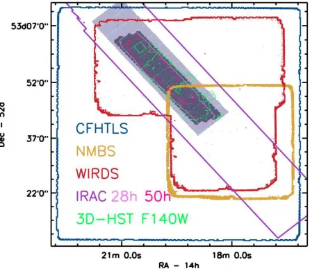
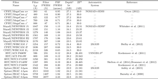
The multi-wavelength photometric catalog pre-sented in this work is assembled using data spanning from 0.4 to 8µm, taken by six different instruments. Specifically, the CANDELS EGS photometric cata-log is built using the data from CFHT/MegaCam, NEWFIRM/NMBS, CFHT/WIRCAM, HST/ACS, HST/WFC3 and Spitzer/IRAC. Figure 1 presents the response curves of the involved passbands, which are the convolution products of the filter transmissions and the detector throughputs. In case of the ground-based instruments, the atmospheric transmissions are also con-volved. Table 1 summarizes the main properties of each datatset. Similar to all the rest of the CANDELS fields (Guo et al. 2013; Galametz et al. 2013; Nayyeri et al. in prep.; Barro et al. in prep.), object detection was performed on the WFC3/F160W-band image. This mosaic is fully covered by all the adopted data sets, with the exception of the data from the NEWFIRM Medium-Band Survey (NMBS) and the WFC3 F140W mosaic which cover only about 1/3 and 2/3 of the F160W field respectively (see Figure 2).
2.1. HST
The HST data-set consists of both optical and NIR images, which were taken by the ACS/WFC and the WFC3/IR instruments, respectively. The WFC3 images were mostly obtained by the CANDELS program in Cy-cle 18 and 20. The ACS images consist of those obtained in the coordinated parallel mode during the CANDELS WFC3 observations and those from the AEGIS program obtained in Cycle 13 (Davis et al. 2007). A detailed description of HST data acquisition and reduction is presented by Grogin et al. (2011) and Koekemoer et al. (2011). We briefly summarize the main features below.
The AEGIS ACS data were taken in a mosaic pat-tern of contiguous tiles, covering an effective area of 10.′1×70.′5 in the F606W and the F814W bands. The
major axis of the rectangular area has a position angle of 40◦. The nominal exposure time was one orbit (∼2000
seconds) per filter.
The CANDELS WFC3 observations were performed
within the AEGIS ACS footprint, using a rectangular grid of 3 ×15 tiles and forming a contiguous field of 6.′7×30.′6 at a position angle of 42◦. Each tile was
ob-served in two epochs, separated by roughly 52 days and at different orientations (by 22◦). During each epoch a
given tile nominally received one orbit of observing time (∼2000 seconds)33. Each orbit was shared between the
F160W and the F125W filters such that ∼ 2/3 of the orbit was assigned to the former and ∼1/3 to the lat-ter, respectively. The observation in each filter within a given orbit was always divided into two sub-exposures. With the existing AEGIS ACS data in mind, the contem-poraneous CANDELS ACS parallel observations were taken in the F814W band during the first epoch and split evenly between the F606W and the F814W bands dur-ing the second epoch. As the ACS/WFC has a factor of 1.55×larger field of view than the WFC3/IR, the CAN-DELS ACS tiles overlapped heavily due to the abutting WFC3/IR tiling, and hence effectively resulted in 2-orbit and 1-orbit of exposures per pixel in F814W and F606W, respectively.
The WFC3 and ACS data were all reduced and combined following the approaches described by Koekemoer et al. (2011). The image mosaics used in this work have a scale of 60mas/pixel and all have the same world coordinate system. The WFC3 IR mosaics have nominal exposure times of ∼1300 and ∼2700 seconds in F125W and F160W, respectively. The ACS mosaics incorporate the contemporaneous CANDELS data and the earlier AEGIS data and have nominal exposure times of∼6000 and 12,000 seconds in F606W and F814W, re-spectively, reaching AB=28.8 and 28.2 mag (5σin aper-tures of 0.′′24 diameter, corresponding to 2× the
full-width-half-maximum (FWHM) of the point-spread func-tion (PSF)).
We also incorporated the WFC3 F140W images from the 3D-HST program (van Dokkum et al. 2011;
Figure 2. Coverage map of the different data sets used in this work. The dark filled area shows the coverage of theHST WFC3 F160W band from CANDELS, which has been adopted as the detection band. This area amounts to∼200 arcmin2. The light-blue filled region
reproduces the ACS F606W exposure map from the AEGIS project (Davis et al. 2007), which fully covers the F160W map. The other data sets are also outlined: CFHTLS (optical broad-bandu∗-to-z′, blue contour), WIRDS (Bielby et al. 2012; NIR J,H and Ks bands, red
contour), S-CANDELS (Ashby et al. 2015; dark purple: full coverage of the IRAC 3.6-to-8.0µm mosaics; pink: 28 hours depth; magenta: 50 hours depth coverages), NMBS (Whitaker et al. 2011; yellow contour), and 3D-HST (Skelton et al. 2014; green contour).
Brammer et al. 2012; Skelton et al. 2014). The 3D-HST survey was anHST Treasury program that offered spec-troscopic and photometric data in the CANDELS fields over a combined area of ∼ 625 arcmin2. 3D-HST
ob-tained imaging in the WFC3 F140W filter as well as spatially resolved spectroscopy with the WFC3 G141 grism. In the EGS field, the F140W imaging covered
∼ 2/3 of the CANDELS F160W footprint (see Figure 2) and reached average 5σ depth of 25.8 mag (in a 1′′
-diameter aperture). We used the v4.1 F140W mosaic produced by the 3D-HST team34, which has the same
WCS as the CANDELS WFC3 mosaics (see also Table 5 in Koekemoer et al. 2011).
2.2. Ground-based data
2.2.1. CFHTLS
The catalog incorporates flux measurements from the broad-bandu∗,g′, r′, i′, andz′ images obtained by the
34http://3dhst.research.yale.edu/Data.php
Megacam instrument at the 3.6m Canada-France-Hawaii Telescope (CFHT). These data correspond to the D3 field of the Deep component of the CFHT Legacy Sur-vey (CFHTLS); the field is 1 deg2in size and completely
covers the CANDELS EGS field.
For this work, we adopted the mosaics generated by the MegaPipe pipeline (Gwyn 2008) as described by Gwyn (2012). The sensitivity limits corresponding to the 50% completeness are u∗ = 27.5, g′ = 27.9, r′ = 27.6, i′ =
27.3, andz′ = 26.4 mag, for the five bands respectively
(Gwyn 2012). They were obtained by adding artificial point sources to the image after replacing the pixels of all the detected objects with a realisation of noise and recov-ering sources using SExtractor (Bertin & Arnouts 1996). The image quality is homogeneous across the bands, with the PSF FWHM average values of∼0.′′7−0.′′9.
The astrometric calibration was based on the Naval Observatory Merged Astrometric Dataset (NOMAD35),
and was refined using the Sloan Digital Sky Survey
Table 1
Summary of photometric data
Filter Filter Filter PSF Deptha ZPb Astrometric Reference
Name λeff FWHM FWHM 5σ System
(˚A) (˚A) (arcsec) (AB) (AB)
CFHT/MegaCamu∗ 383 61 0.95 27.1 30.0 NOMAD+SDSS Gwyn (2012)
CFHT/MegaCamg′ 489 144 0.90 27.3 30.0 ... ...
CFHT/MegaCamr′ 625 122 0.77 27.2 30.0 ... ...
CFHT/MegaCami′ 769 138 0.71 27.0 30.0 ... ...
CFHT/MegaCamz′ 888 87 0.71 26.1 30.0 ... ...
Mayall/NEWFIRM J1 1047 150 1.13 24.4 23.31 NOMAD+SDSSc Whitaker et al. (2011)
Mayall/NEWFIRM J2 1195 151 1.16 24.1 23.35 ... ...
Mayall/NEWFIRM J3 1279 140 1.08 24.0 23.37 ... ...
Mayall/NEWFIRM H1 1561 169 1.10 23.6 23.59 ... ...
Mayall/NEWFIRM H2 1707 176 1.06 23.6 23.61 ... ...
Mayall/NEWFIRM K 2170 307 1.08 23.5 23.85 ... ...
CFHT/WIRCAMJ 1254 157 0.72 24.4 30.0 2MASS Bielby et al. (2012)
CFHT/WIRCAMH 1636 287 0.68 24.5 30.0 ... ...
CFHT/WIRCAMKs 2159 326 0.65 24.3 30.0 ... ...
HST/ACS F606W 596 231 0.12 28.8 26.491 USNOB1.0d Koekemoer et al. (2011)
HST/ACS F814W 809 189 0.12 28.2 25.943 ... ...
HST/WFC3 F125W 1250 301 0.19 27.6 26.250 ... ...
HST/WFC3 F140W 1397 395 0.19 26.8 26.465 ... Skelton et al. (2014),Brammer et al. (2012)
HST/WFC3 F160W 1542 288 0.20 27.6 25.960 ... Koekemoer et al. (2011)
Spitzer/IRAC 3.6µm 3563 744 1.80 23.9 21.581 2MASS Ashby et al. (2015)
Spitzer/IRAC 4.5µm 4511 1010 1.82 24.2 21.581 ... ...
Spitzer/IRAC 5.8µm 5759 1407 1.94 22.5 21.581 ... Barmby et al. (2008)
Spitzer/IRAC 8.0µm 7959 2877 2.23 22.8 21.581 ... ...
Notes:
aThe 5σ-depths correspond to 5×the standard deviation of flux measurements in∼5000 circular apertures, with diameter of 2×FWHM
of the PSF, randomly placed across each image in the regions that are free of detected objects. bPhotometric zero-point.
cThe astrometric system was calibrated on the CFHTLS mosaics.
dThis is the original astrometric system adopted for calibration in Lotz et al. (2008). See Sect. 3 for further details.
(SDSS) DR7 catalog (Abazajian et al. 2009). The final internal and external astrometric uncertainties are 0.′′02
and 0.′′07, respectively (Gwyn 2012).
2.2.2. WIRCam Deep Survey
Deep broad-band J, H and Ks images from the WIRCam Deep Survey (WIRDS; Bielby et al. 2012) complement the HST WFC3 data. The images were obtained with the WIRCam instrument at the CFHT under good seeing conditions (FWHM∼ 0.′′6), and they
cover 0.4 square degrees centered on the EGS. The 50% completeness limit for point sources ranges be-tween 24.6-24.8 mag. The astrometry was calibrated us-ing the Two Micron All Sky Survey (2MASS) catalog (Skrutskie et al. 2006) with a final internal accuracy of
∼0.′′1 (Bielby et al. 2012).
2.2.3. NEWFIRM Medium Band Survey
The overlap of the CANDELS WFC3/F160W-band image with the mosaics of the NEWFIRM Medium Band Survey (NMBS, van Dokkum et al. 2009; Whitaker et al. 2011) amounts to ∼ 30% in the south-eastern region of the CANDELS footprint (see Figure 2). The CAN-DELS EGS multi-wavelength catalog incorporates these data. The data were taken with the NEWFIRM camera mounted on the Mayall 4m telescope at Kitt Peak. This NIR imaging survey used one traditional Ks filter and five medium-band filters in place of the usual J and H bands. Specifically, theJband was split into three filters J1,J2, andJ3, and theHband was split into two filters, H1 andH2 (van Dokkum et al. 2009; see also Figure 1).
The average seeing FWHM ranged between 1.′′06 to 1.′′16,
and the photometric depth reaches AB=23.5-24.4 mag (5σ in 2×FWHM apertures), with a 50% point-source completeness atKs=23.6 mag. The NMBS mosaics were aligned to the CFHTLSi′-band images with an
astromet-ric precision of∼0.′′1 over the entire field of view.
2.3. Spitzer
We also included the IR data from the Spitzer In-fraRed Array Camera (IRAC; Fazio et al. 2004), whose four bands center at 3.6, 4.5, 5.8, and 8.0µm.
The 3.6µm- and 4.5µm-band mosaics were obtained by combining four different image sets, two from the cryo-genic mission and two from the warm mission phases. The first cryogenic data imaged a narrow 2.3◦×0.29◦
strip overlapping with the AEGIS HST ACS imaging (PID 8, Barmby et al. 2008). The depth and width of the central ∼ 1◦ portion were later increased (PID
Nandra). All these IRAC data were reprocessed and mo-saicked using the same CANDELS HST tangent-plane projection and with a pixel scale of 0.′′6/pixels, to
pre-pare them appropriately for further photometric analy-sis (see also Ashby et al. 2015). The internal astrometry was checked by crossmatching approximately 500 point sources from the 2MASS catalog to the detections in the 3.6µm and 4.5µm mosaics. The 1σ dispersions in RA and Dec are.0.′′2 in both bands.
2.4. Value-added Data
The CANDELS EGS field has a large number of spec-troscopic redshifts and deep Chandra X-ray data. While they are not a part of the photometry, these data are included in our catalog (see Appendix A and C).
2.4.1. Spectroscopy
We included the spectroscopic redshifts from the DEEP2+3 Surveys (Coil et al. 2004; Willner et al. 2006; Cooper et al. 2011, 2012; Newman et al. 2013)36, which
were spectroscopic surveys targeting galaxies brighter than R=24.1 mag. Observations were carried out using the DEIMOS spectrograph on Keck 2 with a resolution of λ/∆λ∼5000 at the central wavelength of 7800˚A. In the EGS field, the campaign covered a∼30′×120′ strip
centered on the AEGIS ACS mosaic. Within the CAN-DELS F160W mosaic coverage, there are 2132 unique DEEP2+3 objects that have secure redshifts (quality pa-rameterQ≥3) within a matching radius of 0.′′8 (if more
than one object falls within the matching radius, the closest match was adopted).
2.4.2. X-ray data
The EGS field was initially observed by Chandra/ACIS with 200ks integration time as part of the AEGIS project (AEGIS-X Wide, Nandra et al. 2005; Laird et al. 2009). The observations covered the full AEGIS ACS mosaic with eight pointings, ∼17′×17′ each, for a total area
of ∼0.7 deg2. Recently, new Chandra/ACIS data to a nominal depth of 600ks were acquired over a region of approximately 0.29 deg2 centered on three central tiles
of the AEGIS-X Wide coverage. These data have been combined with the previous 200ks Chandra/ACIS obser-vations to provide a cumulative depth of 800ks in the three central ACIS fields (X Deep or AEGIS-XD, Nandra et al. 2015). The astrometry was cali-brated using the CFHTLS i-band image as the reference (Nandra et al. 2015). The AEGIS-XD is currently the third deepest X-ray survey in existence and it covers an area larger than the Chandra Deep Fields (CDFs) by a factor of 3. While being approximately 2−3 times shal-lower than the CDFs, it is sufficient to probe the dust-obscured X-ray galaxy populations at high redshifts (e.g., LX ∼1043 erg s−1at z ∼3 in the soft X-ray 0.5-2 keV
band).
3. ASTROMETRIC CALIBRATION OF CANDELSHST ACS AND WFC3 MOSAICS
The catalog is photometrically selected in WFC3 F160W band and hence it inherits the astrometry of
36 http://deep.ps.uci.edu/DR4/home.html and http://deep.ps.uci.edu/deep3/ for DEEP2 and DEEP3, re-spectively.
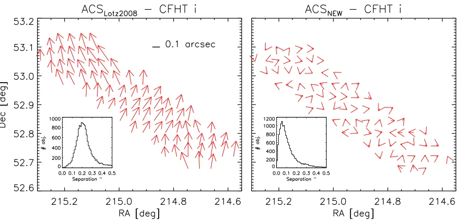
this image. The earlier astrometry of the CANDELS EGS WFC3 and ACS mosaics was calibrated using the AEGIS ACS catalog from Lotz et al. (2008). This cali-bration was based on the CFH12K mosaic of Coil et al. (2004), which was tied to the USNOB1.0 catalog. How-ever, a comparison between the F160W positions using this earlier astrometric solution and the CFHTLS D3 i′-band positions revealed systematic offsets. Figure 3
presents the measured offsets. Both the amplitude and the direction of the offset vary across the field, with a median offset of ∼0.′′2, significant enough to cause
po-tential problems in many applications. Indeed, previous works already showed that the median dispersion of the positions of a given object imaged on multiple overlap-ping plates in the USNOB1.0 catalog generated offsets up to 0.′′2−0.′′6 in the position of extended objects
com-pared to the SDSS Early Data Release (Stoughton et al. 2002 - see Monet et al. 2003 ) or to PPMX (Roeser et al. 2010).
Because the CFHTLS D3 astrometry implements higher-quality data and a better calibration (in partic-ular the SDSS calibration), we believe that it is more trustworthy. For the sake of internal consistency, we have opted to keep the WFC3 and ACS mosaic images unchanged in this version of the data release and to reg-ister all the F160W source positions to the CFHTLS D3 system at the catalog level.
This astrometric registration was achieved as follows. At first, we matched the WCS coordinates of the objects in the ACS F814W catalog of Lotz et al. (2008) to those in the CFHTLS D3 catalog of Gwyn (2012). A match-ing radius of 0.′′5 was adopted. The full region was then
divided into contiguous tiles, each 1.5×1.5 arcmin2 in
size. This size was chosen as a compromise between ob-taining a sufficient number (∼ 100) of objects in each tile to reduce the statistical uncertainties and yet keep-ing the tiles as small as possible in order not to lose the resolution. In each tile, the average of the displacements between the F814W and the CFHTLS coordinates was computed. These averages were used as the input to the
IRAF(Tody 1986, 1993) taskgeomapto generate the sur-face which converts one astrometric system to the other. The task was run interactively, adopting a 5th-order Leg-endre function to represent the surface, as it turned out to provide the best results in terms of residuals. In this process, we rejected a few objects with residuals larger than 3σ. Finally we re-registered the F814W coordinates to the new system by applying the best-fit surface to cor-rect the positions.
After applying the correction, the astrometry shows much less discrepancy with respect to the CFHTLS D3 system, with a median offset of∼0.′′04, i.e., a factor of 5×
Figure 3. Left panel: Offsets in RA and Dec positions between the previous CANDELS astrometric system (inherited from the AEGIS system) and the CFHTLS i-band system. Each arrow represents the average of the offsets measured from the matched objects within the rectangle region (1.′5×1.′5 in size) centered on the arrow tail.Right panel:Similar to the left panel, but after correcting the CANDELS
system to the CFHTLS system. The bands used for the recalibration are the ACS F814W and the CFHTLS i-band. In both panels, the insets show the distribution of the offsets (bin size 0′′.01): the median offset of the old astrometric calibration is 0.′′2, while that of the
[image:7.612.89.558.67.292.2]offsets after applying the new astrometric solution is 0′′.04.
Table 2
Main SExtractor parameters in the hot and cold mode
Parameter Name Cold Mode Hot Mode
DETECT MINAREA 5.0 10.0
DETECT THRESH 0.75 0.7
ANALYSIS THRESH 5.0 0.7
FILTER NAME tophat 9.0 9x9.conv gauss 4.0 7x7.conv
DEBLEND NTHRESH 16 64
DEBLEND MINCONT 0.0001 0.001
BACK SIZE 256 128
BACK FILTERSIZE 9 5
BACKPHOTO THICK 100 48.0
Lotz et al. (2008) and to the CFHTLS D3 system as well.
4. PHOTOMETRY
For the flux measurements in the CANDELS EGS pho-tometric catalog we adopted two different approaches, depending on the angular resolution of the images, as parameterised by the FWHM of the PSF charactersic of each band. For the high-resolution images, i.e., all the HST bands, the photometry was performed using
SExtractor(Bertin & Arnouts 1996) in dual-mode with a detection on the F160W band and measurements on the PSF-matched ACS/WFC3 images matched to the F160W resolution, the lowest in our HST dataset. For the low-resolution images, i.e., all the ground-based data and theSpitzer/IRAC images, the photometry was per-formed using the TFIT software (Laidler et al. 2007), which uses a morphological template fitting technique. These procedures have been extensively described by Galametz et al. (2013) and Guo et al. (2013).
4.1. PSF and convolution kernels
For the HST and IRAC bands, the empirical PSFs were constructed from a set of high S/N and isolated
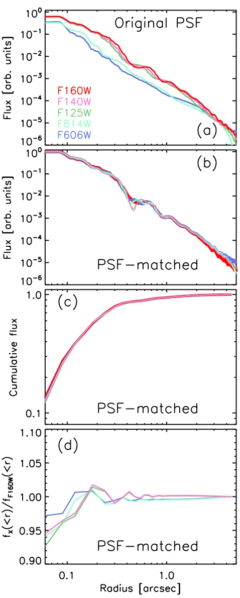
point sources using IRAF/DAOPHOT(Stetson 1987). De-spite the fact that IRAC PSFs vary across the mosaics due to the heterogenous nature of the input data and the intrinsic variations in the instrument itself, we opted for a single IRAC PSF in each band. For the ground-based optical and NIR images, the PSFs were created by stacking a number (6−21) of bright and isolated point sources. The convolution kernels were obtained using the IRAF/lucytask, for later uses in either PSF-matching orTFIT. Figure 4 shows the light profile of the empiricalHST PSFs before and after the PSF-matching process, together with the growth curves of the PSF-matched point sources. The growth curves do not show any significant offset with respect to that of the F160W band. Within the central 2 pixels (0.′′12), the differences
amount to ∼ 5%. By 8.3 pixels (0.′′5) the differences
essentially vanish.
4.2. Photometry of HST images
Both source detection and photometry were performed using a modified version of SExtractor v2.8.6, which was already used in the construction of the CANDELS UDS (Galametz et al. 2013) and GOODS-S (Guo et al. 2013) catalogs. This modified version provides a bet-ter measurement of the local background by imposing a minimum inner radius of 1′′ for the sky annulus (see
Grazian et al. 2006; Galametz et al. 2013) and refines the cleaning process by rejecting non-detections that are of-ten merged to real sources (Galametz et al. 2013).
CAN-Figure 4. Top to bottom panels: (a) Original PSF profiles of the
HST ACS F606W, ACS F814W, WFC3 F125W WFC3 F140W and WFC3 F160W bands. (b) Similar to the previous plot, but after PSF matching to F160W. (c) Growth curves in the same four bands after PSF matching. (d) Ratios of the cumulative flux in the four bands after the PSF-matching to that of F160W, shown as a function of radius. The color-coding scheme is the same in all panels.
[image:8.612.54.293.58.653.2]DELS GOODS-S and CANDELS UDS fields (Guo et al. 2013; Galametz et al. 2013). First,SExtractorwas run in the so-calledcold mode: the relaxed values of the de-tection parameters allow for a reliable extraction and deblending of the brighter sources. In the second run, called thehotmode, the detection parameters were tuned to optimize the detection of faint and blended objects. Table 2 presents the main Sextractor parameter values adopted for the cold and hot mode (see Appendix A in Galametz et al. 2013 for the full list of SExtractor pa-rameters). These two initial catalogs were then merged to keep the objects that are detected in at least one cat-alog. However, those objects in the hot catalog falling within the Kron (1980) ellipse of the cold-mode sources were rejected, as these are likely the result of an exces-sive source shredding (see also e.g. Caldwell et al. 2008, Gray et al. 2009, Barden et al. 2012).
The photometry in both the cold and the hot modes was performed in the dual-image mode of SExtractor, using the F160W band for the detection. As shown in Ta-ble 1, the FWHM ofHST PSFs differ from band to band, and the F160W-band PSF has the widest FWHM. To en-sure the most accurate color meaen-surements, we used the
IRAF/psfmatchtask to homogenize the PSFs of the mo-saics in the F606W, F814W, F125W, and F140W bands to the PSF of the F160W band. Figure 4 shows the pro-files of theHST PSFs before and after the PSF-matching procedure. The after-matching ones deviate from the F160W PSF at only a few percent level, which validates our matching process.
Different flux measurements were derived. Specifically, fluxes were measured using Kron (1980) elliptical aper-tures (SExtractor FLUX AUTO), isophotes (FLUX ISO) and a set of 11 circular apertures (FLUX APER). These individual values are reported in the supplemental cata-logs that accompany our main catalog.
The flux measurement provided by SExtractor in-side the Kron aperture is within 6% of the total flux (Bertin & Arnouts 1996), and it is thus often regarded as the measurement of total flux (but see e.g., Labb´e et al. 2003 and Graham & Driver 2005 for discussions on the deviation of SExtractorFLUX AUTOfrom the total flux). However, this often is not ideal for a faint source in terms of S/N because the large aperture needed to capture the total flux necessarily includes noise from many back-ground pixels, potentially swamping the signal from the targets. On the other hand, the isophotal flux that max-imizes the S/N for faint sources could underestimate the total flux because of the smaller aperture in use. If the flux measurements of a given object in different bands are done through the same aperture (i.e., through the dual-image mode as we did here), the isophotal fluxes will give the best measurements of colors. This kind of measurement is crucial for most of the possible applica-tions of our catalog such as SED fitting.
In our main catalog, the FLUX AUTO values were adopted as the total flux measurements in the F160W band. In any other HST bands, the quoted total fluxes were derived through the flux ratio with respect to the F160W band in terms of FLUX ISO, i.e.,
ftot,b=fiso,b×
fauto,F160W
fiso,F160W
Figure 5. Distributions of the pixel-by-pixel 1σmagnitude limits in the fiveHST bands in the EGS (blue solid line) and the UDS (grey dashed line) fields. The UDS catalog does not include the F140W band from 3D-HST. The limits were calculated from the RMS maps and are scaled to an area of 1 arcsec2. The bin width is 0.01 mag for all bands.
NMBS K IRAC 3.6um IRAC 4.5um WIRDS J
CFHT u
Figure 6. Examples of residuals after the second pass ofTFIT. Cutouts∼80′′×80′′from the original science images are shown in the top
row for CFHTu∗, WIRDSJ, NMBSK, IRAC 3.6µm and IRAC 4.5µm bands, respectively, from left to right. The corresponding cutouts
of the residual images are shown in the bottom row.
where ftot,b and fiso,b are the total and isophotal flux for band b, respectively, while fauto,F160W is the
Kron-aperture flux in the F160W band. The area adopted for the measurement of the isophotal flux fiso,b is de-fined from the F160W mosaic and it is thus the same for all bands. ftot,b is therefore a Kron-like flux measure-ment recovered from the higher S/N isophotal flux esti-mate. The validity of Equation 1 relies on the fact that the morphologies of the galaxies in our catalog do not vary with wavelength. Indeed, the majority of sources in our catalog have small sizes; furthermore, the smooth-ing introduced by the PSF-matchsmooth-ing to the F160W-band resolution further acts in the direction of homogeniz-ing the morphology of each source across the different bands. Similar approaches have been widely adopted in the literature (e.g. Whitaker et al. 2011; Guo et al. 2013; Galametz et al. 2013; Muzzin et al. 2013; Skelton et al. 2014). In particular van de Sande et al. (2013) showed that stellar masses from Whitaker et al. (2011) are con-sistent with dynamical mass measurements recovered from absorption lines, increasing the confidence on phys-ical parameter estimates from total flux measurements based on Eq. 1.
Figure 5 presents the distribution of the 1σ depth in eachHST band. The limiting magnitudes in the WFC3 bands roughly follow a tri-modal distribution, which is due to the different degrees of tile overlapping within the mosaics: the heavily overlapped regions among adjacent
tiles have higher sensitivities than what is typical, while the boundary regions of less coverage have lower sensi-tivities. The distribution for ACS limiting magnitudes is broader and more complex than that of the WFC3 ones. One possible explanation for this is that the ACS mo-saics are the result of two different datasets being com-bined together (AEGIS and CANDELS), each one likely with its own tri-modal distribution. Another possible explanation could be the different native pixel scale of the ACS camera compared to WFC3. The smaller pixel scale of ACS compared to WFC3 would result in lower S/N for each pixel (for the same cumulative S/N), intro-ducing the uncertainty. Overall, the depths correspond-ing to the peak of the distributions in 1σ magnitudes reported in Figure 5 for each band are generally within
≈0.1 mag from the rescaled 5σ depths presented in Ta-ble 1 (obtained from randomly placed circular apertures), supporting our rms maps generation. Finally, the plots show that the average depth of the EGSHST mosaics is slightly deeper than that of UDS.
4.3. Photometry of low resolution bands
4.3.1. TFIT flux measurement
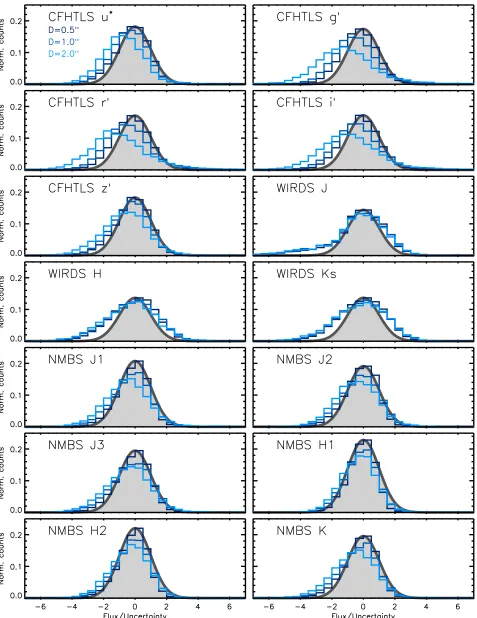
Figure 7. Histograms showing the background level in units of the local noise level, for the background-subtracted ground-based bands. The bin width is 0.5.The noise value was computed from the rms maps. The three different blue shades refer to empty apertures randomly positioned on the residual map avoiding any already detected source and adopting three different apertures: 0′′.5, 1′′. and 2.′′, as indicated by
the legend. These histograms have been renormalised to the total number of used apertures (∼104). For reference, we also plot as a grey
curve a standard normal distribution, whose peak value has been normalised to that of theD= 0′′.5 distribution. Most of the distributions
are centered on S/N∼0, and they are all consistent with zero at 3−σlevel, validating the background correction procedure. We relied
Papovich et al. (2001) and Laidler et al. (2007), while Lee et al. (2012) presented a set of simulations aimed at validating this template-fitting technique and quanti-fying its uncertainties. Briefly, the brightness profile of the source in the high-resolution image, identified from the segmentation maps, is convolved with the kernel quired to match the low-resolution image PSF. The re-sult is a template of the object in the low resolution im-age. Its total flux can then be obtained via best fit. In this way, it is possible to use all the information from the high-resolution image to deblend the objects in the low-resolution bands. This procedure assumes that the morphology of each object does not depend on the wave-length. A wavelength-dependent morphology could re-sult in the outer regions of some objects being excluded from their segmentation map. Furthermore, the out-skirts of fainter and/or smaller objects could fall below the detection threshold and hence be missing from the segmentation map generated during the detection stage. In order to limit the potential loss of flux due to these effects, the area associated with each object in the seg-mentation map was expanded following the empirical re-lation of Galametz et al. (2013). The fluxes measured byTFIThave been proven to be very close to total fluxes (Lee et al. 2012), and hence no further aperture correc-tion was applied to them.
Template fitting techniques require good alignment between the high-resolution and the low-resolution im-ages. However, the astrometric calibration of the low-resolution images could be different from that of the high-resolution one in the method and/or the reference catalog, which could result in slight offsets in alignment. Furthermore, geometric distortions, if not perfectly cor-rected, could also produce local misalignments among images. All this could result in catastrophic failures in template fitting. To overcome this problem, TFIT also measures small position offsets between the high and low resolution images. TFITis then run for a second time, using this information as part of the input to adjust the alignment locally by allowing a slight freedom of the cen-troid during the fitting process. Figure 6 presents an ex-ample of the second-pass residual images of a small sec-tion in the EGS field. The clean residual images indicate that the fitting procedure was successful.
4.3.2. Background assessment
A key factor in reliable flux measurement is the deter-mination of the background. TFITdoes not attempt any measurement of the background, but instead assumes a zero-background everywhere in the mosaic. Therefore, the background must be subtracted in advance. The full procedure of background estimate and subtraction for the CANDELS multi-wavelength catalog construction was described by Galametz et al. (2013).
We assessed the goodness of our background subtrac-tion by measuring the fluxes and the associated uncer-tainties in about 104 empty apertures (i.e., placed at
lo-cations free of known sources) across the residual images created by TFIT after subtracting off all the sources de-tected in F160W. The statistical distribution of the ratio between the flux measurements and their associated un-certainties should then be described by a standard nor-mal distribution (i.e. zero mean and unit standard de-viation). We performed the flux measurements adopting
three different aperture values (0.′′5, 1.′′0 and 2.′′0). Figure
7 shows the distribution of the S/N measurements for the ground-based data. The distributions very closely match the standard normal distribution, as expected.
Since the background subtraction in the IRAC bands is even more challenging, for these bands we complemented the above test with a Monte Carlo simulation as follows. A set of 500 positions were randomly chosen in regions free of any objects detected in the F160W band. We sim-ulated the presence of the objects by adding these 500 po-sitions to the input catalog for TFIT. As TFIT needs to refer to the segmentation map for the shape information, we also simulated exponential and de Vaucouleurs (1948) profiles through theIRAF mkobjecttask and added their footprints to the segmentation map. The science mosaics were not altered. The simulated objects have circularised effective radii uniformly distributed between 0.′′6 and 2.′′4
(after taking into account the PSF), which fully encom-pass the distribution of apparent sizes of the objects de-tected in the WFC3 F160W mosaic. TFITwas then re-run with this new catalog, adopting the same configura-tion used for the actual photometry, with the noise values computed from the rms maps. The forced flux measure-ments at the positions of the simulated sources, which are not actually present on the science mosaics, should statistically be zero.
The results from this test, in terms of S/N distribu-tion, are shown in Figure 8 together with the S/N from the empty aperture measurements. Most of the distribu-tions are centered on S/N∼0, and they are all consistent with zero at 3−σlevel, validating the background cor-rection procedure. We relied onSExtractorbackground measurement capabilities for theHST bands.
4.4. Multi-wavelength photometric catalog creation
Flux measurements from the PSF-matched bands and from the TFIT process were finally merged together to produce the final catalog. This step was trivial because each object kept its unique ID throughout all the pro-cesses, and therefore the matching was done based on the ID rather than on the coordinates.
The final catalog includes photometry in 22 bands for 41457 objects detected to a depth of 27.6 mag (5σ) in F160W. For each object, the catalog contains the flux measurement and the associated uncertainty. The cat-alog includes two distinct measurements for the IRAC 5.8µm and 8.0µm bands. One was obtained with an older kernel and was used for the computation of pho-tometric redshifts and stellar masses. The second mea-surement was obtained with an improved kernel (see Ap-pendix A). The plots presented in this paper refer to the improved kernel version of the IRAC 5.8µm and 8.0µm photometry. The catalog also includes all the objects with reliable (quality flag Q≥3) spectroscopic redshifts from DEEP2+3 (Coil et al. 2004; Newman et al. 2013; Cooper et al. 2011, 2012).
A flag mask, built from the F160W science mosaic, weight and rms maps, is included with the catalog in this data release to indicate if the object is very close to a bright star, falls within a defect region such as the
Figure 8. Histograms showing the background level in units of the local noise level, for the background-subtracted ground-based bands. The orange histograms present the data from the TFIT recovery of the simulated sources, while the blue, green and red ones refer to the apertures as indicated by the legend (see Sect. 4.3 for more details). These histograms have been renormalised to the total number of used apertures. The distributions are centered on zero, which further validate our background subtraction procedure.
Details on how the flag mask was generated are given in Appendix B of Galametz et al. (2013).
The EGS field is at Galactic latitude b ∼60◦;
there-fore the Galactic there-foreground extinction is expected to be minimal. Furthermore, the region of sky covered by the EGS footprint is small compared to the characteris-tic scale over which the Galaccharacteris-tic foreground extinction varies, hence a single value for the Galactic foreground extinction in each band for all the objects in the catalog should suffice. Considering also that the exact value of the extinction in each band depends on the adopted dust model (e.g., for EGSAV = 0.025 mag for a Cardelli et al. (1989) model orAV = 0.022 mag for a Fitzpatrick (1999) model) we opted not to apply any Galactic foreground extinction correction.
The main multi-wavelength photometric catalog is ac-companied by three additional catalogs containing esti-mates of the weight, based on the median exposure time inside the segmentation map, an estimate of the limit-ing magnitude, obtained from the median of the values in the rms maps from those pixels inside the segmen-tation map and a number of morphological and photo-metric quantities recovered from SExtractoron a per-object basis. We refer the reader to the README file for full details on the content of each of these catalogs. Together with the multi-wavelength photometric cata-log, with this work we also release the catalogs of pho-tometric redshifts, stellar masses and physical parame-ters for all the detected objects, derived following the procedures of Dahlen et al. (2013) and Mobasher et al. (2015). Appendixes A through D detail the content of each catalog. Two companion papers will present the rest-frame luminosities (Kocevski et al. 2016 in prep.) and the probability distribution functions of photometric redshifts (Kodra et al. 2016 in prep.).
For the CANDELS EGS multi-wavelength catalog, we also matched the positions of objects detected in the F160W mosaic to the objects detected in the Chandra 800ks maps of Nandra et al. (2015). The most reliable counterparts to the X-ray sources were identified using a maximum-likelihood technique using the redder and deeper bands available (see Nandra et al. 2015 for de-tails). The matching procedure resulted in 246 objects of the F160W-based-multi-wavelength catalog being likely X-ray emitters.
5. ASSESSMENT OF CATALOG PROPERTIES
In the following subsections we present the tests that we performed to check the consistency of the photom-etry. These tests consist of both comparisons to exter-nal catalogs and of the assessments of the interexter-nal self-consistency.
5.1. Detection completeness
The assessment of the completeness of sources in a cat-alog is a complex task, which ultimately depends on the class of objects considered and on the specific physical property under analysis. In this subsection we estimate the completeness in detection of sources, while in Section 6.4 we show an example of the completeness assessment in stellar mass.
We evaluated the detection completeness for both point and extended sources. For point sources, 100 PSFs randomly distributed across the whole field were added to the detection image without any restriction in their positions, and then we detected them using the same
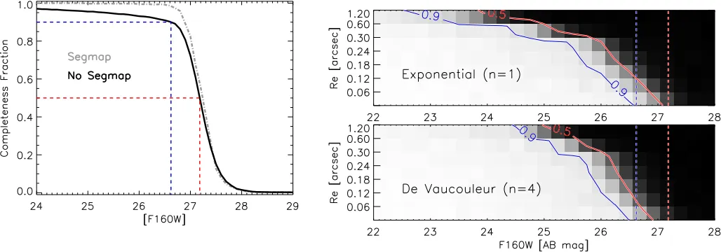
SExtractor configuration (two passes) adopted in the actual photometry. The process was repeated 20 times in each magnitude bin (width 0.25 mag) to increase the statistical significance. Although the above procedure provides robust completeness measurements for point sources, to allow for a more direct comparison with com-pleteness measurements from other surveys, the proce-dure was repeated excluding from the possible random positions those regions of the image which were already occupied by other sources, as identified by the segmen-tation map. This second method provides a strict up-per limit to the completeness measurement. The two curves are presented in the left panel of Figure 10. The curve corresponding to the detection completeness re-covered ignoring any restriction on object position (i.e. the no-segmap case) shows lower completeness values than those obtained excluding already detected sources (segmap case) for most of the magnitude range. This difference highlights the impact of source confusion. The 90% and 50% completeness limits for point sources are F160W=26.62 mag and 27.18 mag respectively, when the random positions are not checked against the segmenta-tion map. Excluding from the simulasegmenta-tion the posisegmenta-tion of all the detected objects, the limits are F160W=26.91 mag and 27.23 mag, respectively.
Figure 9. Left panel: Example of the mask adopted for brights stars and their spikes. The grey-scale image shows the cutout of the WFC3/F160W mosaic centered on a bright star arbitrarily picked from the photometric catalog. The yellow area marks the region set in the flag map to enclose the bright star and its spikes, as these could either contaminate the photometry and/or generate spurious detections.
Right panel: Example of teardrop. The figure shows the cutout of the rms map associated to the WFC3/F160W mosaic, centered on a region of higher rms signal (a teardrop, the white spot in the center). Regions like the one shown have also been detected and masked. The darker regions correspond to lower rms values from the overlap of contiguous exposures.
Figure 10. Detection completeness. The left panel shows the detection completeness on the CANDELS F160W image for a point-source, obtained from a Monte Carlo simulation. The dot-dashed grey curve is calculated masking all the already detected sources, while the solid black curve is calculated keeping all the sources. The blue and red dashed lines indicate the 90% and 50% completeness levels and corresponding magnitudes. The two panels on the right show the completeness for extended objects, for the two cases of an exponential (top panel) and a De Vaucouleur profile (bottom panel) with circularised effective radii in the range 0.′′06−1′′.2, obtained from a Monte
Carlo simulation. The solid red and blue curves mark the 50% and 90% completeness limits, while the vertical red and blue dashed lines represent the 50% and 90% completeness limits from the point source completeness simulation.
larger, which results in a lower S/N. This means that the S/N of extended objects falls below the detection thresh-old at a brighter total flux level as compared to that of point sources, resulting in a lower completeness for ex-tended sources. 2) Exex-tended objects are more prone to the source blending problem, and hence the difficulty to properly de-blend sources causes a further decrease of completeness.
In order to better model the effect of extended sources in the completeness estimate, the completeness for ex-tended sources was computed adopting two different
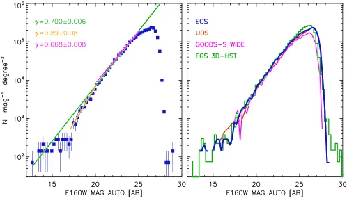
[image:13.612.46.560.366.546.2]posi-Figure 11. Left panel: Number counts based on the detection in WFC3 F160W band for CANDELS EGS (filled blue squares with poisson errorbars). The green, magenta and yellow lines represent the best-fitting power-law over the ranges 17 mag.F160W.25 mag, 17 mag
.F160W.20 mag, and 20 mag.F160W.25 mag, respectively. The measured power-law slopes are also indicated by the legend.Right panel: The CANDELS EGS number counts are compared to other measurements from the literature: CANDELS UDS (solid brown line), CANDELS GOODS-S (solid magenta line) and 3D-HST EGS (green histogram). The four measurements are barely distinguishable from each other for 19 mag.F160W.24 mag. The decrease in number counts starts at≈24.7 mag, while at F160W∼26.5 mag we observe an
abrupt decay in number counts, which is consistent with measurements from the other studies, and is likely a consequence of the detection image completeness for extended objects.
tion37, and photometry was performed with SExctractor.
The process was repeated ten times to increase the sta-tistical significance. The results are shown in the panels on the right side of Figure 10. The 90% completeness limits for the exponential and the de Vaucoulers profiles forRe= 0.′′3 (roughly corresponding to the median value
ofRe of the objects in the catalog with F160W brighter than 26.5 mag; theReof objects with magnitudes fainter than this value become close to those of point-sources) is 25.40 mag and 25.62 mag respectively.
As expected, the completeness limits for point sources reach fainter magnitudes than the corresponding limits for extended objects. Furthermore, objects with disky morphologies (n ∼ 1) and larger effective radii (Re & 0.′′3) tend to be missed by the detection algorithm at
brighter apparent magnitudes than objects with a more pronounced bulge (i.e.,n∼4). ForRe.0.′′3 the
detec-tion completeness curves on theRe−F160W plane, how-ever, roughly coincide. This is not unexpected, since less extended and/or more compact sources are less sensitive to the differences in the observed (i.e., PSF-convolved) light profile.
37 The uniform distribution of random positions still neglects the clustering of galaxies and thus provides an upper limit to the completeness. However, given the low number of added sources compared to the total number of objects in the catalog, the com-pleteness recovered in this way should still reflect a reliable estimate of the completeness for extended sources.
5.2. Number counts
The distribution of detected objects as a function of their apparent flux densities, the source number counts, is one of the most basic tests for the assessment of a sensitivity-limited catalog. The WFC3 F160W band number counts of our EGS catalog are presented in Fig-ure 11.
For magnitudes brighter than∼25 mag (which roughly corresponds to the completeness limit for our catalog when extended objects are taken into account), the num-ber counts can be fitted by a power-law with slope γ = 0.700±0.006. However, a better description of the data can be obtained by considering two power-laws: one in the range 17 mag.F160W.20 mag and a second for 20 mag .F160W.25 mag. In this case, the measured slopes areγ= 0.89±0.08 andγ= 0.668±0.008, for the brighter and fainter regimes, respectively. This double power-law behaviour is qualitatively consistent with dou-ble power-laws from previous analysis of number counts in NIR bands (see e.g., Gardner et al. 1993; Ashby et al. 2015).
[image:14.612.64.562.60.345.2]consis-tent with the EGS ones up to F160W∼26.5 mag. In the range 24 mag<F160W<26.5 mag the GOODS-S num-ber counts are below the UDS and EGS measurements by a factor up to 1.2 at F160W = 26 mag, which could be due to the slight shallower depth (0.2 mag) of GOODS-S compared to EGGOODS-S. The number counts from 3D-HGOODS-ST agree completely with the measurements from the CAN-DELS EGS catalog up to F160W ∼ 24 mag, while at 24 mag <F160W<26.5 mag they show an excess with respect to those from the CANDELS UDS and the CAN-DELS EGS up to a factor ∼1.2 at F160W ∼26 mag. One possible explanation for this excess could be that the detection for the 3D-HST catalog was performed on the noise-equalized combination of WFC3 F125W, F140W and F160W bands, which could help in the detection of fainter sources. At magnitudes fainter than F160W
∼26.5 mag we observe an abrupt decay in the number counts in all three catalogs, likely a consequence of the completeness for extended sources in the F160W band (adopted for the source detection).
5.3. Color-color plots
Figure 12 presents six color-color diagrams. We selected stars to be those objects with SExtractor CLASS STAR>0.9 and satisfying the following color-color criteria:
[z′−3.6µm]<0.73×[g′−z′]−1.8 for [g′−z′]≤1.5
(2) [z′
−3.6µm]<0.40×[g′ −z′]
−1.3 for [g′
−z′]>1.5
(3)
Most of the point sources occupy a well constrained region across the plots, which should correspond to the stellar locus. We compared the stellar locus to the syn-thetic colors of stars from stellar synthesis models. Fol-lowing what has been done for the CANDELS GOODS-S multi-wavelength catalog (Guo et al. 2013), and consid-ering that the stars in the EGS field should mainly be the halo population (due to its high latitude of b∼60◦)
and thus should be metal-poor, we adopted a set of stellar models of low metallicities ([M/H]=-0.5) from the BaSeL stellar synthesis models (Lejeune et al. 1997, 1998; Westera et al. 2002). All the plots show a good agreement between the observed colors of point sources with the colors from the synthetic library. Figure 13 shows a color-color diagram built with IRAC fluxes with S/N>5 in all four IRAC bands. The point sources (most of them are likely stars) have approximately zero color in the Vega system, consistent with models of stellar at-mospheres. The selection box, from Stern et al. (2005), identifies AGNs whose SEDs can be largely represented by a power-law (Donley et al. 2012); the X-ray sources constitute the majority of the objects inside the selec-tion box, supporting our color measurements. The X-ray sources outside the selection box are likely AGNs whose host galaxy outshines the active nucleus.
5.4. Comparison with publicly available catalogs
A number of multi-wavelength photometric catalogs have been produced in the EGS field, (Ilbert et al. 2006, Bundy et al. 2006, Whitaker et al. 2011, Barro et al. 2011a and Skelton et al. 2014). This Section compares the CANDELS multi-wavelength photometry to the
three publicly available catalogs that have a broad wave-length coverage and include the IRAC bands. Specif-ically, we consider the catalogs from the 3D-HST sur-vey (Skelton et al. 2014), the catalog from the NMBS (Whitaker et al. 2011), and the catalog presented by Barro et al. (2011a). The comparison is done on a per-filter basis. Figure 14 shows the comparison of the CAN-DELS EGS photometry to that directly available from the public catalogs. However, as we explain in Sect. 5.4.1, the total fluxes for the 3D-HST and NMBS cat-alogs were the result of a number of corrections (e.g, zero-point offsets, Galactic extinction, curve-of-growth). For this reason, Figure 15 presents a comparison after removing those corrections, as this should provide flux measurements as they were originally recovered from the mosaics.
5.4.1. 3D-HST
The 3D-HST multi-wavelength photometric catalog is described by Skelton et al. (2014). For the HST data, the measurements were done using SExtractor on the mosaics PSF-matched to the F160W band. The mea-surements for the ground based data and theSpitzerdata were done by using MOPHONGO (Labb´e et al. 2005, 2006, 2013), a procedure similar to TFIT but with the differ-ence that the photometry is done with a circular aperture after the target source is cleaned of its neighbours.
The measured fluxes of Skelton et al. (2014) were sub-ject to a number ofcorrections with the aim of providing accurate measurements of the total flux. Based on Labb´e et al. (2003; see e.g., their Figure 5) the SExtractor FLUX AUTO flux for faint sources can be systematically lower than the intrinsic total flux. Skelton et al. (2014) derived the offset between the two (i.e., the aperture cor-rection) from the growth curve constructed from bright point sources, and calculated the fraction of the light en-closed by the circular aperture that has the same area as the Kron ellipse used in determiningFLUX AUTO. The measurement of the total flux in the F160W band was then obtained by applying the corresponding aperture correction to the FLUX AUTO. As the size of the Kron ellipse depends on the flux and is smaller for a fainter source, the applied correction depended on the source brightness as well, and it was larger for a fainter source. Total fluxes for the other bands were recovered as
ftot,b=fap,b×
ftot,F160W
fap,F160W
whereftot,b andfap,bare the total and aperture flux for band b, respectively, while ftot,F160W is the total flux in
the F160W band. UV-to-K-band fluxes were corrected for the Galactic extinction following the extinction law of Cardelli et al. (1989; see Tab. 4 in Skelton et al. 2014). Finally, in Skelton et al. (2014) the photometric zeropoints were iteratively adjusted by computing the differences between the measured fluxes and the expected ones from the best-fit galaxy SEDs; the applied zeropoint offsets ranged from -0.22 mag in the u∗ band to +0.17
Figure 12. Color-color diagrams. Objects brighter than F160W= 26.5 mag in the EGS catalog are presented as a grey-scale density plot, with darker color marking denser regions. Objects brighter than F160W=22 mag and considered to be stars are marked by filled blue squares (see main text for details). The yellow stars mark the colors of the model stars based on the BaSeL library, which have [M/H]=-0.5 and are typical of the Galactic halo stars.
Figure 13. IRAC color-color plot. The blue points represent sources in the catalog with S/N>5 in all four IRAC bands, while the pink points mark objects withCLASS STAR>0.95 and F160W<
22 mag. The shaded region marks the AGN selection box defined by Stern et al. (2005); magenta open circles identify those objects with detection in the X-rays.
mag (e.g., HST/WFC3, WIRCAM/WIRDS) to ∼ 0.2 mag (e.g., CFHTu∗, NMBS J1 and IRAC 5.8µm).
How-ever, in most cases the difference between the two cata-logs is not a simple offset but has a dependence on the
flux, i.e., the difference increases at fainter magnitudes. The differences and their flux-dependent behavior likely stem from the various systematic corrections that the 3D-HST catalog has applied, namely, the total flux recovery on an object-by-object basis, the photometric zeropoint adjustments and the Galactic foreground ex-tinction corrections.
A comparison of colors is more straightforward in this context, as this largely (although still not com-pletely) circumvents the differences in the total flux re-covery. This comparison is shown in Figure 15, where we use the colors relative to F160W, i.e., we consider (mx−mF160W)CANDELS−(mx−mF160W)3D−HST, where
mx is the magnitude in band x. The colors based on
[image:16.612.35.274.437.616.2]Figure 15. Comparison of CANDELS EGS colors to the publicly available multi-wavelength catalogs from 3D-HST and NMBS. Zero-point offsets and Galactic extinction corrections have been removed from the 3D-HST and NMBS photometry. The plots present the quantity (mx−mref)CANDELS−(mx−mref)Otheras a function ofmx,CANDELS, wheremxis the magnitude in band x,mref is the magnitude in
The agreements in all bands are now much improved as compared to Figure 14, which supports our interpreta-tion meninterpreta-tioned above. Specifically, the∼0.2 mag offsets observed for some of the CFHT and NMBS bands have been largely reduced.
Considering that the flux comparisons done using the colors relative to the F160W band have the main effect of removing any dependence on aperture correction, the re-duced offset and the flattening of the color difference as a function of magnitude suggest that the offsets and trend observed in Figure 14 for these bands are likely the result of the corrections applied to the 3D-HST photometry to convert aperture into total fluxes. The agreement at the faint end is not as good as in the bright regime, which can be attributed to the smaller S/N for fainter sources and larger background flux. Nevertheless, all this sug-gests that the flux measurements in both catalogs have been performed in a self-consistent manner.
5.4.2. NMBS
The NMBS survey (Whitaker et al. 2011) was a medium-band NIR survey over the AEGIS and COSMOS fields. Source detection was performed on the K-band. Flux measurements for the optical and NIR images were performed by usingSExtractorin dual-image mode on the mosaics PSF-matched to the broadest PSF (i.e., the PSF of the H1 band). The K-band Kron (1980) fluxes were converted to total fluxes using a prescription similar to that adopted for the 3D-HST F160W total fluxes (see Whitaker et al. 2011 for details). The aperture fluxes for theSpitzer IRAC bands were measured using a pro-cedure very similar to that used for the 3D-HST photom-etry and converted to total flux using the ratio between the total and aperture flux in the K-band. The NIR medium-band filters pin-point the Balmer/4000˚A break at 1.5 .z .3, allowing for accurate photometric red-shifts measurements of objects in this range of redred-shifts. Because NMBS was carried out before the CANDELS project started, the multi-wavelength photometric cata-log does not includeHST/WFC3 data.
Figure 14 shows that the fluxes from both catalogs agree reasonably with each other, with the absolute dif-ferences generally being within ∼0.1 mag in the bright regime. Similar to the case for 3D-HST, the differ-ences show a flux-dependent trend, which is likely due to the systematic corrections applied in the NMBS cat-alog. Comparison of the difference in colors (Figure 15) shows much improved agreement in the sense that the flux-dependent behavior is largely removed. The ampli-tudes of the systematic offsets are similar to those found by the 3D-HST team (see e.g. Figure 34 of Skelton et al. 2014).
5.4.3. Barro+2011
The multi-wavelength photometric catalog of Barro et al. (2011a) was assembled by crossmatch-ing the SExtractor detections in IRAC 3.6µm and 4.5µm to the detections performed independently in each band, using a search radius of 2.′′0 Subaru R-band
imaging was used to reduce the multiple matches arising from the larger IRAC PSF. Photometry was carried out in each band using the Kron (1980) elliptical aperture obtained from the Subaru R-band mosaic. When
multiple counterparts to IRAC sources were found, IRAC fluxes were measured in 0.′′9 apertures after
deblending using a template fitting algorithm similar to that implemented in TFIT. Total magnitudes in the IRAC bands for such sources were finally calculated by applying the aperture corrections derived from the PSF growth curves.
The comparison between the CANDELS EGS photom-etry and that of Barro et al. (2011a) (Figure 14) shows a very good agreement for most of the bands, with offsets of .0.1 mag for the brighter sources. We do not show any color comparisons in Figure 15 corresponding to what we do in Section 5.4.1 and 5.4.2; indeed such a comparison would not have the advantages as in the previous two cases because no further corrections were applied to the
SExtractor flux automeasurements for all bands.
5.4.4. Summary
In this Section we compared the flux measurements in all bands from our catalog to the corresponding ones of the matching objects of three public cata-logs: Skelton et al. (2014), Whitaker et al. (2011) and Barro et al. (2011a). Since each team assembled their catalog using different tools and/or configurations and implemented different ways of measuringtotal fluxes, we considered two different approaches: 1) we compared the
total fluxes as directly provided by each team, and 2) we compared fluxes as closely as possible to those ini-tially recovered from the mosaics, removing any further correction that was successively applied (e.g., zero point adjustments, galactic extinction, aperture corrections). As such, comparisons in this second case should pro-vide a more reliable check on whether systematics in flux measurements exist between two different catalog. We presented the comparisons in Figure 14 and Figure 15, respectively.
Figure 14 shows that overall the flux measurements in our catalog systematically differ from those in the other three catalogs by up to ∼ 10%, with only few cases of systematic differences reaching∼20%. However, trends with magnitude are also present. These trends are almost totally absent when comparing to Barro et al. (2011a), while they are more visible when comparing to Skelton et al. (2014) and Whitaker et al. (2011). This flux-dependent behavior likely arise from the systematic corrections that were applied, namely, the total flux re-covery on an object-by-object basis, the photometric ze-ropoint adjustments and the Galactic extinction correc-tions.