Effect of structuring on coronal loop oscillations

(1)

Effect of Structuring on Coronal Loop

Oscillations

Michael Peter McEwan

Thesis submitted for the degree of Doctor of Philosophy

of the University of St Andrews

(2)

In this Thesis the theoretical understanding of oscillations in coronal structures is developed. In partic-ular, coronal loops are modelled as magnetic slabs of plasma. The effect of introducing inhomogeneities on the frequency of oscillation is studied. Current observations indicate the existence of magnetohydro-dynamic (MHD) modes in the corona, so there is room for improved modelling of these modes to under-stand the physical processes more completely. One application of the oscillations, on which this Thesis concentrates, is coronal seismology. Here, the improved theoretical models are applied to observed in-stances of coronal MHD waves with the aim of determining information regarding the medium in which these waves propagate.

In Chapter 2, the effect of gravity on the frequency of the longitudinal slow MHD mode is considered. A thin, vertical coronal slab of magnetised plasma, with gravity actingalongthe longitudinal axis of the slab is studied, and the effect on the frequency of oscillation for the uniform, stratified and structured cases is ad-dressed. In particular, an isothermal plasma, a two-layer plasma and a plasma with a linear temperature pro-file are studied. Here, a thin coronal loop, with its footpoints embedded in the chromosphere-photosphere is modelled, and the effects introduced by both gravity and the structuring of density at the footpoint layers are studied. In this case, gravity increases the frequency of oscillation and causes amplification of the ei-genfunctions by stratification. Furthermore, density enhancements at the footpoints cause a decrease in the oscillating frequency, and can inhibit wave propagation, depending on the parameter regime.

In Chapter 3, the effects introduced to the transverse fast MHD mode when gravity actsacrossa thin coronal slab of magnetised plasma are considered. This study concentrates on the modification of the frequency due to the dynamical effect of gravity in the equation of motion, neglecting the effect of strat-ification. Here, gravity causes a reduction of the oscillating frequency of the fundamental fast mode, and increases the lower cutoff frequency. In effect, for this configuration, gravity allows the transition between body and surface modes, in a slab geometry.

It is found, in these two studies, that each harmonic is affected in a unique manner due to structuring or stratification of density. With this knowledge, in Chapter 4, a new parameter is derived; P1/2P2, the

ratio of the period of the fundamental harmonic of oscillation to twice the period of its first harmonic. This parameter is shown to be a measure of the longitudinal structuring of density along a coronal loop, and the departure of this ratio from unity can yield information regarding the lengthscales of the structure. This process is highlighted using the known observations, indicating thatP1/2P2may prove to be a useful

diagnostic tool for coronal seismology.

(3)

Declaration

I, Michael Peter McEwan, hereby certify that this Thesis, which is approximately 60,000 words in length, has been written by me, that it is the record of work carried out by me and that it has not been submitted in any previous application for a higher degree.

Name:Michael P. McEwan Signature:...Date:...

I was admitted as a research student in October 2003 and as a candidate for the degree of Doctor of Philo-sophy in October 2004; the higher study for which this is a record was carried out in the University of St Andrews between 2003 and 2006.

Name:Michael P. McEwan Signature:...Date:...

I hereby certify that the candidate has fulfilled the conditions of the Resolution and Regulations appropriate for the degree of Doctor of Philosophy in the University of St Andrews and that the candidate is qualified to submit this Thesis in application for that degree.

Name:Bernard Roberts Signature:...Date:...

In submitting this Thesis to the University of St Andrews I understand that I am giving permission for it to be made available for use in accordance with the regulations of the University Library for the time being in force, subject to any copyright vested in the work not being affected thereby. I also understand that the title and abstract will be published, and that a copy of the work may be made and supplied to any bona fide library or research worker.

(4)

I would like to mention a few people who have contributed in various ways to this Thesis.

My supervisors over the past three years: I would like to thank Bernie for his guidance and encouragement over the course of my degree. You have allowed me the freedom to work with others throughout my degree, and as such, have helped create a Thesis of which I am proud. I would like to mention your red pen; you have read draft after draft of this Thesis, and helped me to compose it, and I am very grateful for all the time and effort you have given me over the past few years. I thank Ineke for many useful discussions, for supervising the work presented in Chapter 5 and for taking the time to read various drafts of my work. I also thank Toni for your excitement about science and your supervision in the production of Chapter 3, and many other sections in this Thesis (also for the notes in Spanish that I managed to translate!).

I express my gratitude to PPARC for the financial support they have provided for the past three years.

My friends, from all places, you have kept me going on many occasions, and have inspired me when you are successful. In particular, I would like to mention the guys from football: Will, Steve, Toni and the rest, even the silly chats we have can yield ‘some’ useful advice! From Jentris: Barry, Dom, Tom, Grant and the others, for being my close friends over the past few years, providing support when it is needed, and all those good stories on a Friday! Toallof my officemates, but in particular Paul, Alexandra and Dee who have had ‘the long haul’, all of you have provided a friendly and fun environment to work in, and I have enjoyed sharing a room with all of you.

Finally, my family: Mum; Dad; Alistair; Lesley and your clan. Lesley, the support you, Eugene, Andrew, Se´an and Ciara have provided over the last few years is invaluable to me. Alistair, you beat me, congratula-tions on your Thesis but more importantly, congratulacongratula-tions to you and Kate on your new family with Calum and James! Your advice over the years has kept me going on many occasions.

(5)

1.5 (a) Typical example of a flaring coronal loop (TRACE, 1999), observed using TRACE. Flaring loops are highly dynamical and are often observed to rise out of a flare site, with plasma draining down to the footpoints as the plasma cools. (b) MDI magnetogram of the solar disk (SOHO, 2005), black areas are regions of positive magnetic flux and white areas are negative flux. . . 5

1.6 Polar diagram of the phase speedcph=ω/kof the magnetoacoustic waves and the Alfv´en

wave. The phase speedcphis a function of the angleθbetween the wave vectorkand the

unperturbed magnetic field, B0(aligned parallel to the horizontal axis). (a)cA > cs, (b)

cs> cA. . . 15

1.7 Sketch of the spatial structure of the surface and body waves in either a slabora cylin-der. Here both the symmetric (sausage) modes and the antisymmetric (kink) modes (after Roberts (1985)) are shown. . . 22

1.8 Dispersion diagram for the phase speedcph = ω/k of the magnetoacoustic waves in a

coronal flux tube of radius a(after Edwin and Roberts 1983). The dispersive fast kink

mode is shown, propagating at speedck, a speed which varies askaincreases. Also the

slow sausage mode is shown, cT; which is only very weakly dispersive. In this diagram

cAe= 2cAiandci= 0.2cAiwithce= 0.1cAi. The solid lines represent the anti-symmetric

kink modes and the dashed lines represent the symmetric sausage modes. . . 24

2.1 Cartoon of a coronal loop of internal radius aand height h. The vertical z-axis points

upwards, opposite to gravity (with gravitational acceleration g). The vertical dashed line indicates the axis of symmetry. . . 27

(9)

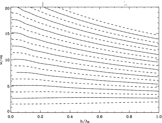
2.2 Dispersion diagram for the standing acoustic modes in an isothermal atmosphere. Hereω

is the frequency of the acoustic mode, measured in units of the coronal cutoff frequency

Ω = Ω0 = Ωc, andL/Λ0 is the dimensionless half-length of the loop in units of the

pressure scale heightΛ0. The dashed curves are the odd modes given by Eq. (2.78) and the

solid curves are the even modes given by Eq. (2.76). . . 37 2.3 First four eigenfunctions ofvz(z, t= 0). The loop apex is atz= 0and the loop footpoint

here is atz/Λ0= 5. Here,cs= 150km s−1andg= 274m s−2. . . 37

2.4 The solid line indicates the period of theω1mode (the even mode withn= 1), measured

in units of the acoustic cutoff periodPg= 2π/Ω, varying with increasing loop half-length,

L/Λ0 in a stratified atmosphere (given by Eq. (2.81)). Here,cs = 150km s−1andg =

274 m s−2. The dashed line indicates the equivalent dimensionless period in a uniform

atmosphere for whichg= 0andΩ = 0(given by Eq. (2.80)). . . 38

2.5 The two layer model for a straightened coronal loop, with a lower dense and cool chromo-spheric layer. The coronal part of the loop is of total extent2L, below which is a

chromo-spheric base of extenth. The total loop length is2(L+h). . . 39

2.6 Dispersion curves comparing the modes of oscillation of the two layer model (withh = 0.001L) and the modes of the isothermal model. The modes of the two layer model are

given by the solid curves and the modes of the isothermal single layer model are shown by the dashed curves. HereΛ0= Λc,Ω0= ΩcandΩch= 10 Ωc. . . 44

2.7 Dispersion curves as a function ofL/Λ0for the two layer model withΛc/Λch= 10(so the

dimensionless cutoff frequencyΩchin the chromosphere is 10 Ωc), whenh/Λc = 0.1L.

The solid curves are the modes of oscillation in the two layer model and the dashed curves are the modes of the single layer model. In the diagramΛ0= ΛcandΩ0= Ωc. . . 44

2.8 As in Fig. 2.7 but withh/Λc= 0.25L. . . 45

2.9 Diagram showing the effect of varying the dimensionless chromospheric extent,h/L, for a

fixed value ofL/Λc= 2.5. (HereΛ0= Λc). . . 45

2.10 Diagram highlighting how ∆ω/ω = (ωh−ωh=0)/ωh=0 varies with varying footpoint

extenth/L. Here the solid line represents the variation in frequency of the first odd mode

and the dashed line represents the first even mode.L/Λc = 2.5in this diagram. . . 46

2.11 Global eigenfunctionsvz=v(z)eiωtfor the two finite isothermal layers, simulating a dense

chromosphere. Herecs = 150km s−1,cch = 15km s−1andh = 0.1L. The loop apex

is atz = 0and the loop footpoint is atz/Λ0 = 5.5. The solid vertical line atz/Λ0 = 5

indicates the extent of the chromosphere (fromz/Λ0= 5toz/Λ0= 5.5). . . 46

2.12 Dispersion diagram for the two layer model withh = 0.1L, allowing for an evanescent

lower layer. The solid curves indicate the real frequencies for the even and odd modes and the dashed curves indicate the imaginary frequencies. Again the upper dot-dashed line indicates the chromospheric cutoff,Ωch = 10 Ω0(withΩ0= Ωc). . . 48

2.13 As in Fig. 2.11 but with wave leakage allowed for. Notice the wave motion is evanescent in the chromospheric region. . . 48

(10)

are the numerical solution of the dispersion relations (2.106) and (2.107) and the dashed curves are the approximate solutions given by Eqs. (2.122) and (2.123). . . 51 2.15 Dispersion diagram for the two layer model, with an infinite lower layer. The solid curves

indicate the propagating modes, or the real frequencies, and the dashed curves indicate the evanescent frequencies. Again the upper dot-dashed line indicates the solar interior cutoff term,Ωch= 10 Ω0(withΩ0= Ωc). . . 53

2.16 As in Fig. 2.13, but with an infinite depth of chromosphere (interior) plasma. . . 53 2.17 Time-space diagram for the simulation withcs= 7.5km s−1,θ= 40degrees andPdrive=

300s. The wave decays before reaching the far side of the box. . . 55

2.18 Time-space diagram for the simulation withcs= 7.5km s−1,θ= 50degrees andPdrive=

300s. Here, the wave propagates to the far side of the box. . . 55

2.19 Diagram comparing the frequencies satisfying Eqs. (2.153) and (2.155) for the linear tem-perature gradient model, withλ→1, to the frequencies given by the isothermal single layer

dispersion relations for the odd and even modes with frequencies given by Eqs. (2.76) and (2.78. The solid curves are the modes for the temperature gradient model and the dashed curves represent the isothermal model. HereΛ0= ΛapexandΩ0= Ωapex. . . 60

2.20 Dispersion diagram for the frequencies of the standing acoustic modes, as a function of

L/Λ0, in a coronal loop with a linear temperature gradient. The loop apex is 10times

hotter than the base (λ= 10). HereΛ0= ΛapexandΩ0= Ωapex. . . 61

2.21 Dispersion diagram as a function ofλ(ratio of apex temperature to base temperature) with L/Λ0= 2.5. The solid curves represent the odd modes and the dashed curves are the even

modes. . . 61 2.22 An illustration of the structure of the two layer model for a straightened coronal loop. The

blue section (transition region) has a linearly increasing temperature, fromTbasetoTapex

and the isothermal region has constant temperatureTapex. The coronal part of the loop is

of total extent2cL, the transition region extent ismLat either end. The total loop length is

2L(m+c), wherem+c= 1. . . 62

2.23 Diagram comparing the dimensionless solutions, given by the solid curves, of the transition region dispersion relations, Eqs. (2.163) and (2.165), in the limit ofm → 0- modelling

a fully isothermal corona, with frequencies given by Eqs. (2.76) and (2.78), given by the dashed curves (here, directly under the solid curves). . . 64 2.24 Diagram comparing the dimensionless solutions, given by the solid curves, of the transition

region dispersion relations, Eqs. (2.163) and (2.165), in the limit ofc → 0- modelling a

loop increasing in temperature linearly from the base atz =Lto the apex atz = 0, with

capex/cbase = 10. The frequencies given by Eqs. (2.153) and (2.155) are denoted by the

dashed curves (again, directly under the solid curves). . . 64 2.25 Diagram showing the effect of increasing the transition region extenth=mLfor a fixed

ratio ofcapex/cbase. Here,(m+c)L/Λc = 2.5andλ= 5. The solid curves represent the

odd modes and the dashed curves are the even modes. . . 66

(11)

2.26 Diagram showing the effect of increasing the ratio ofλ=capex/cbasefor a fixed extent of

transition region. Here,c= 0.8andm= 0.2with(m+c)L/Λc = 2.5. The solid curves

represent the odd modes and the dashed curves are the even modes. . . 66

3.1 Sketch of a coronal loop of heighthand width2a, in the presence of gravityg. . . 70

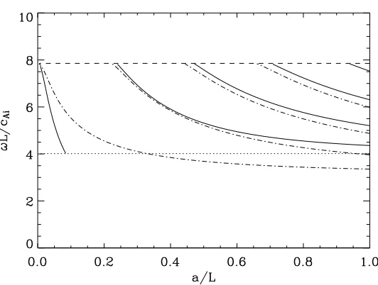
3.2 Horizontal coronal loop model with gravity acting perpendicular to the magnetic field. . . 71 3.3 Dispersion diagram showing the solution to Eq. (3.85) under the assumption of symmetric

and antisymmetric modes. As gravity is neglected in this derivation the assumption is valid. The solid lines are for the antisymmetric modes and the dotted lines represent the symmetric modes. HerecAi/cAe = 2/5. The dot-dashed line and the dotted line represent the upper

and lower cutoff frequencies, respectively. . . 85 3.4 Dispersion diagram showing the solution to Eq. (3.84) for body modes in the corona. Here

there is no longer any assumption of symmetric or antisymmetric modes. Parameters as in Fig. 3.3. The dot-dashed line and the dotted line represent the upper and lower cutoff frequencies, respectively. . . 85 3.5 Sketch showing the spatial difference between surface and body modes in a slab of plasma

(after Roberts (1985)). . . 86 3.6 Dispersion relation (3.60) for the first three surface modes (n= 1,2,3) for the caseg= 0

in a slab of half lengthL/Λc = 2.5. The solid lines indicate that the dispersion relation

is never zero (confirmed numerically), and therefore has no solution. Hence there are no surface modes in the corona. HerevAi=cAi. The vertical dashed lines indicate the values

of the upper cutoff, in the absence of gravity, forn= 1,2and3, respectively. . . 88

3.7 (a) Dispersion relation (3.60) for a slab of dimensionless half-lengthL/Λc = 2.5for the

three casesgL/2c2

Ai = 0(the solid line),gL/2c2Ai= 4(the dotted line) andgL/2c2Ai= 10

(the dot-dashed line). The vertical dashed line represents the zero gravity cutoff. Notice that the cutoff is modified with increasing gravity. . . 88 3.8 Dispersion diagram for the fast body mode solutionωL/cAi(solid curves) to Eq. (3.71) as

a function ofa/L. Here,gL/2c2

Ai= 1andcAi/cAe= 2/5. The dot-dashed curves indicate

the equivalent diagram with g = 0. The dashed and dotted lines indicate the upper and

lower cutoff frequencies, respectively. . . 90 3.9 Dispersion diagram for the fast body mode solutionsωL/cAi (solid curves) to Eq. (3.71).

HeregL/2c2

Ai= 2.5andcAi/cAe= 2/5. The dot-dashed line indicates the equivalent

dia-gram withg= 0, the dashed and dotted lines indicate the upper and lower cutoff

frequen-cies, respectively. Notice that the fundamental kink mode falls below the cutoff frequency, becoming a modified body mode. . . 90 3.10 Dispersion diagram for the fast body mode (solid curve) of oscillation in a uniform coronal

slab given by Eq. (3.71). The dashed and dotted lines indicate the upper and lower cutoff frequencies, respectively. Here,g= 0anda/L= 0.1. . . 91

3.11 Dispersion diagram for the fast body mode (solid curve) of oscillation in a horizontal coronal slab given by Eq. (3.71). The dashed and dotted lines indicate the upper and lower cutoff frequencies, respectively. Here,gL/2c2

Ai = 1.5anda/L= 0.1. . . 91

(12)

and lower cutoff frequencies, respectively. Here,gL/2c2

Ai= 2.5anda/L= 0.1. . . 92

3.13 Dispersion diagram for the fast body mode solutionωL/cAi(solid curve) to Eq. (3.71) as

a function ofgL/2c2

Ai. The dashed and dotted lines indicate the upper and lower cutoff

frequencies, respectively. Here,a/L= 0.1andcAi/cAe= 2/5. . . 93

3.14 Dispersion diagram for the fast body mode solutionsωL/cAi(solid curves) to Eq. (3.71)

as a function ofgL/2c2

Ai. The dashed and dotted lines indicate the upper and lower cutoff

frequencies, respectively. Here,a/L= 1.0andcAi/cAe= 2/5. . . 93

3.15 Sketch of thevxcomponent of the Alfv´en mode. Notice that there are no trapped solutions

forvx6= 0. . . 96

3.16 Coronal loop model: gravity aligned with the magnetic field. The slab is symmetric about the horizontal dashed line atz= 0for stability. . . 97

4.1 The dispersion diagram for magnetoacoustic waves in a magnetic flux tube of radius a.

The diagram gives the phase speedcph(=ω/k)of the modes as a function of longitudinal

wavenumberk(in dimensionless units ofka). The solid curves give the fast kink modes,

the dashed curves are the fast sausage modes. Also shown is the weakly dispersive band of slow waves (sausage and kink) with speed close tocT i, the slow mode speed in the tube

interior. Here the internal Alfv´en speedcAiis half the Alfv´en speedcAein the environment,

ci= 0.2cAiandce= 0.1cAi. (After Edwin and Roberts (1983)). . . 105

4.2 P1/2P2for the kink mode in a uniform coronal loop in a uniform environment. The dotted

curve is for the caseρi/ρe= 2, the solid curve is forρi/ρe= 25/4, and the dashed curve

representsρi/ρe= 15. Departures ofP1/2P2from unity are here a consequence of radial

structuring(ρi6=ρe, cAi6=cAe). . . 106

4.3 P1/2P2as a consequence of combined longitudinal and transverse structuring. The density

is exponentially stratified along the loop. The solid line has a base density that is8times the

density at the apex(ρbase/ρapex = 8)and the dotted line hasρbase/ρapex= 16. The tube is

structured radially withcAe(0) = 5₂cAi(0), corresponding to a tube density enhancement

at the apex of25/4times the environment density there. . . 109

4.4 P1/2P2as a function of the inverse scale heightL/Λcfor a coronal loop of fixed length2L

structured exponentially in density. Here a loop of half-lengthL = 103_a_{is assumed and}

cAe(0) = 5₂cAi(0), soρi(0) = 25₄ρe(0). . . 110

4.5 Dispersion curves for the fast kink mode wherea LandcAi/cAe = 2/5. The solid

curves are the even modes and the dotted curves are the odd modes. . . 113 4.6 P1/2P2using the thin tube model for an exponentially stratified corona wherecAi/cAe=

2/5. The solid curve is the full numerical solution provided in Donnelly et al. (2006);

Donnelly et al. (2007, in press) for an exponential loop profile embedded in a uniform environment and the dashed curve is the thin tube approximation for an exponential loop profile embedded in an exponential environment. . . 113

(13)

4.7 P1/2P2using the thin tube model for an exponentially stratified corona, wherecAi/cAe=

2/5. The solid curve is the full numerical solution discussed in Donnelly (2006) for an

exponential loop profile embedded in aexponentialenvironment and the dashed curve is the thin tube approximation for an exponential loop profile embedded in an exponential environment. . . 114 4.8 P1/2P2as a function ofcAi/cAeusing the thin tube model for an exponentially stratified

corona. The solid line representsL/Λc = 1.0, the dashed line isL/Λc = 2.5 and the

dot-dashed line isL/Λc = 5.0. . . 114

4.9 P1/2P2using the thin tube model for an exponentially structured corona withcAi/cAe =

2/5. The solid curve is the full numerical solutions of Eqs. (4.27) and (4.28). The dotted

curve gives the linear approximation of Eq. (4.46), namelyP1/2P2 = 1−_π12 L

Λc, and the dashed curve corresponds to Eq. (4.46). . . 117 4.10 Dispersion curves for the thin tube model of a linearly structured corona wherecAi/cAe=

2/5andck(0)/ck(L) = 2.5. The solid curve gives the even modes of oscillation and the

dashed curve gives the odd modes. . . 122 4.11 P1/2P2using the thin tube model for a linearly structured corona wherecAi/cAe = 2/5.

Here the solid line representsck(0)/ck(L) = 1.5, the dashed line isck(0)/ck(L) = 3.0and

the dot-dashed line isck(0)/ck(L) = 10.0. . . 122

4.12 P1/2P2as a function ofcAi/cAe withck(0)/ck(L) = 2.5. Here three different values of

αL ≡L/Λc = 1,2.5and5have been plotted, however, all three cases produce identical

curves.P1/2P2is invariant incAi/cAein this case. . . 123

4.13 P1/2P2using the thin tube model for a linearly structured corona. HerecAi/cAe = 2/5

andL/Λc≡αL= 2.5. . . 123

4.14 P1/2P2for a slow (or acoustic) mode in an isothermal coronal loop as a function of loop

half-lengthLin units of the pressure scale heightΛc.P1/2P2is given by Eq. (4.73). Here

Λ0= Λc. . . 126

4.15 P1/2P2approximation given by Eq. (4.74) (dashed line) forL/Λc πcompared to the

full analytical solution (solid line) for an acoustic mode in an isothermal coronal loop. The dotted line displays the second order terms of Eq. (4.74), namely P1/2P2 ' 1−

3

8(L/πΛc) 2_{. Here}

Λ0= Λc. . . 126

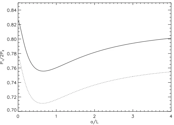
4.16 The ratio P1/2P2 for a sound wave in a non-isothermal loop of length 2L. The sound

speed squared varies linearly with distance, falling from a valuecapexat the loop apex to

cbase(=capex/λ)at its base. Whenλis close to unity the isothermal case is recovered

(cf. Fig. 4.14). . . 128 4.17 The ratioP1/2P2for a sound wave in a non-isothermal loop of length2L. Here the solid

line denotesL/Λc = 1.0and the dashed line isL/Λc = 2.0. Hereλ = capex/cbase is

varied. Notice that whenλ= 1thenP1/2P2 '0.95forL/Λc= 1.0andP1/2P2'0.85

forL/Λc = 2.0from Fig. 4.14. . . 128

4.18 Dispersion diagram for a coronal loop with apex 10 times hotter than its base (λ = 10).

Here,L/Λ0=αL. . . 131

(14)

density, and the dashed line indicates the maximum possible period for a homogeneous loop with density equal to the base density. . . 131 4.20 The period ratioP1/2P2as loop length varies for variouscapex/cbase =λ. Here the solid

line isλ= 1.5, the dashed line isλ= 3.0and the dotted line representsλ= 10.0. . . 132

4.21 The period ratioP1/2P2as the ratioλ=capex/cbasevaries. Fig. 4.20 shows that this ratio

is independent of loop length (here,αL= 1.0; however, this choice is arbitrary). . . 132

4.22 P1/2P2as a function of the scale heightL/Λc, for various chromospheric layers of

dimen-sionlessW/L(= 0.1,0.7,0.9). This diagram has been provided courtesy of A. J. D´ıaz and

is published in McEwan et al. (2006). . . 134

5.1 (a) A typical example of a large coronal loop footpoint supporting an oscillatory signal in TRACE 171 ˚A, from April 30th 2003, 1641UT. The footpoint is highlighted by the solid white lines. (b) Plot of the running difference taken over the time series at each position along the loop. The solid white lines indicate the gradient of the diagonal bands. . . 141 5.2 (a) The intensity oscillation in data numbers observed in a cut taken at positionp= 4along

the loop; this position shows the clearest evidence of an oscillation. The left hand diagram is the data including the background intensity trend, with the right hand side being the data with an average background level removed and the linear trend (dashed line) corrected for. (b) The wavelet diagram at position4along the loop. The dashed line indicates the cone

of influence and the solid lines indicate the contours of 99% confidence. The colour bar on the wavelet diagram shows that darker regions indicate the areas with higher normalised wavelet power. . . 142 5.3 Each mother wavelet,ψ, is plotted against a dimensionless period: (a) The Morlet wavelet

(Eq. (5.8)) withk= 6. (b) Paul wavelet (Eq. (5.9)) withk= 6. (c) DOG (or Mexican hat)

wavelet (see Eq. (5.10)) withk= 2. . . 145

5.4 (a) Function analysed using3different mother wavelets,f(t) = sin(2π10t)+sin(2π25t)+ sin(2π50t). (b) Wavelet power spectrum of the functionf(t)using a Morlet mother wavelet

withk = 6. (c) The power spectrum given whenf(t)is wavelet analysed using the Paul

mother wavelet withk= 6. (d) The wavelet diagram given whenf(t)is wavelet analysed

using the DOG mother wavelet withk = 6. The colour bars on the wavelet diagrams

indicate that darker regions have higher normalised wavelet power. . . 148 5.5 The function analysed using the same Morlet mother wavelet but with different wavelet

parameters,k, given by Eq. (5.14). . . 149

5.6 (a) Wavelet diagram forf(t)defined in Eq. (5.14) using the Morlet mother wavelet where

k = 3. (b) Wavelet diagram forf(t)using the Morlet mother wavelet wherek = 6. (c)

Wavelet diagram for f(t)using the Morlet mother wavelet where k = 9. (d) Wavelet

diagram forf(t)using the Morlet mother wavelet wherek = 12. The colour bars on the

wavelet diagrams indicate that darker regions represent higher normalised wavelet power. . 150 5.7 (a) Fast Fourier Transform (FFT) of Eq. (5.13), (b) FFT of Eq. (5.14). . . 151

(15)

5.8 Plot of the analytical Fourier transforms of Eq. (5.13), in blue, and Eq. (5.14) in red. Notice the Fourier power peaks at the frequenciesω0= 10,25and50present in the signal. . . 153

5.9 (a) The two sections of the wide fan-like coronal loop footpoint that are found to oscillate independently on June 13th 2001. The strand numbered 1 oscillates at 0057UT, whilst the strand numbered 2 oscillates at 0138UT. (b) The time-space diagram of the intensity running difference is takenacross(as opposed to along) the loop, labelled 3 in Fig. 5.9(a), at 0057UT on June 13th 2001. In this time-space diagram, position is defined to be the position along loop 3. At 0057UT the oscillation is mainly confined to around position10

across the loop structure, corresponding to strand 2 from Fig. 5.9(a). (c) The time-space diagram along loop3, taken on the same day at 0138UT. Now the intensity oscillation is

centred around position8, corresponding to strand1in Fig. 5.9(a). Note that the original

oscillation, at position10, is no longer present. . . 156

5.10 (b) The five coronal loop strands that oscillate on May 3rd 2003. The order in which these oscillate is given in Table 5.3. . . 159 5.11 (a) Active region AR0337 and the coronal loop footpoint supporting evidence of two

sim-ultaneous oscillations. (b) The running difference diagram showing the intensity variation, with the two sets of dark and light bands highlighted by the dashed lines. . . 162 5.12 (a) The intensity oscillation from the coronal loop footpoint studied on 26th April 2003,

showing evidence of two separate oscillations occurring simultaneously. Intensity is meas-ured along they-axis and time is measured in seconds along thex-axis. (b) The wavelet

diagram (taken at positionp = 3 along the loop) for the oscillation shows two bands of

period occurring throughout the dataset. The colour bar shows that darker regions on the wavelet diagram indicate higher normalised wavelet power. All subsequent wavelet dia-grams have the colour bar omitted. . . 163 5.13 (a) Histogram showing the distribution of the periods measured in this study. The dominant

period is clearly seen at around 300 s. There is a second peak at around200 s, as was

found by De Moortel et al. (2002b). (b) The histogram showing the distribution for all 63 examples observed. Here, the dominant period at around300s with a second peak at

around160s which is less pronounced. . . 168

A.1 (a) The running difference diagram showing intensity variation at 0057UT on June 13th 2001 on strand 1 of the wide coronal loop footpoint. (b) The running difference showing a similar variation in intensity at 0138UT on the same day, on strand 2. . . 178 A.2 (a) The wavelet diagram at 0057UT, using a Morlet mother wavelet withk= 6, showing a

periodic variation in intensity, present throughout the time series, of around350s. (b) The

wavelet diagram at 0138UT showing a period in intensity variation of around390s. The

darker regions on the wavelet diagrams indicate higher normalised wavelet power. . . 179 A.3 Figs. A.2(a), (b) and (c) show the coronal loop, time-space diagram and the clearest wavelet

diagram, at position 3, for the oscillation observed in Loop 1, from Table B.1. (d), (e) and (f) show loop 2, with wavelet diagram at position 2. (g), (h) and (i) show loop 3 (wavelet diagram at position 4) and (j), (k) and (l) show loop 4 at position 9. The darker regions on the wavelet diagrams indicate higher normalised wavelet power. . . 180

(16)

(f) show loop 6, taking the wavelet diagram at position 4. (g), (h) and (i) show loop 7 (wavelet diagram at position 0) and (j), (k) and (l) show loop 8 with the wavelet diagram at position 0. The darker regions on the wavelet diagrams indicate higher normalised wavelet power. . . 181 A.5 Figs. A.4(a), (b) and (c) show the coronal loop, time-space diagram and the clearest wavelet

diagram, at position 5, for the oscillation observed in Loop 9, from Table B.1. (d), (e) and (f) show loop 10, taking the wavelet diagram at position 4. (g), (h) and (i) show loop 11 (wavelet diagram at position 2) and (j), (k) and (l) show loop 12 with the wavelet diagram at position 1. The darker regions on the wavelet diagrams indicate higher normalised wavelet power. . . 182 A.6 Figs. A.5(a), (b) and (c) show the coronal loop, time-space diagram and the clearest wavelet

diagram, at position 1, for the oscillation observed in Loop 25, from Table B.1. The darker region on the wavelet diagram indicates higher normalised wavelet power. . . 186

(17)

Chapter 1 Introduction

“Many Bothans died to bring us this information.”, Mon Mothma

1.1 Overview of The Corona

1.1.1 Solar Interior and Lower Atmosphere

The Sun is a gaseous body of plasma, onion-like in structure, with near concentric layers defining regions of similar properties; see Fig. 1.1. In the solar core, which extends to about0.25R, whereRis the solar

radius, nuclear fusion of hydrogen provides the massive amount of energy required to power a star, around

99% of the Sun’s total energy. This nuclear fusion is possible as the pressure inside the core is so great,

under the massive pull of its own gravity. The energy is slowly leaking outwards, by radiative diffusion; however, the solar interior is so opaque that a photon leaking outwards would take107 _{million years to}

reach the surface (Priest, 1982; Lang, 2001). This region of radiative diffusion is called theradiative zone, which extends to about0.7R.

The temperature and density within the solar interior decrease rapidly as one moves away from the solar core, from a core temperature of around1.6×107K and density of₁_.₆_×₁₀5kg m−3to around₂_×₁₀6

K and200kg m−3_{at the top of the radiative zone. Above the radiative zone the temperature and density}

gradients becomes so large that the material can no longer be in static equilibrium, and convective motions begin to dominate the plasma. The region where this happens is called theconvection zone, which extends to the solar surface. The temperature drops to around6600K and the density drops to around4×10−4

kg m−3in this region. The temperature is now low enough that atomic recombination can occur, and the

photons, generated in the core by fusion, are absorbed by the plasma, leaving convection as the primary process for energy transportation. The base of the convection zone is believed to be a very important part of the Sun, called the tachocline(Spiegel and Weiss, 1980). The tachocline is thought to be the source of the dynamo process which generates the solar magnetic field. Above the convection zone lies the solar atmosphere, consisting of the photosphere, the chromosphere and the corona.

Thephotosphereis a thin, opaque layer of plasma, around0.5Mm in thickness, and it is this region that

emits most of the Sun’s light; see Fig. 1.2. The temperature at the top of the photosphere drops to around

4300 K and the density decreases to around8×10−5 kg m−3. The photosphere displays the granular

pattern of the solar surface, representing the top of the convective cells below, with diameters of around

1 Mm and lifetimes of around8minutes. Another photospheric structure is the sunspot, an area of such

(18)

[image:18.612.182.462.71.353.2]

Figure 1.1: Cartoon showing the solar interior (Lee, 2004), from the nuclear reactor that is the core, to the convective cells appearing on the solar surface, the photosphere.

high magnetic field that the temperature is decreased (Bray and Loughhead, 1964). These areas appear dark as they are cooler than the surrounding region. Sunspots have three parts, an inner dark umbra, a surrounding, brighter strand-like penumbra, and the superpenumbra, first discovered by Loughhead (1968). They typically appear in pairs, one spot is flux emerging and the other is flux submerging. The east-west orientation of the submerging-emerging sunspot pair is opposite in the northern and southern hemispheres, and switches every solar magnetic cycle. This phenomenon is known asHale’s polarity law.

Above the photosphere lies a narrow layer, around2.5Mm thick, called thechromosphere. The

temper-ature of the chromosphere begins to rise steadily, to around50000K. Above this is the region where the

most dramatic change in temperature takes place, thetransition region. Fig. 1.3 shows this dramatic change. Around1Mm in depth, the transition region lies between the chromosphere and the outer atmosphere of

the Sun, thecorona. This regions sees the temperature increasing dramatically to several million degrees Kelvin. The density drops to around10−10kg m−3. The corona, chromosphere and transition region are

(19)

1.1 Overview of The Corona 3

Figure 1.2: Image showing the granulation of the photosphere surrounding a sunspot (TRACE, 2003). Note the umbra and penumbra on the sunspot.

1.1.2 Solar Corona

During an eclipse the solar corona is observed as the faint halo surrounding the Sun. Fig. 1.4(a) shows an x-ray image of the corona and Fig. 1.4(b) shows the corona during an eclipse. The overall shape of the corona varies with the solar magnetic cycle, with few coronal holes present during sunspot minimum, as in Fig. 1.4(b). The corona itself extends out into deep space, far from the solar surface, to Earth and beyond. It interacts with the interplanetary gas and magnetic field. Parker (1958) described this constant streaming of solar plasma into interplanetary space as the Solar Wind. He discovered two solar wind solutions; the fast and slow solar wind. The wind is driven by the pressure difference between the solar plasma and the interplanetary gas (Kivelson and Russell, 1995). The coronal magnetic field can also be associated with the solar wind. The magnetic field can be defined by one of two categories: open field and closed field (Aschwanden, 2004). The open field is associated with the fast solar wind and the closed field is associated with the slow solar wind.

The corona is extremely hot and rare with temperatures well over1MK and densities of around10−12kg

m−3_{. The density can be enhanced in some coronal structures, for example; loops, streamers or arcades, or}

(20)

Figure 1.3: Plot of the temperature change in the solar atmosphere (MSU, 2002). Note the shallow transition region, in which the temperature increases at a great rate.

(a) (b)

Figure 1.4: (a) X-ray image taken by the Yohkoh satellite in 1992 (from Phillips (2000)). Large scale coronal holes, active regions, bright points and coronal loops can all be seen. (b) Image of the corona taken during a total eclipse (from NASA (2006)).

using the TRACE satellite, showing the loop structure of the magnetic field.

(21)

1.1 Overview of The Corona 5

Figure 1.5: (a) Typical example of a flaring coronal loop (TRACE, 1999), observed using TRACE. Flaring loops are highly dynamical and are often observed to rise out of a flare site, with plasma draining down to the footpoints as the plasma cools. (b) MDI magnetogram of the solar disk (SOHO, 2005), black areas are regions of positive magnetic flux and white areas are negative flux.

the corona in white light (see Fig. 1.4(b)).

Active regions, areas of enhanced magnetic activity and strength, are known to be the source of many of the coronal structures, such as the loops observed in Fig. 1.5(a). They appear as areas of complicated mag-netic fields in, for example, MDI magnetograms, an instrument onboard the SOHO satellite (see Fig. 1.5(b) for a typical full disk magnetogram). Active regions generally exist in two belts, within±30degrees of the

solar equator. In general they are bipolar (hence the black and white on the magnetogram). Some may exist for lifetimes of several tens of days, especially if they are associated with a sunspot. However, smaller act-ive regions may exist for only a few days. Actact-ive regions are not always directly associated with sunspots. Indeed, an active region can exist as a more diffuse region well after the sunspot has disappeared.

The temperature above active regions is generally enhanced compared to the surrounding plasma. In-deed, the corona above the active region can contain many different coronal loops, each at a different tem-perature. Observations in different wavelengths yield images of these various coronal loops, with typical temperatures between1and6MK. These loops are generally small in length and have lifetimes of typically

a few hours. They link areas within an active region. Large coronal loops may transcend active regions, and can be many100Mm in length, connecting regions of opposite polarity. Coronal loops are anchored

by the magnetic field at the tachocline, and motions from below could be a source of one of the phenomena associated with coronal loops, namely loop oscillations. The dimensions of coronal loops are an area of great study. Length is relatively easy to determine: a loop lies between one footpoint and the other, typically

50to several100Mm. The width of a loop is somewhat debated (for example Schmelz (2002); Schmelz

et al. (2003); Aschwanden and Nightingale (2005) and Aschwanden (2005) give recent discussions). Many observations yield widths of around8to10Mm; see Wang (2004) for example. However other findings

(22)

of order2to3Mm; see, for example, McEwan and De Moortel (2006). This topic is returned to in Chapter

5.

Other coronal structures are also frequently observed. For example, many coronal loops, all placed one after the other, in near parallel alignment, are known as a coronal arcade. They form a tunnel of hot loops, formed by plasma where the dominant magnetic field is reconnecting (Sweet, 1958; Parker, 1963; Priest and Forbes, 1986), releasing great energy, and heating the coronal arcade. This reconnecting field causes an outward moving eruption, or flare, of hot plasma, where electrons are accelerated to great energies. The hot corona represents a great problem in solar physics. It seems counter-intuitive that the corona, so far from the Sun’s nuclear powered core, should be so hot. In fact, the corona and its structures are continually heated, for example, if the heating mechanism was removed then a coronal loop would cool in a matter of only a few minutes. Theories other than magnetic reconnection have been proposed to explain coronal heating. For example, Heyvaerts and Priest (1983) proposed the corona may be heated by the phase mixing of Alfvén waves in regions of non-uniform Alfvén velocity and Porter et al. (1994a,b) studied the role of magnetoacoustic wave motions heating both the quiet corona and active regions. There exists extensive literature regarding the coronal heating problem, however, it is not a topic for this Thesis. For further information the reader is referred to recent reviews (and references therein) discussing many aspects of the coronal heating problem, for example, Erdélyi et al. (2003) and Klimchuk (2006).

One can also observe structures, called prominences, that are similar to clouds in the Earth’s atmosphere. These are cool, dense clouds of plasma, several hundred times cooler than the surrounding atmosphere (Tandberg-Hanssen, 1974). They are buoyant due to the magnetic field providing a tension force that is balanced against gravity. Prominences are long lived structures, that lie above the polarity inversion line – the line that divides regions of opposite magnetic polarities in the photosphere. They lie above coronal arcades, which connect the two regions of polarity. As with flares, prominences can also erupt spectacularly, with dramatic consequences on the surrounding plasma (Hirayama, 1974).

All coronal structures are governed by the magnetic field and its interaction with the plasma. One method of study of this interaction ismagnetohydrodynamics, or MHD for short. This branch of mathematics

and physics models the interactions and provides the necessary means to further the understanding of the processes involved. Key problems of MHD include the coronal heating problem, evolution of the magnetic field, and modelling coronal structures accurately. Throughout this Thesis the third of these problems is addressed, and particular motions within the plasma are utilised: oscillations and wave motions.

1.2 The MHD Equations

(23)

1.2 The MHD Equations 7

1.2.1 Maxwell’s Equations

Maxwell’s equations describe the change of the electric fieldEand the magnetic fieldBdue to the presence

of electric currents of densityjand electric charges of densityρc. The equations are

∇ ×B=µj+ 1

c2

∂E

∂t, (1.1)

∇ ×E=−∂_∂tB, (1.2)

∇.B= 0, (1.3)

∇.E= 1

ρc, (1.4)

where is the permittivity of free space and µis the permeability of free space. Eq. (1.1) is known as

Amp´ere’s Law, Eq. (1.2) is known as Faraday’s Law of Induction, Eq. (1.3) is the solenoidal condition, stating that there are no magnetic monopoles, and Eq. (1.4) is Gauss’s Law implying that charge is con-served;cis the speed of light in a vacuum.

Studying Eqs. (1.1) to (1.4) dimensionally, and considering l to be a typical lengthscale for plasma

variations, over a typical timescaleτ, then a typical plasma velocity will bev=l/τ. Next, using Eq. (1.2),

∇ ×E_∼ E

l , (1.5)

and also

∂B

∂t ∼ B

τ. (1.6)

Substituting these two estimates into Faraday’s Law of Induction (1.2) gives

E= l

τB=vB. (1.7)

Using these estimates in Amp´ere’s Law (1.1), then one obtains the relation

1

c2

∂E

∂t ∼

1

c2

E τ =

1

c2

v τB=

vl c2_{τ l}B=

v2

c2

B

l . (1.8)

Eq. (1.8) states that if plasma motions wherev care considered then the displacement current term ∂E/∂tcan be neglected from Amp´ere’s Law, i.e. consider non-relativistic motions, usually the case in the

corona.

The final electromagnetic equation to complete the set is Ohm’s Law,

j=σ(E+v_×B), (1.9)

whereσis the electrical conductivity. Ohm’s Law introduces the plasma velocity,v, and provides the bridge

(24)

Law (1.1) to eliminateEandjbetween Eqs. (1.1) and (1.4), gives

∂B

∂t =∇ ×(v×B) +η∇

2_B_, _(1.10)

where η = 1/(µσ)is the magnetic diffusivity (here assumed to be a constant). Eq. (1.10) is the MHD

induction equation. Comparing the first term of the right-hand side of Eq. (1.10) to the second gives the magnetic Reynolds number Rm = (vl)/η. Typically, in the corona,Rm 1as v andl are so large,

so one can consider the plasma to be perfectly conducting, or ideal. This condition describes the frozen flux theorem of Alfv´en (Alfv´en, 1943a): the magnetic field lines are frozen into the plasma, and as such they move with the plasma as it moves. In regions whereRm 1then the diffusive term of Eq. (1.10)

dominates, however, this limit mainly applies in regions with small typical lengthscales. In MHD the plasma velocity and the magnetic field are generally regarded as the primary variables, and the current and electric field are secondary.

1.2.2 Fluid Equations

The behaviour of the magnetic field described in the induction equation (1.10) is coupled to the behaviour of the plasma by Ohm’s Law (1.9). The motion of the continuous plasma is governed by the equations of continuity, motion and energy: the Navier-Stokes fluid equations. These equations can be deduced by taking moments of the Boltzmann equations for charged particles; however, as before, a continuous fluid is considered. Consider a typical lengthscalel and a timescaleτ over which the plasma varies, then the

plasma can be considered continuous if

lRL, (1.11)

that is, the lengthlover which the plasma varies macroscopically is very much greater than the ion

gyrora-dius,RL. Also, another requirement is the lengthscalel is very much greater than the mean free path of

an ion in the plasma, so that the plasma is contained by collisions of particles with neighbouring particles. If these conditions are satisfied then the plasma can be described using the hydrodynamic fluid equations. Firstly, the mass continuity equation for a fluid of densityρis,

∂ρ

∂t +∇.(ρv) = 0. (1.12)

The equation of motion is

ρDv

Dt =−∇p+F, (1.13)

where

D Dt ≡

∂

∂t+v· ∇. (1.14)

Here pis the plasma pressure and Frepresents the sum of all external forces. Typical external forces

(25)

1.2 The MHD Equations 9

(Braginskii, 1965), and gravityFg =−ρg.

The energy equation is given by (Priest, 1982)

ργ

γ−1

D Dt

_p

ργ

=−L, (1.15)

where pis the plasma pressure,γ is the ratio of specific heats (generally taken to be5/3in the corona)

andLis the energy loss function. In this Thesis an energy loss function which is adiabatic is considered,

i.e.L= 0and energy is conserved. This has a consequence on Eq. (1.15) which becomes

D Dt

p ργ

= 0. (1.16)

Finally, to complete the set of equations, an equation of state is required, the ideal gas law

p=R ˜

µρT, (1.17)

whereRis the gas constant andµ˜is the mean atomic weight. In hydrogenµ˜ = 0.5(the value used in this

Thesis), howeverµ˜= 0.6is also an acceptable value for the ionised solar corona.

1.2.3 Summary of the MHD Equations and Approximations

∂ρ

∂t +∇ ·(ρv) = 0, (1.18)

ρDv

Dt =−∇p+F, (1.19)

∂p

∂t +v· ∇p=−γp∇.v, (1.20)

p=R ˜

µρT, (1.21)

j= 1

µ∇ ×B, (1.22)

∇ ·B= 0, (1.23)

∂B

∂t =∇ ×(v×B) +η∇

2_B_. _(1.24)

Eqs. (1.18) to (1.24) are valid under the assumptions (Boyd and Sanderson, 1969; Priest, 1982):

1. charge neutrality is satisfied, i.e.ni−Nen, wherenis the total number density,niis the number

density of the ions andNeis the electron number density,

2. the lengthscales of macroscopic plasma variations are much greater than the gyrosynchotron radius of the charged particles,

(26)

corona, with a typical plasma number densityn = 1012 m−1 and temperature_T _{= 10}6 K, then

λc= 104m (Benz, 2002)),

4. the velocity of the macroscopic plasma motion is not relativistic,

5. the timescale of the relaxation of the particle distribution function to a Maxwellian takes place on a timescale of order the time between particle collisions.

Although MHD requires the plasma to be collisional, the corona is so rare that many structures are con-sidered collisionless. However, MHD actually provides reasonable descriptions of solar processes. In particular, for wave phenomena, the typical period of observed MHD waves is of the order of minutes but the collisional timescale of the plasma is of the order of a fraction of a second, so the plasma can be regarded as collisional in this case (see Schindler (2007) for a recent discussion of collisional and collisionless plas-mas). Other solar structures, or processes, satisfy this last assumption less rigorously, however, they are not discussed in detail in this Thesis.

1.3 MHD Waves

In a plasma, rarefactions and compressions result in variations of density, pressure and temperature, but also influence the magnetic field. In a perfectly conducting ideal plasma, the magnetic field and the plasma are frozen together (Alfv´en, 1943a), so any propagation of waves will result in variation of the magnetic field. Consider, briefly, the Lorentz force in the equation of motion (1.13),

j_×B= (∇ ×B)×B/µ= (B_{· ∇})B/µ− ∇ B2/(2µ)

, (1.25)

whereB=|B_|is the magnitude of the magnetic fieldB. In the presence of a magnetic field, together with

the plasma pressure gradient then there are three restoring forces: magnetic tension given by the first term on the right-hand side of Eq. (1.25); magnetic pressure given by the second term on the right-hand side of Eq. (1.25); and the plasma pressure. It is common to group together the plasma pressure and the magnetic pressure, producing the total pressure,pT.

In MHD three main types of wave motion are studied, all driven by different combinations of the restor-ing forces. The magnetic tension drives the Alfvén wave, first reported by Alfvén (1943b) and the plasma pressure and magnetic pressure drive compressional magnetoacoustic waves (Cowling, 1976). When these restoring forces combine then the three modes of oscillation become apparent: Alfvén waves and two mag-netoacoustic waves. The magmag-netoacoustic waves become acoustic waves in the absence of magnetic field. The presence of gravity further complicates these descriptions.

(27)

1.3 MHD Waves 11

for example, Cowling (1976), Priest (1982) and Roberts (1991). Their detection in the Sun’s atmosphere has recently been discussed in Erd´elyi et al. (2003), Aschwanden (2004), Wang (2004) and Nakariakov and Verwichte (2005).

1.3.1 Wave Speeds and Plasma-β

There are several intrinsic speeds associated with the MHD wave modes. Each speed is particular to a specific mode of oscillation and as such they define the modes themselves. The local sound speed csis

defined through

c2s=

γp0

ρ0

(1.26)

wherep0andρ0are the equilibrium pressure and densities of the plasma. Typically, in the solar corona the

sound speed is100−200km s−1, and it is at this speed that acoustic waves, driven by pressure perturbations,

propagate.

The local Alfv´en speedcAis defined through

c2A=

B2 0

µρ0 (1.27)

where B0 is the equilibrium magnetic field strength andµ is the magnetic permeability of free space.

Magnetic tension drives the Alfv´en waves along the magnetic field lines at this speed, typically1000−2000

km s−1in the corona.

The tube speedcT(see Roberts and Webb (1978)) is defined through

c2T=

c2 sc2A

c2 s+c2A

; (1.28)

cT is less than both the sound speed and the Alfv´en speed. The MHD slow mode, driven by magnetic

tension and pressure perturbations, propagates roughly along magnetic field lines at this speed.

The fast speedcfis defined through the sum of the squares of the Alfv´en and sound speeds,

c2f =c2s+c2A; (1.29)

cf is associated with the propagation speed of the fast MHD mode, driven by both magnetic tension and

pressure forces.cfis the highest wave speed from all the MHD modes.

Another important speed is the kink speedckgiven by (Ryutov and Ryutova, 1976; Spruit, 1981; Edwin

and Roberts, 1983; Roberts, 2000)

ck=

ρ0c2A+ρec2Ae

ρ0+ρe

1/2

(28)

whereρeis the environment density andcAeis the environment Alfv´en speed.

These speeds can be compared in magnitude to give simple reductions in the set of MHD equations. One such comparison is the plasma-β, the ratio of plasma pressure to magnetic pressure, given by

β= p0

B2 0/2µ

= 2c

2 s

γc2 A

. (1.31)

In much of the coronacs cA, as the plasma pressure is so small, this is a low-β plasma. Effectively

the plasma pressure terms can be neglected as the magnetic pressure is the dominant force here. A greater simplification is the cold plasma approximation, whereβ = 0. In effect the sound speed has been set to

zero, and as a consequence there are no plasma pressure perturbations and the acoustic and slow modes vanish. In the solar interiorβ 1and so the wave properties are switched. The effect of the magnetic

pressure is very small compared to the plasma pressure. In the outer corona the magnetic field strength is reduced, causing a reduction in magnetic pressure; thus the plasma-β can rise again, to values ofβ > 1,

discussed in Gary (2001). Therefore, most of the corona is a low-βplasma, sandwiched between regions

of high-β. In this Thesis low-βplasmas are considered in general.

1.3.2 Linearised MHD Equations

Consider the equation of motion, containing the Lorentz force but neglecting gravity, then the governing non-linear momentum equation is

ρDv

Dt =−∇p+ (B· ∇)B/µ− ∇ B

2_/₍₂_µ₎

. (1.32)

This equation, together with the mass continuity equation (1.18), the induction equation (1.24), withη= 0,

and the adiabatic energy equation (1.20) form the basis for this analysis.

Assume that there exists an equilibrium solution, where∂/∂t= 0, with no flows (i. e. v0= 0) so that

the density and magnetic field only vary spatially. In full, this equilibrium is given by

B0=B0ˆz, v0= 0, p0=constant, ρ0=constant, (1.33)

whereB0is also a constant. All equilibrium quantities are denoted by a subscript0.

Consider small perturbations about the equilibrium (1.33), with the perturbed quantities denoted by a subscript1,

B=B0+B1(z, t), v= 0 +v1(z, t), p=p0+p1(z, t), ρ=ρ0+ρ1(z, t). (1.34)

Linearising the equations of MHD gives insight into the behaviour of the system under small amplitude perturbations. This is done by substituting the total perturbed quantities given in Eq. (1.34) into the ideal MHD equations (1.32), (1.18), (1.24) withη = 0and (1.20). Subtracting the equilibrium solution (1.33)

(29)

ideal MHD equations in a uniform medium:

∂ρ1

∂t +ρ0∇ ·v1= 0, (1.35)

ρ0∂ v1

∂t =−∇p1+

1

µ(∇ ×B1)×B0, (1.36)

∂B1

∂t =∇ ×(v1×B0), (1.37)

∇ ·B1= 0, (1.38)

∂p1

∂t =−c

2

sρ0(∇ ·v1). (1.39)

Consider a uniform magnetic field,B0= (0,0, B0), with an Alfv´en speed

cA= √B0

µρ0. (1.40)

Differentiating Eq. (1.36) with respect totand eliminating∂B1/∂tusing Eq. (1.37) gives

∂2_v 1

∂t2 =−

1

ρ0∇

∂p1

∂t +

1

µ(∇ ×(∇ ×(v1×B0)))×B0. (1.41)

Substituting for∂p1/∂t, using the linearised energy equation (1.39), results in a single equation for the

velocity perturbation,v1:

∂2_v 1

∂t2 =c 2

s∇(∇ ·v1) +c2A

∇2vx+

∂ωz

∂y ,∇

2_v y−

∂ωz

∂x ,0

, (1.42)

wherev1= (vx, vy, vz)andωzis thez-component of the vorticity(∇ ×v1)given by

ωz= ∂vy

∂x − ∂vx

∂y . (1.43)

Thez-component of the curl of Eq. (1.42) reduces to the one dimensional wave equation

∂2_ω z

∂t2 =c 2 A

∂2_ω z

∂z2 . (1.44)

Consider a Fourier component in time, taking a plane wave of the form

ωz(x, y, z, t) =ωz0exp (i(ωt+kxx+kyy+kzz)) (1.45)

then the dispersion relation for the Alfv´en wave is obtained:

ω2=kz2c2A, (1.46)

that is,

(30)

where ω is the frequency and θ is the angle between the propagation vectork = (kx, ky, kz) and the

direction of the applied magnetic field (θ= 0indicates propagation along the field lines). The wave vector

kis of magnitudek= k2

x+ky2+kz2

1/2. The motions in the Alfv´en wave are perpendicular (transverse)

to the magnetic fieldBand involve no compression of the plasma.

Now introduce some notation for clarity (Lighthill, 1960, 1978),

∆ =∇ ·v1, (1.48)

Γ = ∂vz

∂z . (1.49)

Eq. (1.42) reduces by taking itsz-component together with the divergence of Eq. (1.48). This gives the

linear equations for the MHD modes of oscillation in an unbounded, uniform plasma (Lighthill, 1960; Roberts, 1981a), namely

∂2_v z

∂t2 =c 2 s

∂∆

∂z ⇒ ∂2_Γ

∂t2 =c 2 s

∂∆2

∂z2, (1.50)

∂2_∆

∂t2 = c 2 s+c2A

∇2∆−c2A∇2Γ. (1.51)

Eqs. (1.50) and (1.51), coupled with Eq. (1.44), allows v1 = (vx, vy, vz)to be fully defined in space

(Lighthill, 1960).

Eqs. (1.50) and (1.51) can be combined to give the single partial differential equation

∂4_∆

∂t4 − c 2 s+c2A

∂2

∂t2∇ 2_{∆ +}_c2

sc2A

∂2

∂z2∇

2_{∆ = 0}_, _(1.52)

with the same equation satisfied byΓ (Lighthill, 1960). In the absence of a magnetic field,c2

A = 0, so

integrating Eq. (1.52) twice with respect totand once with respect tozgives

∂2_v z

∂z2 −c 2 s

∂2_v z

∂z2 = 0. (1.53)

Eq. (1.53) highlights that in the absence of a magnetic field then Eq. (1.52) describes the acoustic wave.

Roberts (1981a) showed that by considering a Fourier component in time, taking a plane wave of the form

∆(x, y, z, t) = ∆0exp (i(ωt+kx+kyy+kzz)). (1.54)

then Eq. (1.52) could be written in the form

k2

x+ky2+m20= 0, (1.55)

where

m20=

k2 zc2s−ω2

k2

zc2A−ω2

(c2

s+c2A) (k2zc2T−ω2)

(31)

andcTis the tube speed, defined earlier in Eq. (1.28).

From Eq. (1.52) the dispersion relation for magnetoacoustic waves can be derived:

ω4−ω2k2 c2s+c2A

+kz2k2c2sc2A= 0. (1.57)

This relation has two solutions (it is a quadratic inω2_{), namely}

ω2=k

2

c2s+c2A

±h c2s+c2A

2

−4c2sc2Acos2θ

i1/2

. (1.58)

The positive sign gives the fast magnetoacoustic wave; the negative sign is the slow magnetoacoustic wave. In the absence of a magnetic field, cA = 0and the slow wave disappears (ω2 = 0), with the fast wave

becoming a pure sound wave (ω2 ₌ _k2_c2

s). Whencs = 0, the slow wave disappears, and the fast wave

speed becomes identical to the Alfv´en wave speed (ω2 ₌_k2_c2

A). From either Eq. (1.47) or Eq. (1.58) the

phase speedcph=ω/kof a mode can be obtained.

(a) (b)

Figure 1.6: Polar diagram of the phase speedcph = ω/kof the magnetoacoustic waves and the Alfv´en

wave. The phase speedcphis a function of the angleθ between the wave vectorkand the unperturbed

magnetic field,B0(aligned parallel to the horizontal axis). (a)cA> cs, (b)cs> cA.

Fig. 1.6(a) shows the phase speed of the three modes, wherecT ≤ cs < cA ≤ cf. It indicates that

the fast mode is not restricted to travelling along the magnetic field, but can propagate both parallel and perpendicular to the magnetic field or indeed at any angle to it; the fast wave is roughly isotropic. The slow and Alfv´en waves are field guided modes. They have their maximum speed when propagating exactly parallel to the field. In a low-βplasma, like the corona, the slow wave behaves like a field guided acoustic

wave.

(32)

1.4 Coronal Oscillations

It is now widely accepted, and indeed commonly observed, that MHD waves occur in the solar corona. With the advent of the SOHO and TRACE missions, these observations have become increasingly common, and increasingly useful in testing theoretical and numerical models. Indeed it was TRACE that brought about the first estimate of the magnetic field in a coronal loop (Nakariakov and Ofman, 2001), using a technique called coronal seismology, first proposed using Moreton waves by Uchida (1968), extended by Roberts et al. (1984) on theoretical grounds and illustrated using data from the radio band of observations. Prior to TRACE and SOHO there were no imaging satellites with a high enough temporal and spatial resolution to successfully identify oscillations in the corona. Observations were restricted mostly to the radio band; see Aschwanden (1987, 2004) for extensive reviews of radio observations of coronal oscillations. Several techniques have been used to look for coronal oscillations; for example, Wikstol et al. (1997) used the correlation between perturbed density, plasma pressure and plasma temperature together with the Doppler shift to look for signatures of wave propagation instead of the wave itself. By studying the Doppler shift it was possible to identify whether the wave was upward or downward propagating. Wave activity can also be observed by using UV line spectra, for example the method reported in McClements et al. (1991). Furthermore, the variation of the spectral line broadening from disk centre to the limb can be used to detect the dominant oscillations in coronal loops. Erdélyi et al. (1998) found that if Alfvén waves are dominant in a coronal loop then the line broadening from the centre to the limb increases, however, if magnetoacoustic waves dominate then the line broadening decreases. In this overview of observations of coronal oscillations the emphasis is on the post-TRACE/SOHO period, since which there has been an enormous increase in the number of oscillation observations. The literature surrounding the observations of coronal oscillations could fill many hundreds of pages; for further information, the reader is referred to various reviews, for example, see Erdélyi et al. (2003), Roberts (2004), Wang (2004), Aschwanden (2004), Nakariakov and Verwichte (2005) and De Moortel (2006).

1.4.1 Observations of Fast MHD Modes

Propagating fast MHD waves have proved difficult to observe, even with high temporal cadence telescopes such as TRACE. Typically the wavelength of a propagating wave will be much shorter than the structure guiding them; this implies very short periods. The time resolution of TRACE is normally around30s, but

it can be as little as4s (Handy et al., 1999). For a normal TRACE observing programme, the temporal

cadence will be around20to30s, allowing for observations of intensity oscillations with a period of around

2 to 3 minutes (Nakariakov and Verwichte, 2005), far too long for the expected periods of propagating fast waves. So the current generation of EUV imaging telescopes are inadequate in this respect. Better temporal resolution can be obtained by using ground-based coronographs, such as the SECIS (Solar EClipse Imaging System) instrument.

The SECIS instrument was used by Williams et al. (2001, 2002), during a solar eclipse, to observe very rapid compressible wave trains, propagating along coronal loops on the solar limb. The waves travelled with a speed of around2100km s−1_{, a speed indicative of the fast MHD mode. The periodicity associated with}