A hyper heuristic approach to automated generation of mutation operators for evolutionary programming

A Hyper-heuristic Approach to Automated Generation of Mutation

Operators for Evolutionary Programming

Libin Honga_{, John H. Drake}b_{, John R. Woodward}c_{, Ender ¨Ozcan}a

a_{School of Computer Science, University of Nottingham}

b_{Operational Research Group, School of Electronic Engineering and Computer Science,}

Queen Mary University of London, E1 4NS, UK

c_{Computing Science and Mathematics, University of Stirling}

Abstract

Evolutionary programming can solve black-box function optimisation problems by evolving a

pop-ulation of numerical vectors. The variation component in the evolutionary process is supplied by

a mutation operator, which is typically a Gaussian, Cauchy, or L´evy probability distribution. In

this paper, we use genetic programming to automatically generate mutation operators for an

evo-lutionary programming system, testing the proposed approach over a set of function classes, which

represent a source of functions. The empirical results over a set of benchmark function classes

illustrate that genetic programming can evolve mutation operators which generalise well from the

training set to the test set on each function class. The proposed method is able to outperform

exist-ing human designed mutation operators with statistical significance in most cases, with competitive

results observed for the rest.

Keywords: Evolutionary Programming; Genetic Programming; Automatic Design;

Hyper-heuristics; Continuous Optimization

1. Introduction

Black-box function optimisation is the task of finding the optima of an objective function for

which we do not have access to an analytical form. A generate-and-test approach can be used

to sample the domain of the function in order to identify potential optima. Different black-box

optimisation techniques have been proposed; the majority of which are the result of much manual

effort. In addition, each optimisation algorithm is designed in isolation from a problem environment.

A proposed algorithm is usually tested on a number of benchmark functions to demonstrate its

a parameterised function in which the parameters have a certain range of values. Thus a function

class represents an infinite source of functions, from which it is possible to draw sets of sample

functions from the same distribution.

This paper is concerned with evolutionary programming (EP) [1], which evolves a population

of real-valued input vectors for a function, a technique widely applied to real-world problems [2,

3, 4]. As EP has an evolutionary basis, each vector undergoes selection, evaluation, and mutation,

with the expectation that fitter and fitter vectors are obtained. Here we focus on the mutation

component of EP, which in the past has been designed manually. Real-valued optimisation is an

active research topic and several population-based metaheuristics have been applied to function

optimisation, including differential evolution and its variants [5, 6] , particle swarm optimisation

[7], covariance matrix adaptation evolution strategy (CMA-ES) [8] and hybrid methods [9]. We

acknowledge the existence of these algorithms. However, as this study is concerned specifically

with the modification of EP, a full review of all of these algorithms is beyond the scope of this

paper.

A hyper-heuristic is a search method or learning mechanism for selecting or generating heuristics

to solve computational search problems [10]. In addition to the broad distinction between selection

and generation hyper-heuristics, it is also possible to classify hyper-heuristics according to the

source of feedback during learning. Online hyper-heuristics learn while solving a given instance of

a problem, whilst hyper-heuristics which learn in anoffline manner gather knowledge in the form

of rules or programs, from a set of training instances, that would hopefully generalise to the process

of solving unseen instances. genetic programming (GP) [11] is a population-based evolutionary

computation method for evolving program trees, that has frequently been used as a generation

hyper-heuristic in the literature [12].

In this paper, we use GP as an offline generation hyper-heuristic to automatically create

mu-tation operators for EP operating on function classes. A mumu-tation operator in EP is a probability

distribution, represented as a random number generator. We present an algorithmic framework

which can not only express a number of currently existing EP mutation operators, but also

gen-erate novel variants of EP mutation operators. Using a train-and-test approach, GP is used to

evolve mutation operators for EP, using a training set drawn from a class of functions which is

then validated on a larger set of unseen instances taken from the same class. We use the term

by GP. We demonstrate that the ADMs for EP are capable of comparable, and often superior,

performance to existing human designed operators. An additional set of experiments that takes

ADMs that are trained on one function class, but then tested on a different function class is also

conducted to further examine the performance of the evolved ADMs.

The outline of the remainder of this paper is as follows. In Section 2, we give the background

to the proposed approach of automatically designing algorithms using GP-based hyper-heuristics.

In Section 3 we consider the task of function optimisation and introduce the notion of a function

class. Section 4 presents our experimental results, which are analysed in Section 5. In Section 6

we discuss the research presented and in Section 7 we summarise the article and outline potential

further research directions.

2. Automated Design Using Hyper-Heuristics

The key distinction between metaheuristics and hyper-heuristics is that the former operate

directly on the solution search space, while the latter operate indirectly on the solution search

space, working with a set of low-level heuristics or heuristic components. Hyper-heuristics come in

two main types: heuristics to choose heuristics and heuristics to generate heuristics [10]. In this

paper we are concerned with the second of these two categories, heuristics to generate heuristics [12].

The automated generation of heuristics has received much attention in the last few years.

Wood-ward et al. [13] automatically search the space of genetic algorithm (GA) selection operators, which

contain fitness proportional and rank selection, where bitstrings in the population are chosen in

proportion to their fitness value or indexed position in the sorted population respectively. In a later

paper by the same authors, novel mutation operators were automatically constructed using random

search and multiple-restart hill-climbing to search the space of mutation operators [14]. The

sys-tem was capable of expressing two well-known mutation operators: one-point anduniform. While

random search and hill-climbing may not be considered to be particularly ‘sophisticated’, they

were sufficient to discover new selection and mutation operators which outperformed their human

designed counterparts. Diosan and Oltean [15] evolved crossover operators for genetic algorithms

outperforming existing crossover operators on some function optimisation problems.

As one of the main applications areas of metaheuristics is combinatorial optimisation problems,

it is not surprising that this type of problem has attracted the attention of automated design.

used GP to automatically design algorithms for job-shop scheduling, Keller et al. [17] tackled the

travelling salesman problem, while Bader El Den et al. [18, 19] evolved timetabling heuristics.

Drake et al. [20] used GP to evolve a scoring mechanism to determine the order in which knapsack

items should be considered by a constructive heuristic for the multidimensional knapsack problem.

Hong et al. [21] used GP to automate the design of probability distributions as mutation operators

for evolutionary programming. GP was used to generate new data mining algorithms which were

tested on well-known machine learning benchmark datasets by Freitas and Pappa [22]. Their paper

showed that GP could outperform random search in searching the space of rules for data mining.

The rules evolved by GP were observed to be at least as good as human designed rules in terms

of classification. GP has also been used to automatically design schedule policies for dynamic

multi-objective job shop scheduling [23], to evolve ensembles of dispatching rules for the job shop

scheduling problem [24], and to automate the design of production scheduling heuristics [25]. Both

online and offline bin packing have attracted attention within the heuristic generation research

community [26]. Heuristic functions have been evolved to determine in which bin to place a given

item [27]. In this case, the evolved heuristic functions have been shown to perform well on problem

instances drawn from the same problem class used in the training phase, while a degradation in

performance is witnessed when heuristics are applied to problem instances drawn from different

problem classes. Heuristics have been evolved on problem instances containing a small number of

items, then applied to much larger problem instances containing many more items [28]. In these

approaches, a heuristic function is evolved as a GP syntax tree. However, more recently, both

a look-up table (referred to as a “matrix”) [29, 30] and function interpolation [31] have also been

used to represent a heuristic function. Other metaheuristics have been automatically designed using

hyper-heuristics, such as particle swarm optimisation [32] and variable neighbourhood search [33].

This current paper builds on previous papers. Hong et al. [21] first demonstrated that GP could

automatically construct random number generators which are typically used in EP. In a second

paper, it was shown that ADMs could be trained on collections of functions classes, showing good

performance across a broader range of functions [34], however a tradeoff between general training

and specific performance was observed. This paper presents a study of the design of 23 ADMs, for

3. Optimisation and Function Classes

In this section we first discuss optimisation with EP, and then introduce function classes as

probability distributions over functions. Function classes are central to this paper, differentiating

our approach from the standard convention of benchmarking on arbitrary functions. Rather than

demonstrating the utility of an optimisation algorithm for specific arbitrary functions, we

demon-strate the utility of an ADM on a set of functions are drawn from a fixed probability distribution

(i.e. a function class).

3.1. Evolutionary Programming and Optimisation

We follow the formulation of optimisation as stated by Yao et al. [1, 35], which we repeat here.

Global minimisation can be formalised as a pair (X, f), whereX∈Rn is a bounded set inRn and

f :X →Ris ann-dimensional real-valued function. The objective is to find a pointxmin∈X such

thatf(xmin) is a global minimum inX. More specifically, it is required to find an xmin such that

∀x∈X :f(xmin)≤f(x).

Here,f does not need to be continuous or differentiable. While the aim of optimisation is to identify

global optima of the function, in practice we often settle for methods, such as EP, which identify

near-optima. EP is a widely used evolutionary algorithm for continuous optimisation introduced

by B¨ack and Schwefel [36] as follows:

1. Generate the initial population of µ individuals. Each individual is taken as a pair of

real-valued vectors, (xi, ηi), ∀i ∈ {1, . . . , µ}, where xi’s are objective variables and ηi’s are standard

deviations for Gaussian mutations.

2. Evaluate the fitness value for each (xi, ηi), ∀i ∈ {1, . . . , µ}, of the population based on the

objective function,f(xi).

3. Each parent (xi, ηi), ∀i ∈ {1, . . . , µ}, creates λ / µ offspring on average, so that a total

of λ offspring are generated. Offspring are generated by: for i ∈ {1, . . . , µ}, j ∈ {1, . . . , n} and

p∈ {1, . . . , λ},

η_i0(j) =ηi(j)exp(γ0N(0,1) +γNj(0,1)) (1)

x0p(j) =xi(j) +η0p(j)Dj (2)

where xi(j), x0_p(j), ηi(j) and η_p0(j) denote the j-th component of the vectors xi, x0_p, ηi and η_p0

and standard deviation 1. Nj(0,1) indicates that the random number is generated anew for each

value ofj. The factorsγ andγ0 are set to (p2√n)−1 _and(√_2n)−1 _[36].

4. Calculate the fitness of each offspring (x0_p, η0_p),∀p∈ {1, . . . , λ}, according to f(x0_p).

5. Conduct pairwise comparison over the union of parents (xi, ηi) and offspring (x0_p, η_p0), ∀i∈

{1, . . . , µ},∀p∈ {1, . . . , λ}. For each individual,qopponents are selected randomly from the parents

and offspring. For each comparison, if the individuals’ fitness is no smaller than the opponent’s it

receives a ‘win’.

6. Select theµindividuals out of the parents and offspring ((xi, ηi) and (x0p, ηp0),∀i∈ {1, . . . , µ},

∀p∈ {1, . . . , λ}) that have the most wins to be the parents of the next generation.

7. Stop if the halting criterion is satisfied; otherwise return to Step 3.

Different variants of EP can be obtained by using different probability distributionsDj in Step

3 above. If Gaussian distribution is used, then the algorithm is classical evolutionary programming

(CEP) [1], the Cauchy distribution is used in Fast EP (FEP) [1] whereas the L´evy distribution is

used in L´evy evolutionary programming (LEP) [37]. The L´evy distribution is parameterised with

a single parameterα, and corresponds to the Cauchy distribution when α=1.0 and the Gaussian

distribution when α=2.0. Where LEP is used in this paper, the L´evy Lα,γ(y) distribution is

implemented according to Mantegna [38] as given by Lee and Yao [37], withγfixed at 1 (note that

γhere is independent from step 3 above):

Lα,γ(y) = 1

π

Z ∞

0

e−γqαcos(qy)dq, y∈R. (3)

In this paper we will use genetic programming to evolve distributions to replaceDj as a mutation

operator in the EP system described above. In each case, we use the same parameters for EP as

previous publications [1, 35], using tournament selection with tournament size 10 on a population of

100 individuals. The initial value of the strategy parameterηis set to 3.0.The number of generations

is different for each function and is specified in Table 1 below.

3.2. Functions and Function Classes

In previous papers [35, 37, 39, 40], methods have been compared on functions from an arbitrary

set. Each method is executed multiple times on asinglefunction to provide a statistical comparison.

representing a probability distribution over a set functions. An example of a function class is

y=ax2 _{wherea is uniformly distributed in the range [1, 2]. In this case,y = 1.3x}2 _{is a function}

from this function class, whiley= 0.3x2_{is not from this function class. For each of the 23 standard}

functions often used in EP research [1, 35], we have constructed a corresponding function class.

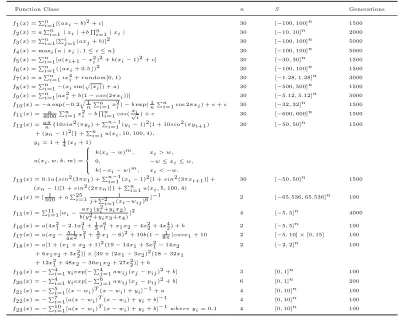
The 23 benchmark function classes are given in Table 1. These can be classified as follows: f1–f7

are unimodal functions,f8–f13 are multimodal functions with many local optima, andf14–f23are

multimodal function with few local optima [35].

Table 1: Function classes with number of dimensionsn, domainS, and number of generationsGen. The parametersa,b

andcare uniformly distributed in [1 ,2], [-1, 1] and [-1, 1], respectively. For the values ofwinf19tof23, please see [35]

Function Class n S Generations

f_{1 (}x) =Pn

i=1[(axi−b)2 +c] 30 [−100,100]n 1500

f2 (x) =aPn

i=1|xi|+b

Qn

i=1|xi| 30 [−10,10]n 2000

f_{3 (}x) =Pn

i=1[

Pi

j=1(axj+b)]2 30 [−100,100]n 5000

f4 (x) = maxi{a|_xi|,1≤i≤n} 30 [−100,100]n 5000

f5 (x) =Pn

i=1[a(xi+1−x2i)2 +b(xi−1)2 +c] 30 [−30,30]n 1500

f_{6 (}x) =Pn

i=1(baxi+ 0.5c)2 30 [−100,100]n 1500

f7 (x) =aPn

i=1ix4i+random[0,1) 30 [−1.28,1.28]n 3000

f_{8 (}x) =Pn

i=1−(xisin(

p

|xi|) +a) 30 [−500,500]n 1500 f9 (x) =Pn

i=1[ax2i+b(1−cos(2πxi))] 30 [−5.12,5.12]n 5000

f_{10 (}x) =−aexp(−0.2

q

1 n

Pn

i=1x2i)−bexp( 1n

Pn

i=1cos 2πxi) +e+c 30 [−32,32]n 1500

f11 (x) =₄₀₀₀a Pn i=1x2i−b

Qn

i=1cos(√xii) +c 30 [−600,600]

n ₁₅₀₀

f12 (x) =aπ_n{10sin2 (πyi) +Pn−1

i=1(yi−1)2 [1 + 10sin2 (πyi+1 ) + (yn−1)2 ]}+Pn

i=1u(xi,10,100,4), yi= 1 + 1₄(xi+ 1)

u(xi, w, k, m) =

        

k(xi−w)m , xi > w,

0, −w≤xi≤w,

k(−_xi−w)m , xi <−w.

30 [−50,50]n 1500

f_{13 (}x) = 0.1a{sin2 (3πx_{1 ) +}Pn−1

i=1(xi−1)2 [1 +sin2 (3πxi+1 )] + (xn−1)[1 +sin2 (2πxn)]}+Pn

i=1u(xi,5,100,4)

30 [−50,50]n 1500

f14 (x) = [₅₀₀1 +aP25

i=1j+P₂ 1

i=1(xi−wij)6

]−1 2 [−65.536,65.536]n 100

f15 (x) =P11 i=1[wi−

ax1 (y_i2+yix2 ) b(y_i2+yix3 +x4 )

]2 4 [−5,5]n 4000

f16 (x) =a(4x2₁−2.1x4_{1 +}1₃x6_{1 +}x1x2−4x2_{2 + 4}x4_{2 ) +}b 2 [−5,5]n 100

f17 (x) =a(x2−_4π5.12x21 +π5x1−6)2 + 10b(1− 1

8π)cosx1 + 10 2 [−5,10]×[0,15] 100

f18 (x) =a[1 + (x1 +x2 + 1)2 (19−14x1 + 3x2₁−14x2 + 6x1x2 + 3x2_{2 )]}×[30 + (2x1−3x2 )2 (18−32x1 + 12x2_{1 + 48}x2−36x1x2 + 27x2_{2 )] +}b

2 [−2,2]n 100

f19 (x) =−P4

i=1yiexp[−

P4

j=1awij(xj−pij)2 +b] 3 [0,1]n 100

f_{20 (}x) =−P4

i=1yiexp[−

P6

j=1awij(xj−pij)2 +b] 6 [0,1]n 200

f21 (x) =−P5

i=1[(x−wi)T(x−wi) +yi]−1 +a 4 [0,10]n 100

f22 (x) =−P7

i=1[a(x−wi)T(x−wi) +yi+b]−1 4 [0,10]n 100

f_{23 (}x) =−P10

i=1[a(x−wi)T(x−wi) +yi+b]−1where yi= 0.1 4 [0,10]n 100

4. Experimental Design

In this section we describe the experimental set-up of GP and EP. With hyper-heuristic

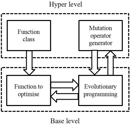
Figure 1: Overview of the hyper-heuristic framework used

hyper-heuristic, a metaheuristic operates on a space of (meta) heuristics, which operate directly

on the space of solutions. Here we use GP as a mutation operator generator at the hyper-level to

manipulate the mutation operators within a population of EP algorithms working at the base level.

The overall framework used is given in Figure 1.

Previous approaches manually build optimisation methods and test them on benchmark

func-tions [1, 35]. Here we employ a train-and-test approach, in which a first set of funcfunc-tions is used to

train a method before it is tested on a second independent set of functions drawn from the same

probability distribution to analyse performance.

4.1. The Training Phase

We call a program generated by GP an ‘automatically designed mutation operator’ (ADM),

which is in effect a random number generator. Each ADM is used as an EP mutation operator on

5 training functions drawn from a given function class. The fitness of an ADM is the average of

the best values obtained in each of the individual 5 EP runs on a given function class. We use the

each function class, 10 functions are taken for training, 5 of which are used to calculate the fitness,

and 5 of which are used to monitor overfitting.

4.2. The Testing Phase

When the training phase of EP is complete for a given function class, the output is an ADM

intended solely for the function class on which it was trained. We then draw 50 new functions

from the given function class and test the ADM, comparing against 6 existing EP variants (CEP,

FEP and EP with 4 settings for the α parameter of the L´evy distribution). Note that training

is expensive, as many ADMs are evaluated, so a small set of functions is used when training. In

contrast, testing involves only a single ADM so is less costly, and a larger number of testing samples

allows a better comparison through statistical tests.

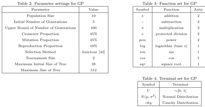
4.3. Parameter Settings for Genetic Programming

The GP implementation used in this paper is the genetic programming toolbox for Matlab

(GPLAB) [41]. The parameters for GP are given in Table 2. We use subtree crossover, in which

a node in each of the parent programs is chosen uniformly at random, and the respective subtrees

are swapped, creating two new offspring. One point mutation is also used, where a node is chosen

in the parent tree and substituted for a new tree created with the Grow initialisation method [11],

obeying the size and depth restrictions imposed by the GP parameters. The fitness of each GP

individual is calculated as the average best fitness values of the EP runs on each of the 5 training

functions, as described in Section 4.1 above. At each generation, the best individual from both

parents and offspring, along with the best offspring created during that generation are retained

in the population. The selection method used is ‘lexictour’, which uses lexicographic parsimony

pressure when two individuals are compared [42], if two individuals are of equal fitness, the tree

with a smaller number of nodes is chosen. As the evolutionary process is incredibly expensive

in computational terms (each GP individual has to perform 5 EP runs), the maximum number

of generations is initially set at a low value to reduce the amount of computational effort spent.

The maximum number of generations is set dynamically to try to ensure that a sufficient number

of evaluations are made to achieve convergence, whilst minimising the time spent on evaluating

poor quality runs. If the best individual in the population is found within the final three

evolutionary process to continue. The maximum number of generations is capped at 100, with the

evolutionary process terminated regardless of when the best individual in the population was found.

Table 2: Parameter settings for GP

Parameter Value

Population Size 10

Initial Number of Generations 5

Upper Bound of Number of Generations 100

Crossover Proportion 45%

Mutation Proportion 45%

Reproduction Proportion 10%

Selection Method lexictour [42]

Tournament Size 2

Maximum Initial Size of Tree 28

Maximum Size of Tree 512

Table 3: Function set for GP

Symbol Function Arity

+ addition 2

− subtraction 2

× multiplication 2

÷ protected division 2

pow power 2

log logarithm (base e) 1

sin sin 1

cos cos 1

sqr square root 1

Table 4: Terminal set for GP

Symbol Terminal

U ∼[0, 1]

N(µ, σ2_{) Normal Distribution}

chy Cauchy Distribution

The function and terminal sets for GP are given in Tables 3 and 4, respectively. U is the

uniform distribution on [0, 1]. N(µ, σ2_{) is the normal distribution with mean µand variance σ}2_.

Here we clarify that thisµis independent to that used in the EP descriptions in Section 3 In our

experiments,µlies within the range [-2, 2] andσ2_{is in [0, 10]. chyis the Cauchy distribution. ‘÷’ is}

protected divide: if the numerator is divided by a zero denominator, then the numerator is returned.

The square root function is also the protected variant, taking the square root of the absolute value

of a single argument to ensure that no negative input is used. As the L´evy distribution can be

constructed from the normal distribution and arithmetic operators [38], it is also within the search

space that GP is operating in. In the terminal set there are no input variables, here we are using GP

to construct mutation operators which are effectively random number generators so do not require

any input variable.

5. Analysis of the Performance of the Automatically Designed Mutation Operators

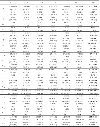
Table 5 reports the average best values obtained over 50 EP runs of each of the 23 function

classes using a number of different mutation operators. The corresponding standard deviations are

L´evy withα= 1.0), L´evy withα= 1.2,α= 1.4,α= 1.6 andα= 1.8, and Gaussian (CEP, L´evy

with α= 2.0), as well as the best ADM evolved by GP for that function class. The best values

(lowest, as we are minimising) are in boldface.

Table 5: ADMs compared to human designed mutation operators, means and (standard deviations), averaged over 50 runs.

The best fitness values are in bold.

Cauchy α= 1.2 α= 1.4 α= 1.6 α= 1.8 Gaussian ADM

f1

6.012303 6.011758 6.011538 6.011426 6.011369 6.011267 6.011234

(15.5123) (15.5123) (15.5123) (15.5123) (15.5123) (15.5123) (15.5123)

f2

0.140 0.102 0.084 0.073 0.065 0.043 0.017

(2.8E-02) (2.0E-02) (1.7E-02) (1.5E-02) (1.3E-02) (8.6E-03) (3.5E-03)

f3

0.028 0.018 0.014 0.015 0.018 0.018 0.008

(2.0E-02) (2.2E-02) (1.8E-02) (3.4E-02) (5.3E-02) (2.6E-02) (1.4E-02)

f4

1.88 5.30 9.10 10.58 13.78 17.31 0.13

(1.87) (3.49) (4.36) (4.43) (6.56) (6.92) (0.21)

f5

-19.94 -19.87 -20.42 -20.21 -19.61 -20.22 -20.63

(26.13) (26.51) (26.94) (25.71) (26.44) (26.35) (27.15)

f6

0.0336 0.0134 0.0076 0.0724 0.9058 322.7146 0.0074

(3.0E-02) (1.3E-02) (8.2E-03) (2.4E-01) (2.87) (820.2) (9.4E-03)

f7

0.0586 0.0530 0.0506 0.0524 0.0554 0.0609 0.0486

(9.3E-03) (8.6E-03) (7.9E-03) (6.9E-03) (9.9E-03) (1.1E-02) (6.3E-03)

f8

-11058.28 -10642.83 -10009.65 -9530.88 -8818.26 -8053.96 -12469.12

(397.2) (507.5) (483.6) (586.8) (645.2) (603.5) (109.0)

f9

-10.953 -10.955 -10.956 -10.956 -10.357 -8.269 -10.958

(15.82) (15.82) (15.82) (15.82) (16.21) (16.29) (15.82)

f10

-27.8428 -27.8496 -27.8529 -27.8549 -27.8562 -27.7300 -27.8634

(6.86) (6.87) (6.87) (6.87) (6.87) (6.93) (6.87)

f11

-0.4963 -0.4839 -0.4704 -0.4534 -0.4554 -0.4465 -0.5030

(6.4E-01) (6.4E-01) (6.5E-01) (6.7E-01) (6.4E-01) (6.3E-01) (6.4E-01)

f12

1.72E-05 2.13E-02 1.82E-01 1.77E-01 1.01 2.37 3.57E-06

(8.8E-06) (5.9E-02) (4.7E-01) (3.7E-01) (2.0) (2.9) (2.5E-06)

f13

2.20E-04 5.20E-04 2.87E-01 5.67E-01 2.23 7.04 6.46E-05

(5.5E-05) (2.7E-03) (1.5) (1.6) (6.9) (13.0) (2.3E-05)

f14

1.32 0.98 1.24 1.08 1.11 0.90 0.78

(1.1) (6.9E-01) (8.1E-01) (7.1E-01) (6.0E-01) (5.1E-01) (2.9E-01)

f15

5.68E-04 5.13E-04 5.90E-04 6.03E-04 6.34E-04 5.39E-04 4.66E-04

(3.6E-04) (3.2E-04) (3.8E-04) (3.5E-04) (3.9E-04) (3.3E-04) (3.1E-04)

f16

-1.522775 -1.522775 -1.522776 -1.522776 -1.522776 -1.522777 -1.522779

(0.6049959) (0.6049966) (0.6049960) (0.6049964) (0.6049962) (0.6049962) (0.6049964)

f17

5.8792588 5.8792572 5.8792571 5.8792674 5.8792569 5.8792566 5.8792563

(2.9140509) (2.9140486) (2.9140487) (2.9140637) (2.9140487) (2.9140488) (2.9140489)

f18

4.615353 4.615353 4.615322 4.615324 4.615301 4.615228 4.615192

(0.9234) (0.9235) (0.9234) (0.9234) (0.9234) (0.9234) (0.9234)

f19

-3.353969 -3.354014 -3.354021 -3.354022 -3.354025 -3.354040 -3.354058

(1.7371) (1.7370) (1.7370) (1.7370) (1.7370) (1.7370) (1.7371)

f20

-3.67 -3.73 -3.83 -3.56 -3.76 -3.74 -3.86

(2.15) (2.30) (2.24) (2.13) (2.25) (2.18) (2.25)

f21

-4.33 -5.99 -5.59 -5.84 -6.44 -6.96 -7.26

(2.0) (2.7) (2.7) (2.8) (2.5) (2.4) (2.2)

f22

-11910.70 -23968.23 -20517.80 -20734.62 -12662.55 -68694.69 -85515.41

(25106.9) (70957.4) (36414.1) (35143.6) (20568.8) (193492.5) (195260.3)

f23

-20808.83 -19096.31 -14155.95 -18304.26 -20858.36 -27047.33 -111864.57

For all 23 of the function classes, the GP designed ADM outperform the 6 human designed

mutation operators. In Table 5 the evolved ADMs show the best performance on both unimodal

and multimodal functions generated by all listed function classes in Table 1. We retain 2, 3 or 4

digits after the decimal point for most of the results. To distinguish the difference of testing results

onf1,f16 andf18, we retain 6 digits after the decimal point. We retain 7 digits after the decimal

point for testing results onf17.

To determine which of these performances differ with statistical significance, we perform a

Wilcoxon signed-rank test, the results of which are presented in Table 6. Shown are the results

of the Wilcoxon signed-rank test within a 95% confidence interval of an ADM compared with

other mutation operators. In this table, ‘≥’ indicates that the ADM performs better than another

mutation operator on average. In the cases where this difference is statistically significant, ‘>’

is used. In the majority of the cases, the ADMs outperform human designed mutation operators

including Gaussian, Cauchy and L´evy, and this performance difference is statistically significant.

Table 6: Wilcoxon Signed-Rank Test of ADMs versus Gaussian, Cauchy and L´evy (withα= 1.2, 1.4, 1.6, 1.8) onf1–f23.

Function Class Cauchy α= 1.2 α= 1.4 α= 1.6 α= 1.8 Gaussian

f1 > > > > > >

f₂ > > > > > >

f3 > > > ≥ ≥ >

f₄ > > > > > >

f5 ≥ ≥ ≥ ≥ ≥ ≥

f₆ > > ≥ > ≥ >

f7 > > > ≥ > >

f8 > > > > > >

f9 > > > > > >

f10 > > > > > >

f11 > > > > > >

f12 > > > > > >

f₁₃ > > > > > >

f14 ≥ > > > > >

f₁₅ > > > > > >

f16 > > > > > >

f17 > > > > > >

f18 > > > > > >

f19 > > > > > >

f20 > > > ≥ > >

f21 > > > > > ≥

f₂₂ > > > > > >

f23 > > > > > >

There are only 2 (f5, f14), 1 (f5), 2 (f5, f6), 4 (f3, f5, f7, f20), 3 (f3, f5, f6) and 1 (f5)

function classes for which evolved ADMs perform slightly better than Cauchy, Levyα=1.2, Levyα=1.4,

a number of reasons. It is possible that EP has been run for so many iterations that it does not

matter which mutation operator is used, and any difference in performance is negligible. It also

may be the case that GP would be able to find better mutation operators if it were allowed to run

for a longer period of time. One reason that GP can consistently find ADMs which perform at least

as well as human designed mutation operators is that they are easily expressed within the function

and terminal set used.

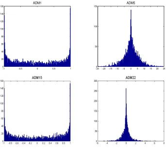
The best ADMs obtained with GP for each function class are listed in Table 7. Figure 2 provides

histograms for a subset of ADMs, showing 3000 samples taken from the ADM to give an indication

of the underlying probability distribution they represent.

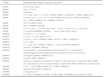
Table 7:Evolved ADMs for all 23 function classes. These have been algebraically simplified where possible.

ADMs Automatically designed mutation operators

ADM1 (sin(+(chy chy)))

ADM2 (sin(−(U U)))

ADM3 (log(chy))

ADM4 (÷(−(chy chy) + (−(0N(−1.8493,2.288)) cos(log(N(−1.6403,4.4607))))))

ADM5 (×(cos(+(÷(1 ×(÷(−(U U)N(0.94108,7.9111))N(−0.5776,0.10706)))

N(−1.0504,5.9002)))N(−0.89638,7.9277)))

ADM6 (N(−0.11984,5.631))

ADM7 (N(−0.058664,3.2512))

ADM8 (+(×(×(chy ×(×(chy chy)chy)) ×(chy + (chy U))) + (chy U)))

ADM9 (÷(sin(N(0.0078838,0.17049))−(cos(÷(chy chy))chy)))

ADM10 (×(×(U U) ×(U chy)))

ADM11 (÷(×(U ÷(chy log(U)))U))

ADM12 (÷(chy −(N(−0.62528,8.6422) sin(N(−1.3941,5.1622)))))

ADM13 (÷(U chy))

ADM14 (÷(−(chy N(−0.77005,1.7459)) + (chy N(0.7052,4.8637))))

ADM15 (sin(N(−0.039909,2.854)))

ADM16 (×(cos(log(U)) sin(sin(log(pow(cos(sqr(log(U))) ×(cos(log(U))

sin(sin(log(pow(cos(sin(log(pow(cos(sqr(log(U)))U))))U)))))))))))

ADM17 (×(log(N(0.29948,0.99092))U))

ADM18 (cos(N(1.6565,0.8667)))

ADM19 (log(cos(÷(log(cos(÷(×(sin(U)U)pow((−(sqr(cos(chy)) cos(sin(N(1.904,2.002)

)))) sin(chy)))))pow((−(sqr(cos(chy)) cos(sin(N(1.3206,2.6021))))) sin(chy))))))

ADM20 (÷(U + (N(1.1209,9.3713)N(−1.1291,6.3921))))

ADM21 (log(sqr(N(0.41597,1.3872))))

ADM22 (×(log(chy)U))

ADM23 (÷(+(N(−0.041901,0.11743) cos(N(1.5605,0.044548)))pow(sqr(U)chy)))

One might expect that for unimodal functions (e.g. f1-f8) unimodal distributions make good

mutation operators. The intuition being, as one moves around the domain of the function, there are

corresponding changes in the objective value which can clearly guide the search. Similarly, one might

expect, multimodal probability distributions to be more suitable to search multimodal functions

than unimodal probability distributions. However, our results do not support this. For example,

−1 −0.5 0 0.5 1 0

20 40 60 80 100 120 140 160

ADM1

−25 −20 −15 −10 −5 0 5 10 15 20 25

0 50 100 150

ADM5

trigonometric function. In contrast, ADM5 is unimodal. Conversely, some multimodal functions

have resulted in symmetric unimodal probability distributions. For example, ADM15 is U-shaped

and not the traditional bell-shape typically used with EP. Not all of the ADMs are symmetric, for

example, ADM22, where the log function introduces asymmetry into the mutation operator.

In all but two cases (ADM6 and ADM7), the ADM is not a standard probability distribution

(normal, Cauchy, L´evy) but something more complex. It is worth noting that these standard

probability distributions are within the GP terminal set, however more ‘complex’ ADMs are the

best found by GP for each function class. This supports the case for the automatic design of

mutation operators. An alternative would be to automatically tune the numerical parameters of a

L´evy distribution (theαparameter), or normal distribution (i.e. the mean and standard deviation),

but this would only ever result in normal distributions which are a linearly scaled version ofN(0,1).

However, the automatic design process starts by defining a much broader search space than can be

done with numerical parameters alone. This allows GP to find new probability distributions which

perform better than the standard probability distributions as mutation operators for EP.

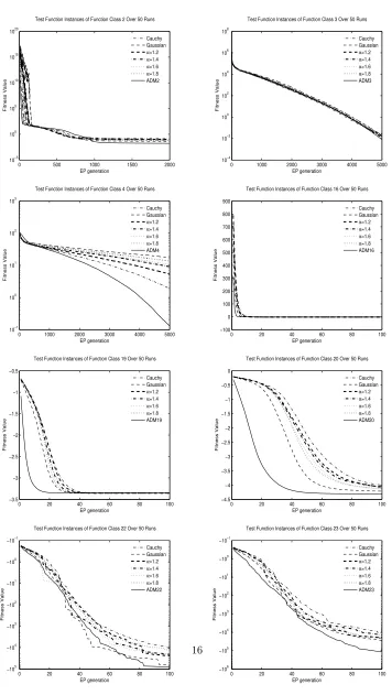
Figure 3 shows the performance of different mutation operators during an EP run, using a single

function for eight of the function classes tested.

The ADMs show significant improvement on f2, f3, f4, f20, f22, f23. The figures of f4, f19,

f20 and f23 shows that the ADMs not only perform well in early generations of the evolutionary

process, but also in later generations. The figure forf2shows that ADM2 has good performance in

the early generations, poor performance towards the middle, but outperforms all other methods by

the end the run. This phenomenon was also found and discussed in previous references combining

Cauchy and Gaussian mutation operators together. This suggests that, as the performance of a

mutation operators varies at different stages of the search, using dynamic or multiple mutation

operators may be preferable to using a single operator.

5.1. Performance of Evolved Mutation Operators on Other Function Classes

As a result of the train-and-test approach used, each ADM evolved by GP is designed for a

specific function class. For example, ADM1 was designed for functions drawn from the function

class f1. Specifically, it was trained on 10 functions (although only 5 were used for evaluation)

drawn fromf1and tested on a further 50 functions also taken from f1. This presents the following

0 500 1000 1500 2000 10−5 100 105 1010 1015 1020 EP generation Fitness Value

Test Function Instances of Function Class 2 Over 50 Runs

Cauchy Gaussian α=1.2 α=1.4 α=1.6 α=1.8 ADM2

0 1000 2000 3000 4000 5000

10−4 10−2 100 102 104 106 108 EP generation Fitness Value

Test Function Instances of Function Class 3 Over 50 Runs

Cauchy Gaussian α=1.2 α=1.4 α=1.6 α=1.8 ADM3

0 1000 2000 3000 4000 5000

10−1 100 101 102 103 EP generation Fitness Value

Test Function Instances of Function Class 4 Over 50 Runs

Cauchy Gaussian α=1.2 α=1.4 α=1.6 α=1.8 ADM4

0 20 40 60 80 100

−100 0 100 200 300 400 500 600 700 800 900 EP generation Fitness Value

Test Function Instances of Function Class 16 Over 50 Runs

Cauchy Gaussian α=1.2 α=1.4 α=1.6 α=1.8 ADM16

0 20 40 60 80 100 −3.5 −3 −2.5 −2 −1.5 −1 −0.5 EP generation Fitness Value

Test Function Instances of Function Class 19 Over 50 Runs

Cauchy Gaussian α=1.2 α=1.4 α=1.6 α=1.8 ADM19

0 20 40 60 80 100

−4.5 −4 −3.5 −3 −2.5 −2 −1.5 −1 −0.5 0 EP generation Fitness Value

Test Function Instances of Function Class 20 Over 50 Runs

Cauchy Gaussian α=1.2 α=1.4 α=1.6 α=1.8 ADM20

0 20 40 60 80 100

−105 −104 −103 −102 −101 −100 −10−1 EP generation Fitness Value

Test Function Instances of Function Class 22 Over 50 Runs

Cauchy Gaussian α=1.2 α=1.4 α=1.6 α=1.8 ADM22

0 20 40 60 80 100

−106 −105 −104 −103 −102 −101 −100 −10−1 EP generation Fitness Value

Test Function Instances of Function Class 23 Over 50 Runs

from a different function class? In other words, is the tailored ADM better than an arbitrary ADM?

We will now compare the performance of an ADM tailored to one function class with the other

22 ADMs which are intended for use on different function classes. The mean values and standard

deviations achieved by each ADM are presented in Tables 8 and 9. The diagonal is in boldface

and represents the performance of ADMion the function classfi. For a given row (fi), the values

in boldface indicate the ADMs that have beaten ADMi on fi. For example, for f1, ADM1 is

outperformed only by ADM10. From both tables we can see that ADM8, ADM11, ADM12 and

ADM16 have the best performance on f8, f11, f12 andf16, respectively. ADM1, ADM4, ADM7,

ADM9, ADM13, ADM19 and ADM20 have the second best performance on f1, f4, f7, f9, f13,

f19 andf20, respectively. The worst performance of the tailored ADMs are ADM15, ADM18 and

ADM22: their ranks are 11th, 11th, and 12th, onf15,f18andf22, respectively. Overall, as expected

an ADM tailored to a function class has better performance than the non-tailored ADMs. Table 10

shows the results of a Wilcoxon signed-rank test within a 95% confidence interval of a tailored ADM

(TADM) compared with non-tailored ADMs (with statistically significant differences in boldface).

The tailored ADM is an ADM trained for that specific function class. For example, ADM1 is the

TADM for function class 1, but ADM1 is a non-tailored ADM for function class 2. In this table,

‘≥’ and ‘≤’ indicate that an ADM performs better or worse than the other ADMs. In the case that

this difference is statistically significant, ‘>’ and ‘<’ are used. Although ADM16 shows the best

performance on f16, in Table 10 ‘=’ indicates that the performances of ADM16 and ADM19 are

equal onf16. Forf8, ‘≥’ indicates that the performance of ADM8 is better than that of ADM23,

but that this is not significant. As can be seen from the last column in Table 10, in the majority of

Table 8: Comparison (averaged over 20 runs) of each of the 23 ADMs on each of the 23 function classes (f1–f19). The fitness value of the TADM is in bold, and those other fitness values that are better than the fitness value of the TADM are also in bold.

ADM1 ADM2 ADM3 ADM4 ADM5 ADM6 ADM7 ADM8 ADM9 ADM10 ADM11 ADM12 ADM13 ADM14 ADM15 ADM16 ADM17 ADM18 ADM19 ADM20 ADM21 ADM22 ADM23

f1

3.79604 3.79679 3.79617 3.80010 3.79822 3.79843 3.79682 2531.21 3.79606 3.79599 3.84599 3.79619 3.79628 3.79665 3.79612 1655.31 16670.68 3.80282 4.26045 3.79609 44.19 3.79607 3.81683

(15.53) (15.53) (15.53) (15.53) (15.53) (15.53) (15.53) (11290.26) (15.53) (15.53) (15.53) (15.53) (15.53) (15.53) (15.53) (2395.68) (7873.98) (15.53) (15.51) (15.53) (49.93) (15.53) (15.53)

f2

3.27E-02 1.73E-02 6.41E-02 2.44E-01 2.27E-01 2.42E-01 1.41E-01 10.89 1.26E-02 1.56E-02 8.78E-01 4.83E-02 6.82E-02 1.02E-01 3.30E-02 5.65 62.09 2.94E-02 3.08E-03 8.14E-03 2.69E-01 3.31E-02 3.96E-02

(6.2E-03) (3.2E-03) (1.2E-02) (5.3E-02) (4.2E-02) (4.5E-02) (2.7E-02) (29.6) (2.4E-03) (3.2E-03) (2.2E-01) (9.0E-03) (1.3E-02) (2.1E-02) (6.5E-03) (6.57) (15.77) (5.4E-03) (8.5E-04) (1.5E-03) (1.5E-01) (6.5E-03) (3.9E-02)

f3

0.0591 0.5426 0.0186 0.1031 0.0139 0.0142 0.0059 33.78 2.67 2.04 0.9379 0.2866 0.0641 0.0970 0.0849 3433.71 7087.02 0.1574 50.23 5.58 11.02 0.1992 182.15 (0.1276) (0.9071) (0.0388) (0.0522) (0.0062) (0.0059) (0.0031) (25.61) (3.03) (2.68) (0.4713) (0.4207) (0.1000) (0.1135) (0.1233) (3872.31) (4298.40) (0.1946) (47.12) (6.89) (7.78) (0.3809) (157.13)

f4

17.26 19.42 16.15 0.29 9.65 14.05 16.79 28.13 10.99 14.20 0.16 2.63 4.40 1.33 21.58 68.40 74.66 40.88 37.07 16.70 61.05 15.81 8.93 (4.97) (7.25) (4.89) (0.50) (5.40) (7.01) (7.26) (43.09) (5.90) (6.77) (0.13) (2.04) (2.85) (1.70) (7.95) (7.99) (7.26) (9.61) (14.01) (5.75) (8.86) (4.98) (5.60)

f5

-12.5987 -11.3929 -13.3862 -12.1777 -12.9862 -13.2639 -13.4344 4522608.39 -12.8065 -12.3842 -10.2108 -12.6180 -12.0733 -12.3406 -11.3735 768.5564 189434.0968 -11.6838 -10.2007 -10.9133 6.0180 -12.7928 -7.3536 (19.08) (16.78) (19.29) (20.18) (18.94) (19.31) (19.83) (4559249.52)(19.39) (17.83) (18.26) (18.51) (17.93) (17.08) (18.02) (1491.14) (135909.77) (18.82) (17.38) (18.05) (25.80) (19.30) (20.10)

f6

422.03 1143.00 12.17 0.135 0.058 0.054 0.11 9.298 0.107 0.015 0.326 0.039 0.035 0.032 195.78 17987.88 37431.70 424.44 375.22 0.017 4999.89 185.43 83.99 (1649.47) (2074.28) (38.35) (0.27) (0.22) (0.22) (0.30) (6.86) (0.25) (0.02) (0.16) (0.06) (0.07) (0.02) (490.12) (13480.82) (19447.52) (752.32) (888.00) (0.03) (5268.86) (446.24) (123.80)

f7

0.0655 0.0783 0.0562 0.0841 0.0470 0.0488 0.0487 2.8072 0.0635 0.0586 0.1949 0.0619 0.0537 0.0623 0.0702 0.5328 45.5222 0.0915 0.0870 0.0659 0.4786 0.0629 0.1865 (0.0108) (0.0243) (0.0116) (0.0196) (0.0061) (0.0065) (0.0077) (1.2139) (0.0128) (0.0093) (0.0418) (0.0107) (0.0081) (0.0107) (0.0105) (0.4611) (19.5016) (0.0228) (0.0255) (0.0123) (0.1751) (0.0157) (0.1112)

f8

-7476.80 -7873.51 -8371.09 -11531.08 -8638.19 -8567.79 -8461.85 -12471.54 -10836.76 -10864.24 -11921.11 -11261.25 -11017.46 -11363.52 -7712.38 -9103.97 -7289.48 -7716.48 -11715.12 -10802.04 -7922.38 -8271.94 -12347.43 (648.37) (503.11) (779.63) (307.06) (533.70) (489.80) (682.14) (158.44) (498.97) (528.49) (319.68) (332.98) (352.28) (396.68) (673.42) (629.07) (588.01) (519.33) (392.40) (383.83) (534.77) (686.29) (208.99)

f9

-6.3643 -6.6138 -7.2742 -8.8411 -6.5252 -6.6248 -6.1178 -7.4905 -8.8540 -8.8540 -8.7243 -8.8536 -8.8532 -8.8521 -5.7131 -8.4279 11.8005 -6.4276 -8.7550 -8.8541 -5.8654 -7.2526 -8.8323 (13.55) (14.20) (13.11) (11.28) (13.91) (14.12) (14.37) (11.30) (11.28) (11.28) (11.25) (11.28) (11.28) (11.28) (15.25) (11.22) (19.67) (13.48) (11.37) (11.28) (13.78) (13.43) (11.26)

f10

-26.5488 -27.6246 -27.8734 -28.5297 -28.4378 -27.4749 -28.1247 -7.2537 -28.5828 -28.5820 -23.8488 -28.5745 -28.5713 -28.5635 -27.3001 -16.8669 -4.3441 -26.5893 -28.4834 -28.5836 -23.4200 -27.4131 -28.5401 (8.64) (7.69) (7.11) (6.28) (6.45) (8.12) (6.63) (14.71) (6.29) (6.29) (13.26) (6.29) (6.29) (6.29) (7.78) (9.53) (2.23) (8.95) (6.39) (6.29) (9.54) (7.76) (6.29)

f11

-0.6511 -0.4304 -0.6994 -0.7322 -0.6968 -0.7229 -0.6814 -0.7159 -0.6402 -0.6742 -0.7384 -0.7172 -0.7353 -0.7251 -0.6194 72.6735 245.0964 -0.3781 -0.3158 -0.5856 5.0014 -0.5955 -0.7322 (0.55) (0.59) (0.53) (0.55) (0.57) (0.54) (0.55) (0.55) (0.56) (0.55) (0.55) (0.56) (0.54) (0.54) (0.53) (74.08) (108.70) (0.52) (0.64) (0.54) (4.93) (0.54) (0.55)

f12

2.38 1.52 8.18E-01 4.99E-05 1.14 1.08 2.61 2.95E+08 8.63E-02 4.90E-02 7.61E-04 2.74E-06 2.39E-02 9.89E-06 1.50 34.73 1.5E+07 2.15 2.01E-01 1.21E-01 18.16 1.13 4.26E+04 (2.85) (2.15) (1.30) (1.32E-05) (1.20) (2.17) (3.63) (5.62E+08) (2.99E-01) (1.77E-01) (2.36E-04) (1.09E-06) (5.98E-02) (3.88E-06) (1.33) (35.79) (2.46E+07) (1.76) (4.23E-01) (3.22E-01) (10.06) (1.06) (1.90E+05)

f13

7.53 11.54 5.38 6.69E-04 3.18 5.34 10.81 4.51E+08 3.80E-03 1.87E-03 1.01E-02 4.50E-05 6.35E-05 1.26E-04 3.66 333.02 7.36E+06 18.23 7.15E-01 2.86E-02 257.29 5.85 527.92 (11.5) (12.6) (10.3) (1.4E-04) (5.0) (5.6) (19.7) (611339756.7)(7.1E-03) (4.6E-03) (2.3E-03) (2.0E-05) (1.7E-05) (2.9E-05) (4.6) (304.3) (4.79E+06) (21.7) (1.6) (7.2E-02) (118.6) (7.5) (2359.9)

f14

1.73 1.77 1.23 1.07 1.69 1.81 1.17 0.75 1.29 1.05 0.78 0.83 1.24 0.84 1.46 2.63 0.99 1.35 1.25 1.65 1.54 1.05 0.87 (1.39) (1.52) (0.56) (0.66) (1.66) (1.35) (0.60) (0.17) (1.08) (0.57) (0.17) (0.31) (1.22) (0.34) (0.86) (3.71) (0.55) (0.87) (1.99) (1.30) (1.42) (0.68) (0.35)

f15

6.43E-04 1.55E-03 7.85E-04 7.66E-04 2.25E-03 1.92E-03 1.20E-03 1.64E-03 5.36E-04 4.18E-04 1.10E-03 5.80E-04 5.80E-04 6.34E-04 7.07E-04 1.55E-03 1.23E-03 1.41E-03 4.96E-04 4.42E-04 6.56E-04 4.79E-04 8.71E-04 (5.4E-04) (4.4E-03) (8.6E-04) (8.6E-04) (5.8E-03) (3.5E-03) (1.8E-03) (2.0E-03) (3.7E-04) (2.9E-04) (1.2E-03) (4.0E-04) (3.6E-04) (3.9E-04) (5.4E-04) (4.5E-03) (6.9E-06) (3.9E-03) (3.9E-04) (3.5E-04) (4.3E-04) (3.1E-04) (4.5E-04)

f₁₆

-1.92447213 -1.924473263-1.924470875-1.924468207-1.924439114-1.924429001-1.924455664-1.924280681-1.924473516-1.924473529-1.924454275-1.924473348-1.924472904-1.924472224-1.924472113-1.924473543-1.92447336 -1.924472505-1.924473543-1.924473528-1.924473215-1.924473016-1.92447352 (0.58) (0.58) (0.58) (0.58) (0.58) (0.58) (0.58) (0.58) (0.58) (0.58) (0.58) (0.58) (0.58) (0.58) (0.58) (0.58) (0.58) (0.58) (0.58) (0.58) (0.58) (0.58) (0.58)

f₁₇

3.786952682 3.786952414 3.786953089 3.786953821 3.786960153 3.786965855 3.786956682 3.7870070253.786952351 3.7869523473.78696211 3.786952403 3.78695256 3.786952596 3.7869526883.786952342 3.7869523953.78695256 3.7869532073.7869523463.786952426 3.786952433 3.786952348 (2.37) (2.37) (2.37) (2.37) (2.37) (2.37) (2.37) (2.37) (2.37) (2.37) (2.37) (2.37) (2.37) (2.37) (2.37) (2.37) (2.37) (2.37) (2.37) (2.37) (2.37) (2.37) (2.37)

f₁₈

4.5750315334.5749718194.575098811 4.575282035 4.5763558 4.577539016 4.575858015 4.5887151334.574958404 4.5749582054.5763717224.5749678134.575001205 4.575011001 4.575028689 6.0057613374.574969199 4.575008958 4.57495705 4.574957813 4.574974777 4.574979692 4.57495876 (1.12) (1.12) (1.12) (1.12) (1.12) (1.12) (1.12) (1.11) (1.12) (1.12) (1.12) (1.12) (1.12) (1.12) (1.12) (6.14) (1.12) (1.12) (1.12) (1.12) (1.12) (1.12) (1.12)

Table 9:Comparison (averaged over 20 runs) of each of the 23 ADMs on each of the 23 function classes (f20–f23).

ADM1 ADM2 ADM3 ADM4 ADM5 ADM6 ADM7 ADM8 ADM9 ADM10 ADM11 ADM12 ADM13 ADM14 ADM15 ADM16 ADM17 ADM18 ADM19 ADM20 ADM21 ADM22 ADM23

f20

-4.0774 -4.0748 -3.8878 -4.0932 -4.0110 -3.4181 -4.0560 -3.9522 -4.1095 -4.1141 -3.8083 -4.1051 -4.1100 -3.8682 -4.0393 -4.0958 -4.0869 -4.0615 -4.1102 -4.1107 -4.0990 -4.0948 -4.1099

(2.02) (1.98) (1.95) (2.02) (2.10) (1.85) (2.03) (2.02) (2.04) (2.04) (1.97) (2.05) (2.04) (1.85) (2.07) (2.05) (1.99) (1.98) (2.05) (2.04) (2.05) (2.02) (2.04)

f21

-7.50 -8.26 -6.75 -3.69 -4.44 -4.58 -4.06 -3.64 -7.63 -7.12 -3.55 -7.50 -7.12 -5.96 -7.50 -3.99 -8.24 -6.87 -3.97 -8.14 -7.63 -7.24 -6.99

(2.4) (1.6) (2.9) (1.5) (1.9) (2.6) (1.7) (0.3) (2.3) (2.7) (0.7) (2.3) (2.7) (2.6) (2.1) (3.3) (1.5) (2.7) (2.7) (1.9) (2.4) (2.3) (2.5)

f22

-22690.01 -138764.16 -16262.26 -7564.46 -4081.24 -7710.71 -8391.89 -661.13 -138490.10 -156034.53 -2163.99 -121815.79 -75620.18 -21671.31 -184449.89 -20512221.26-71248.07 -53103.24 -3872071.64 -266869.50 -88299.30 -72258.79 -156292.70

(30957.5) (240207.8) (22759.7) (14484.9) (7046.2) (20971.9) (15850.7) (1197.4) (193997.9) (256068.3) (4065.4) (272880.3) (142754.5) (34334.5) (574931.9) (81568165.2)(109512.0) (85281.3) (7903902.6) (408822.5) (146589.9) (79909.2) (227462.4)

f23

-32152.70 -52174.33 -26607.57 -21922.82 -6153.03 -5790.76 -9617.22 -380.46 -103530.92 -132236.20 -2388.34 -50209.17 -29264.20 -14424.39 -24997.68 -3511793.67-98707.40 -211246.70 -1024445.84 -290292.30 -107802.76 -36810.44 -111941.27 (61337.3) (93572.1) (68340.3) (54964.3) (11938.5) (11424.6) (19983.7) (657.0) (206684.0) (244626.7) (4202.0) (100548.3) (59321.4) (31387.8) (51026.8) (8105197.0) (235422.7) (642660.0) (2471291.7) (839727.1) (284455.3) (74288.9) (233075.7)

Table 10: Comparison of ADMs on different function classes.

FC TADM TADM TADM TADM TADM TADM TADM TADM TADM TADM TADM TADM TADM TADM TADM TADM TADM TADM TADM TADM TADM TADM TADM TADM WIN -ADM1 -ADM2 -ADM3 -ADM4 -ADM5 -ADM6 -ADM7 -ADM8 -ADM9 -ADM10 -ADM11 -ADM12 -ADM13 -ADM14 -ADM15 -ADM16 -ADM17 -ADM18 -ADM19 -ADM20 -ADM21 -ADM22 -ADM23 TIMES

f1 N/A > > > > > > > ≥ < > > > > ≥ > > > > ≥ > ≥ > 21

f2 > N/A > > > > > > < < > > > > > > > > < < > > > 18

f3 ≥ > N/A > ≤ ≤ ≤ > > > > > > > > > > > > > > > > 19

f4 > > > N/A > > > > > > ≤ > > > > > > > > > > > > 21

f5 ≥ ≥ ≤ ≥ N/A ≤ ≤ > ≥ ≥ > ≥ ≥ ≥ > > > ≥ > > > ≥ > 19

f6 > > > > ≥ N/A ≥ > > ≤ > < < < > > > > > ≤ > > > 17

f7 > > > > ≤ ≥ N/A > > > > > > > > > > > > > > > > 21

f₈ > > > > > > > N/A > > > > > > > > > > > > > > ≥ 22

f9 > > > > > > > > N/A > > > > > > ≥ > > > < > > > 21

f10 > ≥ > > > > > > < N/A > > > > > > > > > < > > > 20

f₁₁ > > > ≥ > ≥ > > > > N/A > ≥ > > > > > > > > > > 22

f12 > > > > > > > > > ≥ > N/A > > > > > > > > > > > 22

f13 > > > > > > > > > ≥ > < N/A > > > > > > > > > > 21

f₁₄ > > > ≥ > > ≥ ≤ ≥ ≥ ≤ ≤ ≥ N/A > > ≥ > ≥ ≥ ≥ ≥ ≥ 19

f15 ≤ ≥ ≥ ≥ ≥ > > > < < > ≤ ≥ ≤ N/A > > ≥ < < ≤ < ≥ 12

f16 > > > > > > > > > > > > > > > N/A > > = > > > > 22

f₁₇ > ≥ > > > > > > < < > ≥ > > > < N/A > > < > ≥ > 18

f18 > < > > > > > > < < > < ≥ ≥ > > < N/A < < < < < 12

f19 > > > > > > > > > > > > > > > ≤ > > N/A > > > > 21

f₂₀ > > > > > > > > > < > > > > > ≥ > > ≥ N/A > > > 21

f21 ≥ < > > > > > > ≥ ≥ > ≥ ≥ > ≥ > ≤ ≥ > ≤ N/A ≥ ≥ 19

f22 > ≤ > > > > > > < ≤ > ≤ ≤ > ≤ ≤ ≥ ≥ ≤ < ≤ N/A ≤ 11

f₂₃ ≥ ≥ ≥ ≥ ≥ > > > ≥ ≤ > ≥ > ≥ ≥ ≤ ≥ ≤ ≤ ≤ ≥ ≥ N/A 17

6. Discussion

One of the advantages of the new method presented here is that it eliminates the need for human

researchers to continually propose new distributions for use as mutation operators in EP. Instead, we

have a search space which contains a rich set of mutation operators, and we can let a metaheuristic,

such as GP, sample this space and select a suitable choice for the sample of functions at hand.

In addition, it designs an ADM within the context of a function class. In other words, it tailors

a mutation operator (random number generator) to a function class (probability distribution over

functions). The suitability of mutation operator depends on the function class. Rather than tuning

anumerical parameter to a function class, it tunes aprogram that generates random numbers to a

function class.

One of the apparent disadvantages of the proposed system is the time needed to evolve the

ADMs. This is because we have an EP algorithm at the base level, the mutation operator of

which is being evolved by a GP algorithm at the hyper-level. While this may appear to be a

superficial disadvantage, there are other advantages. Firstly, it is difficult to measure the amount

of human effort required in designing a new mutation operator, and therefore it is difficult to directly

compare the design phases of human and machine (GP in this case). We can only sensibly compare

the performance of two mutation operators at the testing phase. Secondly, the system can be used

to automatically generate new ADMs as and when needed to the demands of a new function class,

whereas the human designer would have to start the whole process over again.

It is important to note that the fact that the training and testing are drawn from the same

distribution is central to the train-and-test approach. In our case, this means that an ADM is

developed to be used as a mutation operator for a given function class, but also, importantly,

within a given EP algorithm, which includes a fixed EP population size and number of generations.

One of the current limitations of the proposed method is that not only must the training set

of functions be representative of the testing set of functions, but also the conditions under which

they are sampled must be similar. For example, when testing a function from function classf1, we

used the same population size and number of generations of EP as in the training phase. This is

a limitation which needs to be addressed. One possibility would be to use GP to train EP using a

different number of generations and population sizes. However, this would only partially address

the issue, since if we attempted to use an ADM with a population size and number of generations

7. Summary and Future Work

In this paper we have used genetic programming (GP) as an offline hyper-heuristic to

automat-ically evolve probability distributions, to use as mutation operators in evolutionary programming

(EP). This is in contrast to existing operators in the literature which are human designed. The

function and terminal set for GP was chosen to be able to express a number of currently existing

human designed mutation operators, namely Cauchy, Gaussian and L´evy, and also express novel

automatically designed mutation operators (ADMs). Each ADM is constructed from a function set

including arithmetic and trigonometric functions, and a terminal set of probability distributions

included as standard in many programming libraries and mathematical packages. Using a

train-and-test approach, where two independent sets of functions are drawn from the samefunction class

for training and testing, it is shown that GP is capable of generating ADMs which outperform

existing EP variants over a number of different function classes. As an additional validation

exer-cise, we have also presented experiments to show that the ADM tailored to a given function class

performs better that ADMs tailored to different function classes.

There are a number of possible directions for future work. As GP has been able to evolve good

variation operators for EP, further work will explore the ability of GP to generate variation operators

for other real-valued optimisation methods such as differential evolution (DE) and particle swarm

optimisation (PSO), particularly for the case of function classes where a train-and-test approach

can be used. Another direction within EP is to extend our hyper-heuristic approach beyond simple

static mutation operators. It has been observed previously that both Cauchy and Gaussian mutation

are effective in EP at different points of a search [35]. As both of these operators can be defined

as a parameterised version of the L´evy distribution, through the use of differentαvalues, we will

evolve the value ofαas a function over time, subsequently defining a family of adaptive mutation

operators which can be trained to specialise in solving different classes of functions.

References

[1] X. Yao, Y. Liu, Fast evolutionary programming, in: Proceedings of the Fifth Annual Conference

on Evolutionary Programming, MIT Press, 1996, pp. 451–460.

[2] N. Sinha, R. Chakrabarti, P. Chattopadhyay, Evolutionary programming techniques for

[3] P. Shelokar, A. Quirin, O. Cord´on, A multiobjective evolutionary programming framework for

graph-based data mining, Information Sciences 237 (2013) 118–136.

[4] M. Mutyalarao, A. Sabarinath, M. Xavier James Raj, Taboo evolutionary programming

ap-proach to optimal transfer from earth to mars, in: Proceedings of Swarm, Evolutionary, and

Memetic Computing (SEMCCO 2011) - Part II, Vol. 7077 of LNCS, Springer, Visakhapatnam,

Andhra Pradesh, India, 2011, pp. 122–131.

[5] A. K. Qin, V. L. Huang, P. N. Suganthan, Differential evolution algorithm with strategy

adaptation for global numerical optimization, IEEE transactions on Evolutionary Computation

13 (2) (2009) 398–417.

[6] R. Mallipeddi, P. N. Suganthan, Q.-K. Pan, M. F. Tasgetiren, Differential evolution algorithm

with ensemble of parameters and mutation strategies, Applied Soft Computing 11 (2) (2011)

1679–1696.

[7] J. Kennedy, R. Eberhart, Particle swarm optimization, in: Proceedings of the IEEE

Interna-tional Conference on Neural Networks, Vol. 4, Perth, Australia, 1995, pp. 1942–1948.

[8] N. Hansen, The cma evolution strategy: A comparing review, in: Towards a New Evolutionary

Computation, Vol. 192 of Studies in Fuzziness and Soft Computing, Springer Berlin Heidelberg,

2006, pp. 75–102.

[9] S. M. Elsayed, R. A. Sarker, D. L. Essam, Adaptive configuration of evolutionary algorithms

for constrained optimization, Applied Mathematics and Computation 222 (2013) 680–711.

[10] E. Burke, M. Hyde, G. Kendall, G. Ochoa, E. ¨Ozcan, J. Woodward, A classification of

hyper-heuristic approaches, in: M. Gendreau, J.-Y. Potvin (Eds.), Handbook of Metahyper-heuristics, Vol.

146 of International Series in Operations Research and Management Science, Springer US,

2010, pp. 449–468.

[11] R. Poli, W. B. Langdon, N. F. McPhee, A field guide to genetic programming, Published via

http://lulu.com and freely available at http://www.gp-field-guide.org.uk, 2008, (With

contri-butions by J. R. Koza).

[12] E. Burke, M. Hyde, G. Kendall, G. Ochoa, E. ¨Ozcan, J. Woodward, Exploring hyper-heuristic

Intelligence, Vol. 1 of Intelligent Systems Reference Library, Springer Berlin Heidelberg, 2009,

pp. 177–201.

[13] J. R. Woodward, J. Swan, Automatically designing selection heuristics, in: Proceedings of

the Genetic and Evolutionary Computation Conference Companion (GECCO 2011), ACM,

Dublin, Ireland, 2011, pp. 583–590.

[14] J. R. Woodward, J. Swan, The automatic generation of mutation operators for genetic

algo-rithms, in: Proceedings of the Genetic and Evolutionary Computation Conference Companion

(GECCO 2012), ACM, Philadelphia, Pennsylvania, USA, 2012, pp. 67–74.

[15] L. Dio¸san, M. Oltean, Evolving crossover operators for function optimization, in: P. Collet,

M. Tomassini, M. Ebner, S. Gustafson, A. Ek´art (Eds.), Proceedings of the European

Con-ference on Genetic Programming (EuroGP 2006), Vol. 3905 of LNCS, Springer, Budapest,

Hungary, 2006, pp. 97–108.

[16] S. Nguyen, M. Zhang, M. Johnston, K. Tan, Automatic design of scheduling policies for

dy-namic multi-objective job shop scheduling via cooperative coevolution genetic programming,

IEEE Transactions on Evolutionary Computation 18 (2) (2013) 193–208.

[17] R. E. Keller, R. Poli, Linear genetic programming of parsimonious metaheuristics, in: D.

Srini-vasan, L. Wang (Eds.), Proceedings of the IEEE Congress on Evolutionary Computation (CEC

2007), IEEE Press, Singapore, 2007, pp. 4508–4515.

[18] M. Bader El Den, R. Poli, Grammar-based genetic programming for timetabling, in:

Proceed-ings of the IEEE Congress on Evolutionary Computation (CEC 2009), IEEE Press, Piscataway,

NJ, USA, 2009, pp. 2532–2539.

[19] M. Bader El Den, R. Poli, S. Fatima, Evolving timetabling heuristics using a grammar-based

genetic programming hyper-heuristic framework, Memetic Computing 1 (3) (2009) 205–219.

[20] J. H. Drake, M. Hyde, K. Ibrahim, E. ¨Ozcan, A genetic programming hyper-heuristic for the

multidimensional knapsack problem, Kybernetes 43 (9-10) (2014) 1500–1511.

[21] L. Hong, J. Woodward, J. Li, E. ¨Ozcan, Automated design of probability distributions as

mutation operators for evolutionary programming using genetic programming, in: Genetic

[22] G. L. Pappa, A. A. Freitas, Discovering new rule induction algorithms with grammar-based

genetic programming, in: Soft Computing for Knowledge Discovery and Data Mining, Springer,

2008, pp. 133–152.

[23] S. Nguyen, M. Zhang, M. Johnston, K. C. Tan, Automatic design of scheduling policies for

dynamic multi-objective job shop scheduling via cooperative coevolution genetic programming,

IEEE Transactions on Evolutionary Computation 18 (2) (2014) 193–208.

[24] J. Park, S. Nguyen, M. Zhang, M. Johnston, Evolving ensembles of dispatching rules using

genetic programming for job shop scheduling, in: Genetic Programming, Vol. 9025 of Lecture

Notes in Computer Science, Springer International Publishing, 2015, pp. 92–104.

[25] J. Branke, S. Nguyen, C. W. Pickardt, M. Zhang, Automated design of production scheduling

heuristics: A review, IEEE Transactions on Evolutionary Computation 20 (1) (2016) 110–124.

[26] R. Poli, J. Woodward, E. K. Burke, A histogram-matching approach to the evolution of

bin-packing strategies., in: Proceedings of the IEEE Congress on Evolutionary Computation (CEC

2007), IEEE, 2007, pp. 3500–3507.

[27] E. K. Burke, M. R. Hyde, G. Kendall, J. Woodward, Automatic heuristic generation with

genetic programming: evolving a jack-of-all-trades or a master of one, in: Proceedings of

the Genetic and Evolutionary Computation Conference Companion (GECCO 2007), ACM,

London, England, 2007, pp. 1559–1565.

[28] E. K. Burke, M. R. Hyde, G. Kendall, J. R. Woodward, The scalability of evolved on line bin

packing heuristics, in: D. Srinivasan, L. Wang (Eds.), Proceedings of the IEEE Congress on

Evolutionary Computation (CEC 2007), IEEE Press, Singapore, 2007, pp. 2530–2537.

[29] A. Parkes, E. ¨Ozcan, M. Hyde, Matrix analysis of genetic programming mutation, in:

A. Moraglio, S. Silva, K. Krawiec, P. Machado, C. Cotta (Eds.), Genetic Programming, Vol.

7244 of LNCS, Springer Berlin Heidelberg, 2012, pp. 158–169.

[30] E. ¨Ozcan, A. J. Parkes, Policy matrix evolution for generation of heuristics, in: Proceedings of

the Genetic and Evolutionary Computation Conference (GECCO 2011), ACM, Dublin, Ireland,

[31] J. H. Drake, J. Swan, G. Neumann, E. ¨Ozcan, Sparse, continuous policy representations for

uniform online bin packing via regression of interpolants, in: European Conference on

Evo-lutionary Computation in Combinatorial Optimization (EvoCOP 2017), Vol. 10197 of LNCS,

Springer, 2017, pp. 189–200.

[32] R. Poli, W. Langdon, O. Holland, Extending particle swarm optimisation via genetic

pro-gramming, in: M. Keijzer, A. Tettamanzi, P. Collet, J. Hemert, M. Tomassini (Eds.), Genetic

Programming, Vol. 3447 of LNCS, Springer Berlin Heidelberg, 2005, pp. 291–300.

[33] J. Drake, N. Kililis, E. ¨Ozcan, Generation of vns components with grammatical evolution for

vehicle routing, in: Genetic Programming, Vol. 7831 of LNCS, Springer Berlin Heidelberg,

2013, pp. 25–36.

[34] L. Hong, J. H. Drake, J. R. Woodward, E. ¨Ozcan, Automatically designing more general

mutation operators of evolutionary programming for groups of function classes using a

hyper-heuristic, in: Proceedings of the Genetic and Evolutionary Computation Conference (GECCO

2016), ACM, New York, NY, USA, 2016, pp. 725–732.

[35] X. Yao, Y. Liu, G. Lin, Evolutionary programming made faster, IEEE Transactions on

Evolu-tionary Computation 3 (1999) 82–102.

[36] T. B¨ack, H.-P. Schwefel, An overview of evolutionary algorithms for parameter optimization,

Evolutionary Computation 1 (1) (1993) 1–23.

[37] C.-Y. Lee, X. Yao, Evolutionary programming using mutations based on the l´evy probability

distribution, IEEE Transactions on Evolutionary Computation 8 (1) (2004) 1–13.

[38] R. N. Mantegna, Fast, accurate algorithm for numerical simulation of l´evy stable stochastic

processes, Physical Review E 49 (1994) 4677–4683.

[39] H. Dong, J. He, H. Huang, W. Hou, Evolutionary programming using a mixed mutation

strategy, Information Sciences 177 (1) (2007) 312 – 327.

[40] R. Mallipeddi, S. Mallipeddi, P. Suganthan, Ensemble strategies with adaptive evolutionary

[41] S. Silva, J. Almeida, Gplab-a genetic programming toolbox for matlab, in: Proceedings of the

Nordic MATLAB conference, 2003, pp. 273–278.

[42] S. Luke, L. Panait, Lexicographic parsimony pressure, in: Proceedings of the Genetic and

Evolutionary Computation Conference (GECCO 2002), Morgan Kaufmann Publishers, New