Performance modelling of fuel cell systems through Petri nets
Claudia Fecarotti, Centre for Risk and Reliability, University of Nottingham
John Andrews, Centre for Risk and Reliability, University of Nottingham
Key Words: Fuel cell system; System lifetime; Simulation; Petri nets.
SUMMARY & CONCLUSIONS
This paper introduces a model based on the Petri net method for the performance evaluation of fuel cell systems during operation. The model simulates the operation of the fuel cell stack and its supporting systems by taking into account the causal relationships between the operation of the balance of plant and the fuel cell stack performance. Failures of the supporting system affect the operating parameters such as the stack temperature and humidity, the reactants’ flow and pressure, and, in turn, the stack performance in terms of output voltage. Voltage degradation rates are needed in order to evaluate the system lifetime. The voltage degradation is related to the important operating parameters by means of empirical relationships. In order to demonstrate the capability of the model, numerical simulations are performed using data for voltage degradation rates collected from the literature. The voltage decay rate is modelled as a random variable within the aforementioned ranges. Time to failure and time to repair of components are generated from stochastic distributions. The use of a stochastic approach allows taking into account data uncertainty and variability. The modelling process produces distributions of the output parameters rather than point estimates delivered by alternative methods. This enables an appreciation of the best and worst possible output lifetime as well as the expected system performance. The model can be used to support the design, operation and maintenance of fuel cell systems.
1 INTRODUCTION
Reducing carbon emission by developing innovative, high quality and highly reliable low emission power generation sources is a main aim for the energy sector worldwide. In this context hydrogen and fuel cells are promising technologies for zero-emission energy conversion and power generation. Fuel cells are electrochemical devices that convert the chemical energy of a fuel, such as hydrogen, into electrical energy by reaction with oxygen or other oxidizing agents.
As a result of the chemical reactions, electrical energy is produced along with heat and water as the only by-products. Fuel cell technologies are suited to a wide range of applications, from portable to transport and stationary systems. In order to meet the power demand for a given application, single cells are connected in series to form a stack. The stack is only the core of a wider system supporting the stack
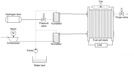
operation, referred to as the balance of plant (BOP). The BOP includes all the subsystems necessary to store and supply the reactants at the required pressure, flow rate, temperature and humidity. Those subsystems consist of pumps, control valves, blowers, pressure regulators, compressors, electric motors, intercoolers and power conditioning to regulate or convert the output voltage, and a system control. The reliability of the entire fuel cell system depends on both the reliability of the stack and the auxiliary components of the BOP. A schematic representation of a fuel cell system is given in Figure 1.
[image:1.612.317.547.310.434.2]High costs, short lifetime, durability and reliability are the main barriers to their commercialization. Quantifying the long-term performance and durability of a fuel cell is difficult because of the lack of a deep understanding of the deterioration processes occurring within the cell. Lifetime, durability and performance requirements of fuel cells stacks vary with the application. The required lifetime of fuel cells stacks range from 3000/5000 operating hours for automotive applications, up to 40,000 hours for stationary applications [1, 2]. However, the lifetime of a fuel cell stack is difficult to estimate; standard engineering measures of lifetime such as mean time to failure (MTTF) are difficult to specify since the fuel cell performance degrades gradually due to the ageing of its components and degradation rates strongly depend on the cell operating conditions. The gradual decline in voltage is usually given in units of millivolts per 1000 hours and an average degradation rate range of 1 - 10 µVh-1 over the entire lifetime is commonly accepted for most applications [1]. The fuel cell stack is considered to fail whenever it is not able to provide the required power output, either temporarily and permanently, in which case the stack needs to be replaced. The
purging of the stack is performed periodically in order to eliminate impurities and water accumulated inside the stack and therefore to restore the reversible voltage losses.
1.1 Literature review
Very little information on fuel cell systems reliability is available in the literature. In [3] Feitelberg discusses the reliability of a fleet of PEM fuel cell systems developed over a period of three years. The authors provide the most frequent causes of failure observed during operation and point out that the stack contributes to the failure more than any other component. Literature on modelling of fuel cell reliability is mainly focused on the application of fault tree analysis. Placca [4] performs a fault tree quantitative analysis listing the basic events leading to degradation of the membrane, the catalyst layers and the gas diffusion layers. Degradation rates are collected from the literature and specified for each basic event, along with the test conditions in which those degradation rates were obtained. However, the data used refers to different materials, operating conditions and test methodologies and therefore are subjected to significant uncertainty. Yousfi-Steiner et al. [5] uses fault tree analysis to gain a better understanding of PEM degradation associated with water management which strongly affects cell performance. The authors review in detail the influence of operating conditions and parameters, concluding that gas flow rate, relative humidity, temperature and current density have a major effect on water balance. Rama et al. [6] provide a structured review of the degradation processes occurring within PEM fuel cells and leading to performance losses and cell failures in the form of a failure modes and effect analysis. Although fault tree diagrams can provide a list of causes leading to cell degradation, this analysis technique is not capable to reproduce the complexity of the degradation mechanisms leading to performance loss. Degradation rates can vary drastically depending on the concurrency and combination of different operating conditions, and fault tree diagrams do not capture those dependencies between events and influencing factors. Tanrioven and Alam [7] use the Markov state-space equations to calculate the system reliability. The Weibull distribution is used to generate transition rates, while fuzzy logic is applied in order to estimate the state of health of the auxiliary components during operational lifetime. However, Markov models only account for constant transition rates.
This paper seeks to introduce an initial modelling approach based on Petri nets, for the performance analysis of fuel cell systems including the stack and the supporting system. The Petri net is a very well suited methodology to model complex systems with true concurrency and dependencies. To the best of the authors’ knowledge the only research contribution featuring the use of Petri nets for computing fuel cells reliability is given in [8]. However, while the model in [8] considers the reliability of the stack only, in the paper presented here, the boundaries of the model are extended to include the balance of the plant. The model
simulates the operation of the fuel cell stack and its supporting system to predict the system performance based on the system structure and the component’s deterioration processes. The model takes into account the causal relationships between the operation of the balance of plant (BOP) and the fuel cell stack performance. Malfunctioning and/or failures of components of the BOP affects reactants flow, stack temperature, reactants and stack humidification level, causing the stack to operate under inadequate operating conditions, with both immediate and long term effects on stack performance. The model considers the influence of those faulty operating conditions on stack voltage losses. Stochastic distributions are used to generate times when failures occur or times when threshold values for performance indicators such as fuel cells voltage are reached, given the mean time to failure of components and degradation rates. The stochastic approach also accounts for the variability of degradation rates with operating conditions.
2 PETRI NETS
Figure (2) shows a simple coloured Petri net and its marking before (a) and after (b) the transition fires. In the PN presented here, places represent the operating parameters, whose value is given by the tokens residing in the places, the state of the cells evaluated in terms of output voltage, the state of the components of the BOP. In order to provide an efficient model of the system, non-conventional transitions have been introduced. These are the “timed reset transition” and the “conditional transition”. The former has an associated list of places whose marking will be reset to an established value after the transition fires. This type of transition is used, for example, when purging is performed and part of the voltage loss is restored. A conditional transition is a stochastic transition whose firing time depends on the marking of the places connected by dashed arcs. Dashed arcs only model dependencies between the marking of the place and the firing of the connected transition, but do not imply any flow of tokens. Some transitions also perform mathematical evaluations involving the value of the input and output tokens.
Figure 3 shows the symbols used to represent the different types of transitions used in the model.
3 THE FUEL CELL SYSTEM MODEL
3.1 The balance of plant module
The balance of plant of the system at hand accounts for six main subsystems: the hydrogen supply system, the air reaction supply system, the cooling system, the reactants humidification system, the control unit and the power demand system. A basic assumption is that in normal operating conditions and steady-state operation the controllable operating parameters are kept constant. Therefore, the gas flow rate is kept constant and such to provide a stoichiometric ratio for hydrogen and reaction air of 1.2 and 2 respectively. Equally, the humidification system operates in order to humidify the gases to 100% relative humidity at 60°C. The stack unit must be provided with a continuous flow of fuel in order to sustain the power demand. Insufficient fuel supply leads to fuel starvation with consequences on both the stack output and the stack health. During operation, failure of BOP
components contributes to reduce the power output and may lead to system breakdown. The correct operation of the different parts of the engineering system directly affects the main operating parameters such as reactant flow rate and gas partial pressure, stack temperature, total pressure and water content thus influencing the stack performance. Variations in the value of the aforementioned parameters may hasten the deterioration processes occurring within the stack, thus accelerating physical degradation of components and reducing stack durability. Therefore the lifetime achievable is a trade-off between cells physical characteristics, depending on the materials used, the design and assembly of the cells and the stack, the operating conditions and the reliability of the BOP components. A Petri net model for each of the subsystems of the BOP has been developed. However in this paper only the
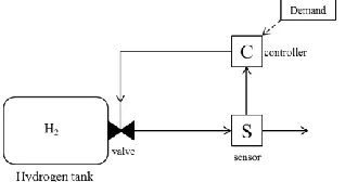
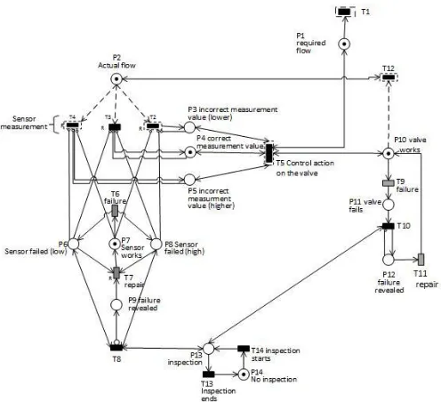
[image:3.612.49.217.37.87.2]PN for the hydrogen supply system is described for the sake of brevity (Figure 4). Hydrogen is supplied from a pressurized tank by means of a valve which regulates the flow of the inlet fuel. A sensor located after the valve, measures the flow and sends the measurement to the control unit. Based on the measured and the desired flow, the control unit sends a signal to the actuator that will set the valve to the position required in order to provide the desired hydrogen flow. Inadequate hydrogen flow supply may depend either upon a failure of the valve or a failure of the sensor. In fact, incorrect measurements prevent the control unit from setting the valve to the proper position, while a failure of the valve will prevent the actuator from changing the valve position when requested. The PN in Figure 5 represents the hydrogen supply module including both the sensor and the valve failures. Place P1 represents the demanded hydrogen flow whose value is indicated by the token. Transition T1 models changes in the flow demand and is responsible for changing the value of the token in P1. Place P2 represents the hydrogen flow rate currently provided. The hydrogen is provided by means of a valve that regulates the flow. The valve can be either in the working state, represented by place P10, or in the failed state, represented by place P11. Flow regulation is represented by transition T12 that changes the value of the token in P2 based on the position of the valve indicated by the token in place P10. When the valve is working correctly (place P10 is marked), the control unit can set the position of the valve in order to provide the required flow. Transition T5 represents the control action on the valve that depends on: (i) the valve being in the working state (P10 marked), (ii) the required flow (value of the token in P1) and (iii) the sensor measurement. The sensor, placed downstream of the valve, can either be in
[image:3.612.312.471.230.314.2]Figure 2 Marking of the PN before (a) and after (b) firing.
Figure 3 Symbols used in the PN.
[image:3.612.47.275.353.457.2]the working state, in which case place P7 is marked, or can fail. The loop P7-T6-P6-P8-T7 represents the failure and repair process for the sensor. Firing of transition T7 indicates a failure event, after which the token is moved from place P7 (working state) to either P6 or P8, representing the failed state. In the failed state the sensor can either provide a higher (place P8 is marked) or lower (place P6 is marked) measurement. Depending on the state of the sensor, the measurement provided can be correct (P4 is marked), higher (P5 is marked) or lower (P3 is marked) than the actual value. Based on the sensor measurement and the required flow, the control action, represented by T5 will set the position of the valve. During operation, the valve may fail as well. Transition T9 represents the valve failure, leading from the working state (P10 is marked) to the failed state (P11 is marked). When the valve fails, no control action can be performed on the valve, thus the hydrogen flow cannot be regulated if required (transition T5 and T12 are not enabled if P10 is not marked). In the PN the inspection process is included as well and is represented by the loop P13-T13-P14-T14. When the system is inspected place P13 is marked and failures of the sensor and the valve, if occurred, are revealed (transitions T8 and T10 may fire adding a token in places P9 and P12 respectively). Once a failure is revealed, it is assumed that a maintenance action takes place. Transitions T7 and T11 represent the repair action performed
on the sensor and the valve respectively. Once the item is repaired, the working state is considered to be restored.
3.2 The stack voltage module
Stack voltage output decreases over time as a result of aging and deterioration processes occurring within the cells. The voltage decay rate can increase severely if adverse operating conditions such as high stack temperature, low humidity levels, inadequate gases flow rates, presence of contaminants agents, fluctuating load cycles and Open Circuit
Voltage (OCV) take place. The PN for the stack voltage module is depicted in Figure 6. Place P60 represents the stack voltage above the prescribed threshold while place P59 represents the stack voltage below threshold. Transition T61 represents the degradation of stack voltage. Transition T61 fires when any change of the operating conditions causes an increase of the degradation rate. Firing of this transition will update the value of the token in P60 according to the new degradation rate. Clearly the voltage decay rate according to
which stack output voltage decreases over time depends on the particular operating circumstances represented by the marking of places P2, P16, P20, P44 , P56, P57, P58, P70. Purging is periodically performed in order to recover part of the voltage lost. The purging cycle is represented in the PN by the loop P61-T62-T63-P62-T64. When place P61 is marked, transition T62 (or alternatively T63, depending on the marking of places P59 and P60) is enabled and the firing of the transition indicates that the stack purging is taking place. Transition T64 is deterministic and its firing time depends on the frequency of purging. The voltage is treated here as a continuous variable, represented by the value of the token in place P60 (or P59 if the value is below the prescribed threshold). The voltage variation over time is approximated with a sequence of linear functions with the slope depending on the particular operating conditions.
4 MODEL ANALYSIS AND RESULTS
4.1 System specification
Values of mean time to failure (MTTF) and mean time to repair (MTTR) for the BOP components used in the simulations are detailed in Table 1.
Table 1 MTTF and MTTR of BOP components
Component MTTF (h) MTTR (h)
Sensor 2000 1 Valve 4000 1
Fan 3000 1
Pump 4000 1
[image:4.612.311.539.161.339.2]Voltage degradation rates have been collected from the
Figure 5 PN for the hydrogen supply system.
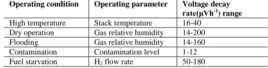
[image:4.612.51.299.346.572.2]literature [11, 12, 13, 14, 15]. Data from the literature and expert knowledge can provide the effects of operating conditions on voltage decay rate. However, based on the data collected, a ranking of the voltage decay rates based on the operating conditions and the operating parameters that showed
[image:5.612.53.298.38.211.2]a stronger impact on the voltage decay has been attempted (Table 2) and implemented within the model. Combinations of undesirable operating conditions can lead to even more severe degradation.
Table 2 Ranges of voltage decay rate for different operating conditions.
Operating condition Operating parameter Voltage decay
rate(μVh-1) range
High temperature Stack temperature 16-40 Dry operation Gas relative humidity 14-200 Flooding Gas relative humidity 14-160 Contamination Contamination level 1-12 Fuel starvation H2 flow rate 50-180
Clearly, for real applications, the characteristics of the particular fuel cell system need to be used. Under normal operating conditions (steady-state operation, Tstack=60-70°C, RH=100%) the voltage decay is assumed to vary in the range 1-10 μVh-1. It is difficult to isolate and quantify the effect of individual operating parameters in terms of the voltage
degradation rate because very often additional detrimental conditions were encountered during the tests reported in the literature. The voltage decay rate is considered here as a random variable uniformly distributed within each of the ranges detailed in Table 2. The system operation has been simulated under steady state conditions. Simulations are stopped when the voltage drops below an established threshold and is not recovered to an acceptable value (above threshold) after purging. The occurrence time of this event is considered to be the system lifetime and is recorded for each simulation along with the voltage variation over time.
4.2 Results
Convergence of results is achieved after 5000 simulations. The predicted system lifetime is recorded at the end of each simulation. Then the expected value is evaluated providing the system average lifetime. It is assumed that the stack voltage reduction is required not to exceed 0.05%. Therefore, for the 4-cell stack with initial voltage Vinit=4V, the stack voltage threshold is set to Vlim=3.8V. The lifetime values generated by the model follow a 3-parameter Weibull distribution as shown in Figure 7 with a characteristic life η= 5752, a shape parameter β= 2.7984 and a minimum life γ=1605. Figure 8 shows the unreliability function giving the chance of experiencing a failure over any specified lifetime. For instance, the probability that the system will fail within 8000 hours is approximately 0.76. The system failure rate is depicted in Figure 9 as a function of time.
The value of the shape parameter greater than 1 indicates that the fuel cell system experiences an increasing failure rate. This is due to wear-out of the stack as a consequence of ageing and degradation mechanisms. The system lifetime when different voltage threshold values are considered has been evaluated as well. The corresponding average lifetime values and the parameters of the Weibull distributions are detailed in Table 3.
Table 3Average lifetime and Weibull parameters for different
voltage thresholds. Voltage
threshold
Average lifetime
Variance Weibull parameters
3.8 6723 2048 β= 2.7984; η= 5752; γ=1605
ReliaSoft Weibull++ 7 - www.ReliaSoft.com
Unreliability vs Time Plot
Time, ( t)
U
n
re
li
a
b
il
it
y
,
F
(
t)
=
1
-R
(
t)
0.000 4000.000 8000.000 12000.000 16000.000 20000.000 0.000
1.000
0.200 0.400 0.600 0.800
Unreliability
Data 1 Weibull-3P MLE SRM MED FM F=5000/S=0
Data Points Unreliability Line
John Andrews University of Nottingham 21/10/2014 18:57:38
[image:5.612.53.301.293.467.2]Figure 7 Probability density function for Vlim=3.8V.
Figure 8 Unreliability function.
ReliaSoft Weibull++ 7 - www.ReliaSoft.com
Failure Rate vs Time Plot
Time, ( t)
F
a
il
u
re
R
a
te
,
f(
t)
/
R
(
t)
0.000 4000.000 8000.000 12000.000 16000.000 20000.000 0.000
0.003
6.000E-4 0.001 0.002 0.002
Failure Rate
Data 1 Weibull-3P MLE SRM MED FM F=5000/S=0
Failure Rate Line
[image:5.612.318.563.378.544.2]John Andrews University of Nottingham 21/10/2014 18:58:47
[image:5.612.39.306.562.630.2]3.6 9227 2403 β= 2.8846; η= 6998; γ=2986 3.4 11178 2610 β= 3.4574; η= 8781; γ=3281 3.2 12800 2886 β= 2.936; η= 8650; γ=5089 3.0 14246 3012 β= 3.5257; η= 102256; γ=5037
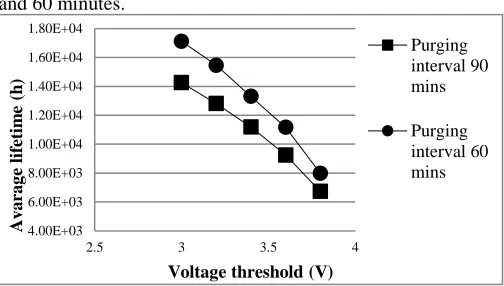
The model can be used to test different purging strategies. Figure 10 shows the average lifetime plotted against the voltage threshold for two different purging intervals of 90 and 60 minutes.
The plots show a non-linear relationship between the average lifetime and the voltage threshold. The average lifetime decreases with increasing values of the voltage threshold. It also can be observed that the system performance in terms of average lifetime increases with the frequency of purging.
5 ACKNOWLEDGEMENTS
The authors gratefully acknowledge the support of EPSRC (grant number EP/K02101X/1) which has enabled the research reported in this paper.
REFERENCES
1. S. D. Knights, K. M. Colbow, J. St-Pierre, D. P. Wilkinson. Aging mechanisms and lifetime of PEFC and DMFC. Journal of Power Sources 127 (2004) 127-134. 2. B. Belvedere, M. Bianchi, A. Borghetti, A. De Pasquale,
M. Paolone, and R. Vecci. Experimental analysis of a PEM fuel cell performance at variable load with anodic exhaust management optimization. International Journal of Hydrogen Energy, 83(2013) 385-393.
3. A. S. Feitelberg, J. Stathopoulos, Z. Qi, C. Smith and J. F. Elter. Reliability of Plug Power GenSys fuel cell systems. Journal of Power Sources 147(2005) 203-207.
4. L. Placca, R. Kouta. Fault tree analysis for PEM fuel cell degradation process modelling. International journal of hydrogen energy 36 (2011) 12393-12405.
5. N. Yousfi-Steiner, Ph. Moçotéguy, D. Candusso, D. Hissel, A.Hernandez, A. Aslanides. A review on PEM voltage degradation associated with water management: impact, influent factors and characterisation. Journal of power sources 183 (2008) 260-274.
6. P. Rama, R. Chen, J. Andrews. A review of performance
degradation and failure modes for Hydrogen-fuelled polymer electrolyte fuel cells. Proc. IMeche Vol. 222 Part A: J. Power and Energy (2008) 421-441.
7. M.Tanrioven, M.S. Alam. Reliability modelling and analysis of stand-alone PEM fuel cell power plants. Renewable Energy, Vol. 31, 2006, pp.915-933.
8. C. Wieland, O. Schmid, M. Meiler, A.Wachtel, D. Linsler. Reliability computing of polymer-electrolyte-membrane fuel cell stacks through Petri nets. Journal of Power Sources 190 (2009) 34–39.
9. T. Murata. Petri nets: properties, analysis and applications. In Proc. IEEE (1984), vol. 77, no. 4, pp. 541-580.
10. K. Jensen, L. M. Kristensen. Colored Petri nets. Modelling and validation of concurrent systems. Springer-Verlag Berlin Heidelberg 2009.
11. J. Wu, X. Z. Yuan, J.J. Martin, H. Wang, J. Zhang, J. Shen, S. Wu, W. Merida. A review of PEM fuel cell durability: Degradation mechanisms and mitigation strategies. Journal of Power Sources 184 (2008) 104–119. 12. J. Yu, T. Matsuura, Y. Yoshikawa, M. N. Islam, M. Hori. Lifetime behaviour of a PEM fuel cell with low humidification of feed stream. Phys. Chem. Chem. Phys. 7(2005) 373-378.
13. F. A. De Bruijn, V. A. T. Dam, G. J. M. Janssen. Review: durability and degradation issues of PEM fuel cell components. Fuel Cells 08, 2008, No 1, 3-22.
14. R. Mohtadi, W. Lee, J.W. van Zee. Assessing durability of cathodes exposed to common air impurities. J. Power Sources 138 (2004) 216–225.
15. J. Stumper, C. Stone. Recent advances in fuel cell technology at Ballard. J. Power Sources 176 (2008) 468– 476.
BIOGRAFIES
Claudia Fecarotti
Centre for Risk and Reliability, University Park, University of Nottingham, Nottingham, NG7 2RD, UK.
e-mail: [email protected]
Claudia Fecarotti is a Research Associate since 2013. She joined the University of Nottingham as a PhD student in 2012 after gaining her Master in Civil Engineering from the University of Palermo, Italy. Her research interests are in the area of reliability of complex engineering systems.
John Andrews
Centre for Risk and Reliability, University Park, University of Nottingham, Nottingham, NG7 2RD, UK.
e-mail: [email protected]
John Andrews holds the Royal Academy of Engineering Chair of Infrastructure Asset Management and is Director of the Lloyd’s Register Foundation Centre for Risk and Reliability Engineering. Currently active on the Safety and Reliability Group of the IMechE and Chair of the ESRA (European Safety & Reliability Association) Technical Committee for Mathematical Models in Reliability and Safety. 4.00E+03
6.00E+03 8.00E+03 1.00E+04 1.20E+04 1.40E+04 1.60E+04 1.80E+04
2.5 3 3.5 4
Av
a
ra
g
e
li
fe
tim
e
(h
)
Voltage threshold (V)
Purging interval 90 mins
[image:6.612.49.301.128.271.2]Purging interval 60 mins