Jonathan Ashbridge
A Thesis Submitted for the Degree of PhD
at the
University of St Andrews
1998
Full metadata for this item is available in
St Andrews Research Repository
at:
http://research-repository.st-andrews.ac.uk/
Please use this identifier to cite or link to this item:
http://hdl.handle.net/10023/13741
Inference for Plant-Capture
A thesis submitted to the University of St. AndrevFS for the degree of
Doctor of Philosophy
by
All rights reserved
INFORMATION TO ALL USERS
The quality of this reproduction is d ep en d en t upon the quality of the copy submitted.
In the unlikely ev en t that the author did not send a co m p lete manuscript
and there are missing p a g es, these will be noted. Also, if material had to be rem oved,
a n o te will indicate the deletion.
uest
ProQuest 10167340
Published by ProQuest LLO (2017). Copyright of the Dissertation is held by the Author.
All rights reserved.
27000 words in length, has been written by me, that it is the record of work
carried out by me and that it has not been submitted in any previous application
for a higher degree.
date
signature of candidate
I was admitted as a research student in October 1994 and as a candidate for the
degree of Doctor of Philosophy in October 1995 ; the higher study for which this
is a record was carried out in the University of St. Andrews between 1994 and
1997.
date
^ ^ ('I' j f ' ^
signature of candidate
I hereby certify that the candidate has fulfilled the conditions of the Resolution
and Regulations appropriate for the degree of Doctor of Philosophy in the
University of St. Andrews and that the candidate is qualified to submit this thesis
in application for that degree.
date
signature of supervisor
advice, help and encouragement during the work which led to the
production of this thesis.
I would like to acknowledge the support of the Engineering and Physical
Sciences Research Council.
When investigating the dynamics of an animal population, a primary objective is
to obtain reasonable estimates of abundance or population size. This thesis concentrates
on the problem of obtaining point estimates of abundance from capture-recapture data
and on how such estimation can be improved by using the method of plant-capture.
Plant-capture constitutes a natural generalisation of capture-recapture. In a
plant-capture study a pre-marked population of known size is added to the target
population of unknown size. The capture-recapture experiment is then carried out on
the augmented population.
Chapter 1 considers the addition of planted individuals to target populations
which behave according to the standard capture-recapture model
M
q
.
Chapter 2
investigates an analogous model based on sampling in continuous time. In each of these
chapters, distributional results are derived under the assumption that the behaviour of
the plants is indistinguishable from that of members of the target population. Maximum
likelihood estimators and other new estimators aie proposed for each model. The results
suggest that the use of plants is beneficial, and furthermore that the new estimators
perform more satisfactorily than the maximum likelihood estimators.
Chapter 3 introduces, initially in the absence of plants, a new class of estimators,
described as coverage adjusted estimators, for the standard capture-recapture model
M,j. These new estimators are shown, through simulation and real life data, to compare
favourably with estimators that have previously been proposed. Plant-capture versions
of these new estimators are then derived and the usefulness of the plants is
demonstrated through simulation.
Signature page
Acknowledgements
Abstract
Table of contents
Introduction
Chapter 1
: Plant-Capture Applied to the Model M^ :
Discrete Time Sampling Procedure
§1.1 : Introduction
§1.2 : Sampling Procedure and Assumptions
§ 1.3 : The Sufficient Statistics
§1.4 : The Distribution Function of the Sufficient Statistics
§ 1.5 : The
ô
- Numbers
§ 1.6 : The Maximum Likelihood Estimator
§ 1.7 : A Peterson-Type Estimator
§1.8 : A Conditionally Unbiased Estimator
§ 1.8a : A Note on the Evaluation of the CUE
§1.9 : A Comparison of All Three Estimators
§ 1.9a : Discussion
§1.10 : The Unconditional Performance of the CUE and
the Peterson-Type Estimators
§ 1.10a : Discussion
§ 1.11 : The Performance of Plant-Capture When Applied
to the Model Mg : Under Discrete Time Sampling
Chapter 2
§ 2.1
§
2.2
§2.3
§2.4
§2.5
§
2.6
§2.7
§
2.8
§2.9
A Plant-Capture Approach for Sequential Tagging
Introduction
Sampling Procedure and Assumptions
A Note on Softwaie Reliability
The Sufficient Statistics
The Distribution Function of the Sufficient Statistics
The Q - Numbers
The Maximum Likelihood Estimator
The Harmonic Mean Estimator
A Peterson-Type Estimator
§2.10 : A Conditionall
y Unbiased Estimator
54
§ 2.10a: A Note on the Evaluation of the CUE
55
§ 2.11 ; A Comparison of All Four Estimators
58
§ 2.1 la: The c Constant
61
§ 2.11b: Discussion of Relative Performance of Estimators
62
§ 2.12 : The Unconditional Performance of the CUE, HME
and Peterson-Type Estimators
73
§ 2.12a: Discussion
74
§ 2.13 : The Performance of Plant-Capture When Applied
to the Model Mg : Under Continuous Time Sampling
85
Chapter
3
: Estimation Under the Capture-Recapture Model M,, :
Discrete Time Sampling Procedure
88
§ 3.1
: Introduction
88
§ 3.2
: Sampling Procedure and Assumptions
88
§ 3.3
: A Class of Coverage Adjusted Estimators for the
Model M^
89
§ 3.4
: Other Estimators for the Model Mj,
93
§ 3.5
: Simulation Study
94
§ 3.6
: Some Standard Data Sets
119
§ 3.7
: Plant-Capture Applied to the Model Mj,
125
§3.7.1:
Introduction
125
§
3.7.2
: Sampling Procedure, Assumptions and Some
Additional Notation
125
§
3.7.3
: Some Distribution Theory
126
§ 3.7.4
: A Peterson-Type Estimator
127
§
3.7.5
: Plant-Capture Versions of the Overton and Coverage
Adjusted Estimators
127
and the Sufficient Statistics
143
§4.3 : A New Coverage Adjusted Estimator for the
Model M^
144
§ 4.4 ; Simulation Stud
y
146
Chapter 5
: Conclusions
155
§5.1 : Initial Objectives and Results Obtained
155
Appendix 1
: The Classical Occupancy Distribution
158
Appendix 2
: The Stirling Distribution of the Second Kind
160
Appendix 3
: The Distribution of A Sum of Zero Truncated
Binomial Random Variables
162
Appendix 4
: Estimation of Sample Coverage : Model M^ :
Discrete Time Sampling Procedure
164
Appendix 5
: Estimation of Sample Coverage : Model M^, :
Continuous Time Sampling Procedure
166
Capture-recapture methods can be used to estimate population size and other
fundamental demographic variables. The most popular class of models that describe the
behaviour of closed populations were first introduced as a set by Pollock(1974, 1976)
and later more fully described in a wildlife monograph by Otis et al. (1978). Another
important reference for this class of models is White et al. (1982). Each model within
the class requires a sequence of t samples to be taken from the population. After each
sample is taken animals within the sample not previously caught each receive a unique
tag so that they can be recognised if recaptured in a later sample. After each sample is
taken all animals are released. In each of their models Otis et al. (1978) allow the
capture probabilities to vary due to time(t), due to heterogeneity (h) between the capture
probabilities of the different animals, and due to a behavioural (b) response to the traps
used. A total of eight possible models within this class results from the fact that each of
these three factors can be present or absent. The sampling scheme considered within the
Otis et al. (1978) monograph is referred to as discrete time sampling.
There is a continuous time sampling analogue of each of the models described
by Otis et al. (1978), in which the population is under continuous observation for some
period of time, with the animals being seen according to independent Poisson processes.
For this continuous time sampling procedure one animal is seen at a time and animals
seen for the first time receive a unique tag so that they may be subsequently recognised.
Plant-capture constitutes a natural generalisation of capture-recapture. In a
plant-capture study a pre-marked population of known size is first added to the taiget
population of unknown size. The capture-recapture experiment is then cairied out on
the augmented population. Under the assumption that members of the planted
population behave in an identical manner to those of the target population, one obtains,
through sightings of the plants, additional information which can improve estimation of
target population size.
This thesis concentrates on closed populations which behave according to two
of the eight closed capture-recapture models described by Otis et al. (1978). The most
basic model
M
q
is considered in chapter 1, and the important heterogeneity model Mj,
is considered within chapter 3. While chapter 1 is largely concerned with the case
where plants are present, the emphasis in chapter 3 is on proposing an improved class of
estimators for the standard model Mj,.
identical manner is central to most plant-capture methodology. Indeed one should only
apply plant-capture methods when there are adequate grounds for believing that this
assumption is a reasonable approximation to reality.
The use of plants to assist population size estimation has been considered in a
number of quite different situations. Change-in-ratio methods have been widely used to
estimate the abundance of animal populations, see Seber(1982, chapter 9). It was
Kelker(1940) who first introduced the idea that the size of a wildlife population could
be estimated from a knowledge of sex ratios before and after a differential kill of the
sexes. Rupp(1966) recognised that the theory was still valid when the ratios are changed
by the insertion of planted individuals. In a software reliability context the idea of
introducing plants into the population prior to sampling has been considered by
Mills(1972), and by Duran & Wiorkowski( 1981) who speak of ' deliberately seeding
errors into the software’ prior to testing. Laska & Meisner(1993) have described how
the U.S. Census Bureau used a plant-capture method in an attempt to estimate the size
of a selected component population of homeless people. Laska & Meisner(1993) state
that 'there are many potential applications' of their methodology. Martin et al. (1995)
have also investigated using a plant-capture method for estimating the size of the street
dwelling population. Goudie(1995) has considered the use of plants in order to improve
stopping rules for determining , within a specified error probability, when all members
of a target population have been seen. Yip(1996) describes a martingale based approach
for estimating population size from plant-capture data. Norris and Pollock( 1996b) have
considered the use of plants in connection with the heterogeneity model M,,.
N.B. Although every effort has been made to ensure that the notation used throughout
this thesis remains consistent, the notation used to denote estimators must be viewed as
being specific to each chapter.
Discrete Time Sampling Procedure
^ 1 .1 :
Introduction
This chapter considers how the method of plant-capture may be used to aid the
problem of estimating population size in a multiple capture-recapture experiment when
the population in question behaves according to the standard capture-recapture model
known as
M
q
.
The model
M
q
is one of the set of models described by Otis et al. (1978)
for capture-recapture data in closed populations.
The discrete time sampling procedure considered within this chapter essentially
constitutes what is known in the literature as a Schnabel Census with random sample
sizes, see Schnabel(1938) or, for a more comprehensive review, Seber(1982). In the
absence of plants the most commonly used estimator for the model
M
q
, under discrete
time sampling, is the maximum likelihood estimator, which was first considered by
Darroch(1958) and later by Otis et al. (1978).
$ 1.2 : Sampling Procedure and Assumptions
The sampling procedure may be described as follows. Prior to the
commencement of the experiment it is assumed that the tai’get population, whose size N
we wish to estimate, is augmented by the insertion of a known number R of planted
individuals. Each planted individual is assumed to have received a unique tag prior to
its release. A sequence of t sampling experiments is then carried out on the augmented
population which is assumed to be closed and of size N+R. Independently of other
animals and independently of its previous capture history animal i (i=l,2,...,N4-R) is
captured in sample j (j=l,2,...,t) with probability p. After each sample is taken every
animal within that sample not previously marked receives a unique tag before its release
so that it may be recognised on subsequent trapping occasions. The experiment
generates an N+R by t matrix A where
f 1 if animal i is
caught on sampling occasion j
a, =
<
commonly used in practice.
Please note that the above implies that the behaviour of the planted individuals is
assumed to be indistinguishable from the behaviour of members of the original
population.
$ 1.3 : The Sufficient Statistics
In order to obtain the sufficient statistics some notation is needed :
Let
= the number of animals from the target population with capture history
w. For example, for t = 3,
X{
qj
is the number of animals seen on the first
and third but not the second capture periods.
X^^ = the number of animals from the planted population with capture history
w.
Xj = ^ X ^ ^ = the number of distinct animals seen from the target population.
W
X
2
= ]^X ^^ = the number of distinct animals seen from the planted
population.
N.B. ^ is used to represent the summation over all w except w = 0.
X = X| + X
2
= the number of distinct animals seen from the augmented
population,
i^ s the number of ones in w.
= the total number of captures from the target population.
W
Z
2
= ^i^^X^^ = the total number of captures from the planted population.
Z = Zj + Z
2
= the total number of captures from the augmented population.
And let {X^^} denote the vector of the X^^'s, except for the unobservable X g\ i=l, 2.
For the moment if we consider only the target population it is seen that the distribution
of j^X^\X^'^ j is multinomial, with 2‘ cells and N trials. Given {x^^} and N one can
easily deduce the u
nobservable value of
X
q^ so
we consider Prob^jX^^}) in place of
(N -X
,)!
V w
J
where
denotes the cell pro
babilit
y of capture history w,
and J][ is used to represent the product over all w except
w = 0.
N!
N!
( N - x j !
V W /
N!
(N -x ,)![^ n x ® !
N!
( N - x ,) ( n x " > !
V W
J
[(ip )'] " p x i p r
-p x i - -p r " .
This result was first obtained by Darroch(1958).
In a similar way it may be shown that
P
rob({X^'}) = ---^ ---TP'' (1 - p)®-".
(R -x ,)!
V
wy
In view of the independence between target and planted populations we may write
Prob({X<y.X<J>}) = Prob({X«}).Prob({X«>})
.p" (1 - p)“ ‘" --- ^ ---
t
p
"
(1 - p)® '"
( N - x ,)
( R - x ,)
nx?’!
N!
R!
p X l-p )
t(N + R )-z(N -x ,)! n x : ' ! ( R - x ,) n x : ' !
V w
y
V
wy
which implies that
The joint distri
bu
tion function of X, and Z ma
y b
e o
b
tained as follows :
Pro
b(Xj = XpZ = z) = P
ro
b(Z = z)P
ro
b(X
, = xJZ = z)
= Pro
b(Z = z)2^P
ro
b(X
, = xJZj = Z] ,Z = z)Pro
b(Zj = zJZ = z)
Zl
= P
ro
b(Z = z)J]^P
ro
b(X
i = x jz , = Zj)Pro
b(Z
i = zJZ = z)
= Pro
b(Z = z
)
%
^P
ro
b(Z
, = z,|Z = z).
(1.1)
zi
Pro
b(Zj — z
, j
From the a
bov
e assumptions it is known that
X, ~ B in ( N ,l- ( l- p ) ')
Z, ~Bin(Nt,p)
and that
Z ~ Bin((N + R)t, p).
The distri
bu
tion of Z jZ is h
yp
ergeometric. And we ma
y ob
serve that ZjXj = Xj is the
sum of Xj zero truncated Binomial random vaiia
bl
es, the pro
b
a
b
ilit
y
function of which
is derived in appendix 3.
Now from (1.1) it follows that
Pro
b(X
i = XpZ = z) =
f(N+R)t'
P"(l-P)
(N+R)t-z’'tpi
^
j=0
J A
V^i /
p''(i-p)
N t-Z ]
(N+R)t
z
V^i
y
j=oVJy
f ^ V i i - p r - ^ - l '
y
V'^
i
y
j=oVJy
tj
Z, v^l.
Xj Y tj + Rt^
^ Rt ^
^Z-Zj^
(-
1
)
x , - j
y
(1.2)
Xj = 0
, 1, 2,....,N.
z = Xj, Xj+1, Xj+2,...., tXj + tR
The joint pro
b
a
b
ilit
y
function, given
by (1.2)
, of the sufficient statistics Xj and Z has
not previousl
y
appeared in the literature for values of R greater than or equal to zero.
However, the conditional distri
bu
tion of X, given Z has previousl
y b
een considered in
an urn model context. For R = 0 the conditional distri
bu
tion of X^ given Z is identical
of Romanovsk
y( 1934) by
introducing a control urn of capacit
y
s, where s is not
necessaril
y
equal to r. When - is integer valued, the situation considered
by
C
haialam
b
ides( 1981), with R = - , is pro
b
a
b
ilisticall
y
equivalent to the one considered
r
here, and so led Charalam
b
ides( 1981) to derive the conditional distri
bu
tion of Xj given
Z : for values of R greater than or equal to zero.
N.B. The summation which appears in (1.2) is of importance within this chapter and is
considered in more detail in the following section.
$ 1.5 : The
ô
- Num
b
ers
The <5 -num
b
ers are defined as follows
\X,-J
j=o V J
y V ^
J
Xj
—
0
,
1
,
2
, ...
z = x
,,Xi + l,x , + 2 , ,tx, +tR .
Within this chapter these 5 -num
b
ers are of importance since the
y
appear in the
joint pro
b
a
b
ilit
y
function of X, and Z, as given
by
equation (1.2).
The 5 -num
b
ers are multiples of a su
b
set of the Gould-Hopper num
b
ers, see
Gould and Hopper(1962) , Chai'alam
b
ides(1979) and Charalam
b
ides and Singh(1988).
Explicitl
y
the Gould-Hopper num
b
er is defined as G(z,x,,t,s) = —
( t
y+
s)^] _ .
Xj!
y-®
s
z! Y
s^
When - is integer valued, the Gould-Hopper num
b
er G(z,Xpt,s) = —j<5j^x,,z:t,-J.
The Gould-Hopper num
b
ers are a generalisation of the C-num
b
ers. The C-
num
b
ers have
b
een extensivel
y
studied, see Charalam
b
ides and Singh(1988), and are
defined as C(z,Xj,t) = — [A*‘(t
y)J
. T
he relationship
b
etween the <5-num
b
ers and
Xj.
y~
the C-num
b
ers is given
by
z ^
That is the alternating sign within the suimnation means that, for large values of N, R
and t, ver
y l
arge num
b
ers are repeatedl
y b
eing added to and in particular su
b
tracted
from one another, and this is a major source of rounding error. To help avoid this, and
other significant computational pro
bl
ems, one ma
y
consider the following 'triangular'
recurrence relation of the 5 -num
b
ers.
z5(xi,z:t,R) = (tXi + tR - z + l)<5(xi,z~ l:t,R) + txA(x; - l,z - l:t,R).
A direct proof of this is as follows
(1.3)
(tXj + t R - z + l ) 5 ( x j , z - l: t , R ) + tX
i5(xi ~ l , z - l : t , R )
Y, Y tj+
+
tx/^T ^ Y
j=0 V
j /
= (tXi + tR - z + 1 ) ^
j=o
JJ
z-1
( -
1
)
(tXj + tR — z + 1)
^tX| + tR^
k.
z-1 /
Xi”lY
Y
\
+ (tX; + t R - Z + l ) 2 /
j=o V J Y
ftj + tRY
V z-1
y
( -
1
)
X|-J
x . - l /(
tXj + tR — z + 1)
j=o V J
^tXi + tRY
Xj - 1 Y tj + tR
z-1
( -
1
)
j=0
(tX; + tR — Z + l)
,-/tJ + tR^
I Z-1
(
tXi + tR “ z + l)i J - tXj
x , - n
. j >
= z
Y
tXj+ tR
V Z
y
x,-l
+Z(-1)
j=o
V J y
Y
tj + tRY
(tj + tR - z +1)
(tXj + tR - z + 1) - tXj
(Xl-j)
^tXj + tRY
jY X, Y tj + tR^
V
+ % ( - i
j=o
y
jy
(
tj + tR - z +1)
[tj + tR - z + 1]
tXj + tRY
fxY
"tj-HtR'l
J
J
I Z y
( X, Y tj + tR"
.
J
j=o V J y
= z<5(xpz:
t,R).
Equation (1.3), when R=0, essentiall
y
reduces to the recurrence relation of the C-
5(0,z:t,R )=
, <5(x,,Xi:t,R) = t'‘' and 5(xptXj + tR:t,R) = 1
(1.3a)
V z Y
ena
bl
es one to evaluate the required 5 -num
b
ers without having to perform an
y
su
b
traction operations whatsoever, and hence one can more easil
y
avoid computational
rounding error.
N.B. The first and third initial conditions are eas
y
to show directl
y. T
he second can
b
e
shown to hold as follows. Firstl
y
su
b
stituting z = x^ into (1.3) implies that
5(xpX,:t,R) = t^(xi - l,Xj -l:t,R ), then after o
b
serving that <5(0,0:t,R) = 1 it is eas
y
to
see that 5(xpX,:t,R) = t’^' for all Xj > 0.
Comments
Using (1.3), one can show that a similar 'triangular' recurrence relation exists
b
etween the pro
b
a
b
ilities of the joint distri
bu
tion of X, and Z, given
by
equation (1.2).
I
t can
b
e shown that
P
x,,z
r(ir'pj[(tXi ■•'tR-z + l)Px,,z-i + l(N - x , +l)Px,_i,z_i],
(1.4)
where
% = Pro
b(Xj = XpZ = z).
I
t is also straightforward to show that (1.4) is su
bj
ect to the initial conditions
X] ,X[
and
YNY
v^i
y
^N
X| ,tX| +tRz = 0
,1,2,
,tR.
(1.4a)
X; = 0,1,2,...,N.
(1.4
b)
X,
=0
,1,2,...,N.
(1.4c)
Again in an attempt to avoid numerical computational pro
bl
ems, one can determine the
initial conditions (1.4a) and (1.4
b) u
sing the following recurrence relations :
R
q
.
z
-
p
z
—
Ij 2
,...., tR.
(i)
(il)
(1-p)
_ tp
tR - z + 1
From equation 1.2 it follows that the joint likelihood for N and p is given
b
y
(1-5)
T
his is maximised over p as follows :
^ - - p ' (t(N + R) - z)(l -
+ zp'-i
(1
_ p)'<"«)-'
equate to zero to o
btain p :
p'(t(N + R) - z)(
l - p)'(«+'')-'-' = zp'-‘(l - p)'"'-""-'
p(t(N + R) - z) = z(l - p)
p = ___?___
t(N + R )'
p is now su
bstituted into (1.5) to obtain the profi
le likelihood for N :
L(N)
N!
(N -x ,)! t(N + R)
1
t(N + R)_
(N + R )t-z
l(N)ocln
t(N + R)ln[t(N + R)] + [t(N + R) - z]ln[t(N + R) - z],
(1.6)
It is more convenient to consider the
log-profile-likelihood from this point.
It is easi
l
y
shown that the log-profile-likelihood ma
y b
e written as
N!
(N -x ,)l
Due to numerical complications, which can occur for larger values of N , it was found
that the most satisfactor
y
wa
y o
f calculating the value of the maximum likelihood
estimator is as follows :
After o
bserving that the
likelihood function is uni-modal it is seen that N = k,
where k is the smallest integer in the set {x, ,Xj + l,x, + 2,... } to satisf
y
the condition
L (k )> L (k + l)
l(k )> l(k + l)
k!
<=>
>
In
In
_ (k -x ,)!
(k + 1)!
(k + 1 —
X
j
)!
- t(k + R)
ln[t(k + R)] + [t(k + R) - z]ln[t(k + R) - z]
- t(k +1 + R)ln[t(k +1 + R)] + [t(k +1 + R) — z]ln[t(k +1 + R) — z]
from (1.6)
In
k!
(k -x ,)!
— In
(k + 1)!
(k +
l-X j)!
> t(k + R)ln[t(k + R)] - [t(k + R) - z]ln[t(k + R) - z]
k + 1
> [t(k +1 + R) ~ z]ln[t(k +1 + R) — zj — t(k +1 + R)ln[t(k +1 + R)].
N.B. Once N has
been determined, this va
lue ma
y
then
be used in the ca
lculation of the
maximum likelihood estimate of p : p =
i
(
n
+
r
)'
§ 1.7 : A Peterson-Tvpe Estimator
This section introduces an estimator of population size which is onl
y
dependent
upon the o
bserved numbers of distinct anima
ls seen from the target and planted
populations. The estimator is derived from the conditional distri
bution of X, given X.
From the assumptions stated above one ma
y
deduce that
X, ~ B in ( N ,l- ( l- p ) ') ,
X
j
~ B in ( R ,l- ( l- p ) ')
and that
X ~ Bin(N + R , l - ( l - p ) ') .
It is then eas
y
to show that the distri
bution of Xj|X is in fact h
yp
ergeometric with
pro
babi
lit
y
function
Pro
b(X] = Xj|X = x) =
^ R '
/ I
/
"N + R^
X y
max(0,
X
- R) <
X,
< min(N, x ).
The
likelihood function for N
based on this probabi
lit
y
function is maximised
b
y
the
Peterson-t
yp
e estimator Np = R X j/X
2
. To avoid introducing an estimator which
This section introduces the Conditionall
y Unb
iased Estimator
, which is an
estimator of population size N defined
b
y
- _ / z + n ^(x|
,z + l:t,R)
( R t - z ^
"
I t
J
5(x„z:t,R )
I t
) ’
^ ’
where 5(x,,z:t,R) =
!
(-1)
V Jy
Ytj + tRY
V z
y
\X|-J
j=0as defined in section 1.5.
This Conditionall
y Unb
iased Estimator (CUE) was derived from the conditional
distri
bution of X, given Z. As previous
l
y m
entioned in section 1.4, the conditional
distri
bution of Xj given Z has appeared in the urn mode
l literature.
Charalam
bides( 1981) considered a situation which in some respects ma
y b
e descri
bed
as a genera
lisation of the one discussed here - this
being the reason wh
y
the conditional
distri
bution of Xj given Z can be obtained from his work. In addition,
Chara
lam
bides( 1981) introduced an estimator which is essentia
ll
y
equivalent to
:
for values of R geater than or equal to zero. He shows it is a minimum variance
un
biased estimator with respect to the conditiona
l distri
bution of X, given Z, provided
that Z > N .
In the absence of p
lants an estimator ver
y
similar to
has previousl
y b
een
considered in a capture-recapture context : Pathak(1964) derived an estimator in terms
of X, and n = {nj,n
2
,....,n^}, where the n^ are the num
ber of anima
ls seen on the ith
sampling occasion. Pathak(1964) assumed the Uj to
be known constants. A specia
l case
of Pathak's estimator is o
btained when a
ll the n, are equal to one : in this situation
Berg(1974) showed that Pathak’s estimator reduces to a ratio of Stirling num
bers of the
second kind. This
latter result is consistent with the work of Harris(1968). Berg
continued his work on Pathak's estimator ; a pro
b
lem associated with the estimator of
Pathak(1964) is that it can
be ver
y
difficult to compute ;
being a ratio of two rapid
l
y
growing sumations. To overcome this pro
b
lem, in the situation where all the n^ are
equal to one, Berg(1975) derived a recurrence relation which ena
b
les one to more easil
y
evaluate the estimate produced
b
y P
athak's estimator.
In Berg(1976) the resu
lt for this
latter special case was extended to include the general multiple-capture census. These
recurrence relations for Pathak's estimator were given as functions of Xj and
n = {nj,U
2
,....,nj}. The work of Berg(1974, 1975, 1976) provided the motivation for
much of the work presented within section 1.8a of this chapter and of section 2.10a in
chapter 2.
In order to prove that, provided that the condition Z > N ho
lds,
is in fact
un
biased over the conditiona
l distri
bution of X, given Z, as a first step and to make the
o
btained exp
licitl
y :
p" (1 -
5(x
,, z: t, R)
X
1/
YNt + RtY
P '( l- P )
Nt+Rt-zThis follows from equation (1.2) and the fact that Z ~ Bin(Nt + Rt,p). Hence the
pro
babi
lit
y
distri
bution function of X, given Z can be written as
^(xj,z:t,R)
Prob(X, = x,|Z = z)= *|^Nt + Rt ^
This is essentia
ll
y
identical to the pro
babi
lit
y
function (2.8), on page 604 of
Charalam
bides( 1981).
Now the expectation of N„ taken over the conditiona
l distri
bution of Xj given Z is
given b
y
E(N„) = £ N „P
ro
b (X ,= x ,
lZ = z)
R t- z
t
r N \ ,
y
5(xj
,z:t,R)
v^i
y
Y Yz + M ^(xj
,z + l:t,R )
t
J
5(xj,z:t,R)
YNt + Rt
R t - z
t
using (1.8)
%
(NY
^
<5(x,,z + l:t,R )
(N t + RtY
V
(N t + Rt
z +
R t- z
t
/
y
z + lY
t J (N t + Rt
Rt)
m )
. ,'N
t + RtY
z + 1
R t- z
y
y
z + lYYNt + R t-z Y
z + 1
t y
if Z > N
provided that the condition Z > N ho
lds. Furthermore, again provided that Z > N , since
X
j
and Z are sufficient, it follows that N„ is the minimum variance un
biased estimator,
Rao(1952).
In view of the fact that popu
lation size N is integer valued, in later sections
consideration is given to the following slightl
y mo
dified version of
:
z + l^^(xpZ + l:t,R) ( R t - z
N.. =
0.5 +
t
j
5(xj,z:t,R)
V t
where the square
brackets have been used to denote the integer part.
^ 1.8a : A Note on the Eva
luation of the CUE
Direct use of equation (1.7) to evaluate the estimates produced
b
y
the estimator
N„ can often
be difficu
lt, and involve ver
y
cum
bersome computation. This is due to the
fact that the 5 -numbers, present within (1.7), grow rapid
l
y
with increasing arguments.
To overcome this computational pro
b
lem, a recurrence relation linking the N^ is stated
and proved. To make the following proof more easil
y
read some shorthand notation is
necessar
y.
L
et
and let
Nx..z=N
z + 1^ g(xj,z + l:t,R) ( R t - z
t j J(xj,z:t,R )
V t
A,,. = 5(x,,z:t,R).
The N^^ g are then su
bject to the fo
llowing recurrence relation
= X, +
+ R I - Z + 1
V
+ R I - Z + 1
(1.9)
with initial conditions
and
No.z - 0
for z = 0, 1, 2,...., tR,
(
1
.
10
)
= ~ [2 R t + t Xi -X j+ t + l]
for Xj >0. (1.11)
X, +
l^x.-l.z-l + R 1 - Z + 1
V t N , , . z -
i + R t - z + l
.z ——-—'--- Rt + z “ 1 + Rt — z + 1
= Xj +
z ^x,.z
(Rt- z + 1)
- X ,= X, +
z -
- R t + z - l + R t - z + 1
V ^ x , , z- l
<^x,-l,z ^ x , , z - l ( z ^ x , . z
- (tXi + Rt -
Z+
l ) A . , z - l )^x,-
I,z-
l ^Xj.z
l^x,,z-
I
^ x , - l . z ( z ^ x i , z
-
( t X j+ Rt -
Z + l ) ^ x , . z . l ) ^ x, - l , z- lA , -
U
* - ^ X i . Z ^ X i - I , Z -l
= X, +
= Xj +
t&
x,,z((Z + l)^x,.z+l - (t^
i + Rt - z)A „z)
td
X j . Z= X, +
( z + % , . z + i ( t X j
+ R t - z )
t
(z + % ,.z+i ( R t - z )
f z + 1") <^xi,z+l (R t —z
{ t J Ô.
^x,.z-x,,z
using (1.3)
using (1.3) with z replaced
b
y z+1
P
roof of r 1.101 :
N _ r z + n<^o,z+i YR t - z
I t J
I t
( Rt Y
^Z +
l
y
( z + 1
I
t ; rRt^
U
y
R
t - z
R t - z
(RtY
f
z + 1 Y z + 1
[ ~ T j
m s
R t - z
t
As a first step in this proof it is necessar
y
to prove the identit
y
.X
, +1 = — [2Rt + tx, - Xj ].
The identit
y (1.12) m
a
y b
e proved
b
y
induction :
Anchor :
(1.12) is clearl
y
true for Xj = 0, since Jg, = R t.
Assume true for Xj = k, i.e. assume <5,,
+ tk - k].
Then
^k+i.k+2 =
+1) + Rt - (k + 2) +1) A+
I,k+1 +
+
l)^k.k+i ]
1
k + 2
^k+1
2(k + 2)
•k+I
2(k + 2)
^k+1
2(k + 2)
,-k+l
f
(tk + 1 + Rt - k -1)1^"+' + t(k + l)~ [2 R t + tk - k]
[2(tk + 1 + Rt — k — 1) + (k + l)(2Rt + tk ~ k)]
[3tk + 2 t - 3 k - 2 + 4Rt + 2kRt + tk"-k^]
|^(k + 2)(2Rt + t(k +1) — (k + l))j
( 1.12)
using (1.3)
using assumption
[2Rt + t(k + l ) - ( k + l)].
This shows that, if (1.12) is true for x, = k, then it must also
be true for x, = k +
l.
Since it has
been shown that (1.12) is true for Xj = 0, it fo
llows
b
y
induction that (1.12)
holds for all Xj > 0.
The proof of (1.11) ma
y no
w
be comp
leted :
X
i + l ^ ^ x , . x , + l
( R t - X j
N
X , . X jt
X j . X ,t
2
j N
—-[2Rt +
t X i - X j ]Rt-Xj
t
= ^ [ k + l)(2Rt + tx, -
Xj) - 2(Rt -
X , ) ]= ^ [2 x ,R t + tx,2 - x,^ + tx, +
X , ]2t
-[2Rt + tx, —
X , + 1 + 1] .In order to compare the performance of the three estimators which have so far
been discussed we consider their mean, standard deviation and root mean square error
conditiona
l on the event C = {Z>Xi}. This conditioning is necessar
y
since the
maximum likelihood estimator N
y
ields infinite estimates when Z = X j.
It is important
to note however that both the Peterson-t
yp
e estimator Np and the CUE
produce
finite estimates with pro
babi
lit
y on
e. The unconditional performance of Np and N„ is
considered later on in section 1.10.
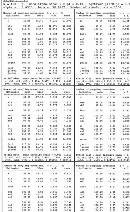
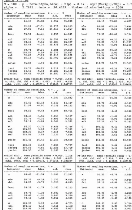
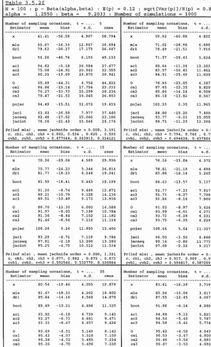
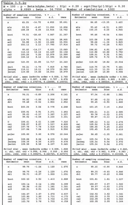
Conditional on the event C = {Z > X ,}, the mean, standard deviation and root
mean square error of each estimator are presented in ta
b
les l.la,
b,c, 1.2a,b,c, 1.3a,b,c
and 1.4a,b,c. These tab
les summarise the performance of the estimators for each
com
bination from the fo
llowing factorial design :
N
10
25
10
0.05
0
5
10
5 0 ^ t = i
5
X p =
0
.
10
x R = ^ ^ .
100
20
50
100
Note however that, for each value of population size N, onl
y v
alues of R up to and
including N are considered; this is done for o
bvious practica
l reasons.
The notation used within each ta
b
le is as follows :
Statistics
mean or expectation,
standai'd deviation,
root mean square error.
1 ~ Pro
b(C) = Prob(c) = Prob(Z = X j, which is the
probabi
lit
y o
f the maximum likelihood estimator
producing an infinite estimate.
exp.
s.d.
rmse
P(inf mle)
Estimators
X
I
=
P
=
CUE =
MLE =
p ’
X j,
the number of distinct individua
ls seen from the
target population.
the Peterson-t
yp
e estimator of section 1.7.
the conditionall
y unb
iased estimator of
section 1.8.
N ,
the maximum likelihood estimator of section
order to obtain the conditiona
l distri
bution of the Peterson-t
yp
e estimator Np given C
we need to derive the conditional distri
bution of X, and X^ given C. This ma
y b
e done
as follows :
C is defined as
being the event {Z> X,}.
Let C be the comp
lementai
y
event {Z = X ,}.
C occurs
<=>
X
2
= 0
and
each animal in target population is seen at
most once.
Now Pro
b(X
2
=
0
) = |(
l - p)‘J .
(1.13)
( This follows from the fact that Xg ~ Bin^R, 1 - (l - p)'
J.
)
Let Yj = the num
ber of sightings of anima
l i, it follows that
Y- ~ Bin(t,p).
It ma
y
then
be observed that
Prob( each anima
l in target population is seen at most once )
N
=
<
1
)
i=l
= [ ( l - p + tp)(l-p)'"']'*.
(1.14)
Use of (1.13) and (1.14) implies that
Pro
b(C) =
l-P ro
b (c )
= 1 - [(1 - p)' ]" [(1 - p + tp)(
l - p)'"' ]".
Now
_ Pro
b(Xj =Xi,X
2
=X
2
)Prob(Z>Xi|Xi = X;,X
2
= X
2
)
Prob(Z > X, )
Prob(Xi =Xj )Prob(X
2
=X
2
)Prob(Z>X] |X, =Xj ,X
2
=X
2
)
”
Prob(Z>X,)
‘
It is c
lear that Pro
b(Z > X,|Xj = XpX
2
= X
2
) = 1 if Xj > 0.
When X
2
= 0 it ma
y b
e o
bserved that Z|Xi,X
2
= ZjX^ . It is known that the
distribution of Zi|X, ma
y b
e characterised as
being the sum of Xj zero truncated
Binomia
l random varia
b
les, the distri
bution of which is derived in appendix 3.
Exp
licitl
y
the pro
babi
lit
y
function of ZjX^ is given
b
y
P
ro
b(Z, = z,|X, =
X , )=
5(x„z, ;t,0 ),
[ l - ( l - p ) J
Pro
b(Z > Xi|X, = XpX
2
= X
2
) = Prob(Zj > xJXj = x j
= 1 - Prob(Zj = xJXj = Xj)
_ ,
t - p - ( i - p r - ^ '
[
i-(i-p)T
’Using the notation P(C) = Prob(Z > XjXj = Xj,X
2
= X
2
) then a
llows one to write :
-5(xi,Xi;t,0)
using L3a.
Pro
b(Xi=XpX2=X2|Z>Xi)=—
P(C)
_ fO,
l,2,...,N for R > 0
1.2....,N
for
R = 0 ’
1.2....,R
for R > 0 , Xi =0
0,1,2,...,R for R > 0 , x^>0,
0 for
R = 0
X