Pruning Rules for Optimal Runway Sequencing
Geert De Maere, Jason A.D. Atkin
ASAP research group, School of Computer Science, University of Nottingham, NG81BB Nottingham, UK {gdm,jaa}@cs.nott.ac.uk
Edmund K. Burke
Queen Mary University of London, Office of the Principal, Queens Building, Mile End Road, London, E14NS, UK [email protected]
This paper investigates runway sequencing for real world scenarios at one of the world’s busiest airports,
London Heathrow. Several pruning principles are introduced that enable significant reductions of the
prob-lem’s average complexity, without compromising the optimality of the resulting sequences, nor compromising
the modelling of important real world constraints and objectives. The pruning principles are generic and
can be applied in a variety of heuristic, meta-heuristic or exact algorithms. They could also be applied
to different runway configurations, as well as to different variants of the machine scheduling problem with
sequence dependent setup times, the generic variant of the runway sequencing problem in this paper. They
have been integrated into a dynamic program for runway sequencing, which has been shown to be able to
generate optimal sequences for large scale problems at an extremely low computational cost, whilst
consid-ering complex non-linear and non-convex objective functions that offer significant flexibility to model real
world preferences and real world constraints. The results shown here counter the proliferation of papers that
claim that runway sequencing problems are too complex to solve exactly and therefore attempt to solve
them heuristically.
Key words: Dynamic programming, Runway Sequencing, Machine Scheduling, Sequence dependent setup times
History:
1.
Introduction
The recent and predicted future growth in air transport (Eurocontrol 2013) has already increased the pressure on airport resources around the world, and will continue to do so. This is especially true in the case of runways at highly congested airports that already operate at or close to their maximum capacity. Runway capacity often limits the overall airport capacity, thus the efficient use of this scarce resource is particularly important; failure to do so can significantly increase delays, aircraft emissions and costs for airlines. Adding extra runway capacity (i.e. new runways) is expensive, requires long term planning and may not be possible at many airports due to space restrictions. However, improved use of existing runways may be achieved by intelligently schedul-ing runway operations by re-sequencschedul-ing aircraft. This is complex to achieve and requires highly sophisticated algorithmic approaches to be embedded within complex decision support systems to assist runway operators. Such algorithms must be fast enough to allow their use in highly dynamic environments.
Since different separations have to be maintained between aircraft of different types (see Section 2), the order in which aircraft use the runway will affect the overall runway throughput and the delays for each aircraft. The problem of determining this order is called the runway sequencing problem. It aims at finding a feasible sequence that meets all constraints and has a satisfac-tory or optimal value for some given objective function(s). Many constraints apply to the runway sequencing problem, such as ensuring that safe separations are always maintained between aircraft, ensuring that aircraft are not scheduled to use the runway before they can get there, and meeting any landing/take-off deadlines which may apply to aircraft. There will usually also be a number of conflicting objectives (Atkin et al. 2010, Atkin 2013, Bennell et al. 2011), such as to maximise the runway utilisation, to reduce the average delay per aircraft, and to ensure some level of fairness between the delays for different aircraft. Full details of the problem are provided in Section 2.
therefore has more, and more complex, constraints than the arrival sequencing problem, for which only the weight classes of the aircraft influence the separations. I.e. separation rules for departures usually do not have such simple structures in them that can be exploited for simplifying the problem. For this reason, the focus of this paper is upon the departure sequencing problems in complex real world environments. Experiments have shown that the approach is also applicable for arrival problems, and that these are actually much easier for it to solve, as will be observed in Section 4.2.
A number of exact approaches for the runway sequencing problem have been introduced previ-ously, and are discussed in more detail below. Heuristic approaches were introduced by, for example, Atkin et al. (2007) and Bianco et al. (1999). We refer the reader to Bennell et al. (2011) for an extensive survey of previous approaches.
Psaraftis (1980) utilised the characteristics of the problem to design an approach which grouped identical aircraft into a number of queues, one per aircraft type, and exploits the fact that a known precedence order exists within the queues in terms of total processing cost. The proposed dynamic program to solve the problem of interleaving queues is polynomial as a function of the number of aircraft nand exponential as a function of the number of aircraft types N (O(N2(n+ 1)N). Such an approach is practical for arrival sequencing, where there may be up to six or seven
queues (N), but is impractical for take-off sequencing or mixed mode sequencing (simultaneous arrivals and departures) since many more queues are required in these cases (due to the more complex separations, up to 33 queues for the problem instances considered in this paper). Psaraftis further enhanced his approach by utilising constrained position shifts, introduced by Dear (1976). Constrained position shifts restrict an aircraft’s maximum positional shift relative to its position in the initial sequence, usually in first come first served order. This not only reduces the number of aircraft which have to be considered for each position in the sequence, but also enforces equity by preventing individual aircraft from being advanced or delayed disproportionally.
Constrained position shifts were also applied in the dynamic program introduced by Balakrishnan and Chandran (2010). Their approach has a complexity that is polynomial as a function of the number of aircraft n and exponential as a function of the constrained position shift k (O(n(2k+ 1)(2k+2))). The authors also presented an extension of the approach to allow the optimisation of more complex objective functions, albeit at an increased computational complexity.
sequences, thereby challenging the tractability and practicality of approaches based on them. We refer the reader to Atkin et al. (2007) and Atkin et al. (2010) for a more detailed discussion of why large positional delays are sometimes beneficial rather than harmful.
If the objectives can be (at least piecewise) linearised, the problem can potentially be solved using a MILP (Mixed Integer Linear Programming) solver such as CPLEX. Beasley et al. (2000) and Ernst et al. (1999) applied such an approach for the arrival scheduling problem with hard landing time windows. Beasley et al. (2000) introduced a mixed integer 0-1 formulation for the static, mixed or segregated, single or multiple runway sequencing problem. The approach exploits the presence of disjoint intervals due to relatively narrow hard time windows for arrivals (caused by speed and fuel limitations), applying a similar sort of simplification as for constrained position shifts, but utilising landing time rather than landing position. The approach allows the modelling of precedence constraints, complex separation matrices and complex piecewise linear and non-linear cost functions through time discretization and linearisation. Additional constraints are added to strengthen the formulation and improve its tractability.
In summary, a number of approaches have been developed in the past to simplify the runway sequencing problem, utilising the characteristics of the problem to do so. However, the assumptions which underlie these approaches fail to hold for departure or mixed mode sequencing, where large position shifts can be necessary for high quality results and time-windows are usually large (or open-ended) and may overlap with many other windows (preventing them from being used to simplify the problem). In addition, real world departure sequencing problem instances often require the consideration of complex objective functions that model trade-offs between multiple individual real world preferences (including delay, equity of delay, and time window compliance), further increasing the challenging nature of this problem.
Pruning rules have received considerable attention in the literature on machine scheduling and help to improve tractability (Allahverdi et al. 1999, 2008). However, the majority of these approaches do not consider sequence dependent setup times, nor complex non-convex, non-linear, or discontinuous objective functions such as the one considered here. Earlier work on dominance rules that did consider sequence dependent setup times includes Ragatz (1993) and Bianco et al. (1999). Ragatz (1993) introduces a branch and bound algorithm to optimise total tardiness and prunes the search tree when local improvements can be achieved through a pairwise interchange of jobs without increasing the future cost. Similar approaches that exploit local improvement strate-gies were introduced by Luo and C. Chu (2007) for the maximum tardiness problem, Sourd (2005) for the earliness-tardiness problem, and by Luo et al. (2005) and Luo and Chu (2006). The branch and bound approach presented by Sewell et al. (2012) maintains a set of non-dominated solutions during the exploration of the search tree, and uses the set to establish dominance relationships for the current branch.
In contrast to approaches which reduce the search space by limiting the movement of aircraft within the sequence, the pruning of the search space introduced here exploits (in most cases) characteristics of the objective function to infer that the current sequence, or any future sequences based on it (by appending aircraft to it), is sub-optimal. Whilst the characteristics are investigated in the context of the objective function considered here, it can be easily shown that many of them transfer to other objective functions that are commonly considered in the literature. The advantage of exploiting characteristics of the objective function in the pruning rules is that partial sub-sequences which show known poor characteristics can be pruned much earlier, even before the dominating partial sequences have been generated. In addition, our pruning rules often have a much lower complexity when compared to some of the the pruning rules based on local improvements used in the approaches for machine scheduling listed above, and they are therefore usually more effective from a computational point of view.
machine scheduling carried out by Panwalkar and Iskander (1977) reports that 70% of schedulers state that setup times are sequence dependent in about 25% of the cases, and that the exact setup times depend on the degree of similarity between jobs, and hence are well structured. Given that the runway sequencing problem considered here is cast as a single machine scheduling problem with sequence dependent setup times, and considering the observation that many real world instances of such problems are well structured, our approach is expected to be applicable to a wide variety of similar problems, and could therefore have a significant impact on a large number of real world applications.
2.
Problem description and model
Given a set of aircraftS, with (asymmetric) minimum separationsδij between any ordered pair of
aircraftiandj (whereiprecedesj), the runway sequencing problem consists of finding a sequence of landings and take-offs, s, such that an optimal (or acceptable, for heuristic methods) value is achieved for some given objective function(s), subject to the satisfaction of all hard constraints.
2.1. Constraints
A feasible sequence must meet minimum runway separations,hard time windows (if applicable), and earliest take-off times. Any sequence that violates these constraints is not feasible in practice, and can be eliminated from the solution space.
2.1.1. Separation Constraints For the departure instances considered here, the minimum runway separations are determined by the aircraft’s weight classes, speed groups, and their standard instrument departure routes (SIDs). An aircraft’s weight class determines the severity of the wake turbulence it causes, the time that is required for this to dissipate, and its senstivity to wake turbulence caused by other aircraft. Larger aircraft generate, in general, more turbulence, to which smaller aircraft are more sensitive. Consequently, a larger weight class separation is required when a large aircraft is followed by a small aircraft, than when a small aircraft is followed by a large aircraft (i.e. the separations are asymmetric). In a similar fashion, larger speed group separations may be required when a slower aircraft is followed by a faster aircraft on the same route. This is necessary to prevent the following aircraft from catching up before their routes diverge. Minimum departure route separations are influenced by the climb and the relative bearing of the route, as well as congestion in downstream airspace sectors. The latter may require an increased separation upon take-off, to space out traffic and prevent the overloading of en-route sectors and controllers. The minimum separation that must be maintained at the runway between the take-off time of two (departing) aircraft is equal to the maximum of their weight, speed, and SID separation. This results in a well structured separation matrix. For instance, the required separation for a fast and small aircraft is usually no less than the separation for a slow and large aircraft if they follow the same aircraft on the same route. However, the resulting separation matrix does not necessarily obey the triangle inequality. I.e., given three aircraft i,j, and k using the runway in the order i, thenj, thenk with the respective required separations between them denoted byδij,δjk, and δik,
thenδij+δjk≥δikdoes not necessarily hold. The take-off time of one aircraft (e.g.k) can therefore
be influenced by multiple-preceding aircraft (e.g.,i and j).
2.1.2. Time Windows Let aircraftibe subject to a hard time window (that must be adhered to) that is defined by its start time eti and end time lti, then its take-off time, ti, must be within
can be considered to be subject to a very large time window with start time eti equal to −M and
end time lti equal to +M, with M denoting a very large constant (large enough to not interact
with the aircraft times).
In addition to a hard time window, an aircraft which is taking off can be subject to a Calculated Take-Off Time (CTOT) or slot. A CTOT is a 15-minute time window during which the aircraft should take-off. Let the start and end time of the CTOT window for aircraft i be denoted byeci
and lci respectively. An aircraft cannot take-off before eci and may have to be delayed to meet
the start of its window. It preferably takes-off before its end, lci. Although their use is strongly
discouraged and penalised, a limited number of 5 minute (300 seconds) CTOT extensions have been available and could be used for aircraft that would otherwise narrowly miss their CTOT. The start time of a CTOT window is therefore modelled as a hard constraint and the end time is modelled as a heavily penalised soft constraint or objective.
2.1.3. Earliest Take-Off Time Assuming that the earliest time an aircraft i can join the queue of aircraft waiting at the runway for take-off is bi (which we name the “base time”) and
that the minimum time to reach the start of the queue and line up with the runway is ci seconds,
the earliest time aircraftican be sequenced, irrespective of any other aircraft, is called the release timeri and can be calculated as the maximum ofbi+ci and the start times of any hard or CTOT
windows (eti and eci). This is shown in Equation 1.
ri= max(bi+ci, eti, eci) (1)
Assuming that each aircraft will be sequenced as early as possible (which is a valid assumption at busy airports), the time ti for aircraft i is equal to the maximum of ri and tx+δxi for all x∈si,
where x denotes an aircraft in the partial sequencesi of aircraft which take-off beforei and tx its
take-off time. This is defined by Equation 2, in which ri can be substituted by Equation 1.
ti= max(ri,max x∈si
tx+δxi) (2)
2.2. Objectives
The objective function, F(s), considered in our approach is defined by Equation 3 and models runway utilisation (quantified by the take-off time of the last aircraft in the partial or final sequence that contains all aircraft in the set, i.e. the makespan), total (non-linear) delay, and CTOT compli-ance. The runway utilisation is determined by the take-off time of the last aircraft in the sequence sand is equal to max
x∈s tx. Apart from its meaning as an objective (since it reflects runway
The objective function for delay and CTOT compliance is defined by the second component in Equation 3.
F(s) = (max
i∈s ti, P
i∈s
(W1(ti−bi)α+W2C(ti, lci))) (3)
C(ti, lci) =
0 if ti≤lci
ω1(ti−lci) +ω2 if lci< ti≤lci+ 300
ω3(ti−lci) +ω4 if ti>(lci+ 300)
(4)
The delay cost for an aircraft iis calculated as a function of the difference between its base time bi and its take-off time ti, and measured as W1(ti−bi)α, where W1 and α are constants (α≥1) which can be set to appropriate values to model controller preferences (Atkin et al. 2010). Larger values of α penalise larger delays more severely and encourage a more equitable distribution of delay.
The cost for CTOT violations in Equation 3 is given by W2C(ti, lci), in which W2 denotes a constant. C(ti, lci) is a non-convex discontinuous piecewise linear function that is defined by
Equation 4, in which ω1, ω2, ω3, ω4 represent constants. The different segments of C(ti, lci) reflect
the different costs associated with an aircraft taking off within its CTOT window (eci≤ti≤lci),
narrowly missing its departure window but leaving no more than 300 seconds late (lci < ti ≤
lci+ 300), or missing its CTOT window completely (lci+ 300< ti). Given the increasing degree
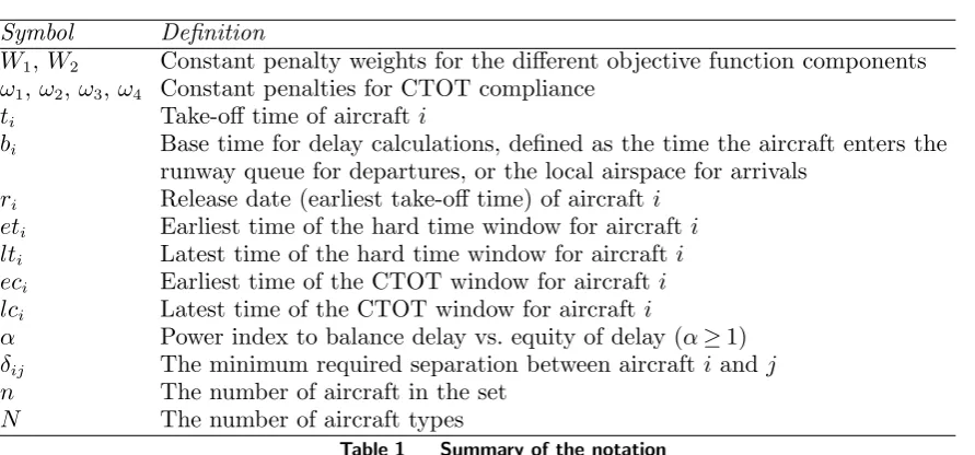
of severity of missing a CTOT and hitting an extension, and missing CTOT and its extension completely, it is usual thatω1<< ω3 and ω2<< ω4. This results in a jump in cost in the objective function that recognises that small time window extensions are sometimes possible for departures but should be avoided, whereas missing an extension is extremely bad. We note that the trade-off between delay cost and slot compliance in Equation 3 can be influenced by setting their weight factors (W1 and W2) appropriately. A summary of the notation is provided in Table 1.
Symbol Definition
W1,W2 Constant penalty weights for the different objective function components ω1,ω2,ω3,ω4 Constant penalties for CTOT compliance
ti Take-off time of aircrafti
bi Base time for delay calculations, defined as the time the aircraft enters the
runway queue for departures, or the local airspace for arrivals ri Release date (earliest take-off time) of aircrafti
eti Earliest time of the hard time window for aircrafti
lti Latest time of the hard time window for aircraft i
eci Earliest time of the CTOT window for aircrafti
lci Latest time of the CTOT window for aircraft i
α Power index to balance delay vs. equity of delay (α≥1) δij The minimum required separation between aircraft iand j
n The number of aircraft in the set
[image:10.595.76.522.69.277.2]N The number of aircraft types
3.
Pruning rules and solution method
This section introduces six pruning principles that can significantly reduce the solution time for real world runway sequencing problems, without losing optimality. They also apply to other machine scheduling problems with sequence dependent setup times that have objectives and structures similar to the runway sequencing problem. The pruning rules are explained in this section along with proofs that solution optimality is not lost by using them. A discussion of the applicability and performance of each rule to runway sequencing problems and other setups in which they hold is also given. Finally, the section ends with a description of the dynamic programming method which was developed to solve the runway sequencing problems and is used in Section 4.
Our pruning principles are:
1. A multi-objective extension of the ability to infer a complete order within sets of separation identical aircraft (Psaraftis 1980) for the non-additive objective function considered here
2. The ability to infer conditional orders between sets of separation identical aircraft 3. The ability to infer conditional orders between sets of non-separation identical aircraft 4. The use ofinsertion dominance which prunes sequences with intrinsically bad characteristics 5. The use of dominance combined with lower bounding
6. The identification of more generic dominance rules between partial sequences (i.e. to which other aircraft still have to be added to the end) that cover non-identical sets of aircraft
The first principle results in the generation of a number of distinct sets of aircraft. The remaining principles result in a tight coupling between those aircraft sets and enable new dominance relations to be inferred between partial sequences. All principles can be applied to prune partial sequences and are therefore particularly useful in algorithms that generate sequences by adding one aircraft at a time, such as the dynamic program used here (described in Section 3.7) or, e.g., branch and bound algorithms. However, they are also useful in other algorithms that are working on complete sequences (containing the entire set of aircraft), e.g. to verify whether a particular change to the sequence will compromise its optimality.
3.1. Definitions
For the following proofs, letiandjdenote two aircraft that areseparation identical, i.e. the mutual separations for aircraft i and j with respect to all other aircraft x in the set S (which includesi and j) are the same (δix=δjx, δxi=δxj ∀x∈S). Let k denote an aircraft that is not separation
identical toi, i.e.∃x∈S:δix6=δkx orδxi6=δxk. Aircraftkis said to be “more difficult” to sequence
than aircraft i with respect to a set of aircraft S if the mutual separations between k and any aircraftx∈S are no less than the respective separations between iand x, and strictly greater for at least one aircraft x∈S (i.e. δkx≥δix, δxk≥δxi ∀x∈S and ∃x∈S:δkx> δix orδxk> δxi).
Let the base times for i, j, and k be denoted by bi, bj, bk, respectively, the start times of the
hard and CTOT windows be denoted by eti, etj,etk and eci, ecj, eck, respectively, and the ends
of hard and CTOT windows be denoted by lti,ltj,ltk and lci,lcj,lck, respectively. Finally, let tx
denote the take-off time of aircraftx in sequencesand t0x denote the take-off time of aircraftxin
sequences0.
3.2. Complete orders within sets of separation identical aircraft
A complete order exists between aircraft i and j if the objective value(s) and feasibility of any arbitrary sequence sincludingiand j cannot, under any circumstances, be improved by reversing the order of i and j ins. If such complete orders exist, the sequencing problem can be simplified to one of interleaving ordered sets of aircraft, always sequencing the first available aircraft from the respective sets. The existence of such complete orders between separation identical aircraft was shown by Psaraftis (1980) for the optimisation of processing cost, enabling a reduction in the complexity of the problem from factorial as a function of the number of aircraft n (i.e. n!) to exponential as a function of the number of aircraft types N, and equal toO(N2(n+ 1)N).
In a multi-objective context, a complete order may be inferred upon a set of aircraft if the complete orders for each of the individual constraints and objectives are consistent within the set. The formal proofs below show that this is the case for the makespan and delay objectives, even with hard time window constraints if the base times (bi), release dates (ri), and the end times of
hard time windows (lti) of the individual aircraft are in order. However, this is not the case for the
cost incurred by CTOT windows.
3.2.1. Initial observations We first present some initial observations which can be used to simplify later proofs.
Lemma 1. Given two sub-sequences sand s0 with identical aircraft in the same order, differing
only in the take-off times (e.g. due to different aircraft preceedingsands0), iftx≤t0xfor all aircraft
x in s and s0, the delay (or CTOT) cost for each individual aircraft in swill be no worse than its
delay (or CTOT) cost in s0, and the total delay (or CTOT) cost summed over all aircraft in swill
Proof: Delay (or CTOT) costs monotonically increase with time, hence the pairwise cost rela-tionship holds between corresponding aircraft. The relarela-tionship for the total cost summed over all aircraft insthen follows.
Lemma 2. Given two sub-sequences sand s0 with identical aircraft in the same order, differing
only in the take-off times, iftx≤t0x for all aircraftx in sand s0, the violation of an aircraft’s hard
time window in swill be no worse than its violation in s0, and hence if sequence sis infeasible, so
will be sequence s0.
Proof: Since the aircraft order insands0is identical, and sincexcannot be sequenced beforeetx
and can always be delayed to meetetx,tx≥etxis trivial. Sincetx≤t0x, ift0x≤ltx, thentx≤t0x≤ltx,
hence any aircraft xins cannot violate the time window ins(i.e. tx> ltx) if x does not ins0 (i.e.
t0x> ltx).
Lemma 3. Given two aircraft setsAandA∪x, the delay (or CTOT) cost for a sequencesbased
onAis no less than the delay (or CTOT) cost for a sequences0 ofA∪xwith identical aircraft order
for the aircraft in A and with x inserted at any arbitrary position, both with or without including
the cost for x (without considering the cost of the aircraft remaining to be added).
Proof: Inserting an additional aircraft in any sequence cannot decrease the times for subsequent aircraft. The delay (or CTOT) cost is monotonically increasing and the delay (or CTOT) cost for x is non-negative (Equation 3).
Lemma 4. Let s and s0 denote two sequences based on the sets A and A∪x, respectively, for
which the order of the aircraft in A is the same in s and s0, and with x inserted at any arbitrary
position in s0 (i.e. not appended). The violation of hard time windows for s is no less than fors0,
both with or without considering the violation forx, and without considering the cost of the aircraft
remaining to be added.
Proof: Inserting an additional aircraft in any sequence cannot decrease the times for subsequent aircraft. It then follows that violations of hard time windows cannot decrease (Lemma 2).
3.2.2. Makespan
Theorem 1. An objective to minimise makespan can be considered to induce a complete order
Proof: Let s denote a partial sequence containing iand j (in that order), and lets0 denote a
partial sequence with identical order except that iand j are reversed. Let the times allocated to i and j be denoted by ti and tj for s, and by t0i and t
0
j for s
0. We will prove that if r
i≤rj, then
any sequence with prefixswill be no worse than the equivalent sequence with prefix s0, and hence a complete order may be inferred betweeniand j for makespan. The proof has four components. Firstly we show that ti≤t0j. Secondly, we show through induction that the corresponding times
for the aircraft betweeniandj ins(jand iins0) are no later insthans0. Thirdly, we show that tj≤t0i. Fourthly, we show that the inductive proof in the second part therefore also holds for any
further aircraft which could be added to the end ofsand s0, completing the proof.
Part 1: Let si and s0j denote the identical partial sequences of aircraft which are sequenced
before i in s and before j in s0. Given the definitions of s and s0, s
i=s0j. From Equation 2 we
know ti=max(ri, tx+δxi ∀x∈si) andtj0 =max(rj, tx+δxj ∀x∈si). Sinceiand j are separation
identical andri≤rj, then ti≤t0j.
Part 2: Let y denote any aircraft betweeniand j in s(between j and iins0) such that t
y and
t0
y denote the times ofy ins and s0, respectively. Let sy denote the sequence of aircraft which are
before y in s and let s0
y denote the sequence of aircraft which are before y in s0. From Equation
2 we know ty=max(ry, tx+δxy ∀x∈sy) and t0y=max(ry, t0x+δxy ∀x∈s0y). By consideration of
corresponding terms between the two equations,ty≤t0y iftx≤tx0 for allx prior toy.tx=t0x for all
x∈si, since the aircraft are identical, andti≤t0j (from part 1). Thus, by induction ty≤t0y for all
y between iand j ins.
Part 3: Letsjdenote the partial sequence of aircraft beforejinsand lets0idenote the sequence of
aircraft beforeiins0. From Equation 2,t
j=max(rj, tx+δxj∀x∈sj) andt0i=max(ri, t0x+δxi∀x∈
s0
i). From part 2, we know thatt
0
x0≥tx for all xand x0 at corresponding positions in sj. Since j is
sequenced before iins0,t0
i≥rj, and thust0i≥tj.
Part 4: The inductive proof from part 2 therefore also applies to tj and t0i, and, thus, to all
subsequent aircraft, including the ones which will be added to the end of the sequence.
Lemma 5. Given the definitions of s, s0, ti, tj, t0i, t0j in the proof of Theorem 1, ti≤t0j≤tj≤t0i
holds.
Proof: The sequence of aircraft prior to j in s0 is a sub-sequence of the sequence of aircraft
prior toj ins, thus t0
j≤tj. From Theorem 1, ti≤t0j and tj≤t0i.
Proof: This is a direct consequence of Theorem 1.
Lemma 7. If an aircraft x is appended to both of the sequences s and s0 defined in Theorem 1
with times tx and t0x respectively, then tx≤t0x.
Proof: The inductive proof of Part 4 also applies to aircraft x, and to any subsequent aircraft.
3.2.3. Delay
Theorem 2. An objective to minimise the cost for delay in Equation 3 can be considered to
induce a complete order upon two separation identical aircraft i and j where bi≤bj and ri≤rj.
Proof: Assume the same definitions fors,s0,t
i,tj,t0i,tj0 as in Theorem 1.tx≤t0x0 for all aircraftx
andx0 in corresponding positions insands0respectively (Lemma 6) and delay costs monotonically
increase (Lemma 1). An objective to minimise delay can therefore induce a complete order uponi and j if Inequality 5 holds:
W1(ti−bi)α+W1(tj−bj)α≤W1(t0j−bj)α+W1(t0i−bi)α (5)
Since the conditions for Lemma 5 hold, we know ti≤t0j≤tj≤t0i, so we can define x1, x2, x3≥0 such thatt0
j=ti+x1,tj=t0j+x2=ti+x1+x2,t0i=tj+x3=ti+x1+x2+x3. Inequality 6 is then equivalent to Inequality 5.
(ti−bi) α
+ (ti+x1+x2−bj)
α≤
(ti+x1−bj) α
+ (ti+x1+x2+x3−bi) α
(6)
Letx2= 0, then Inequality 6 becomes Inequality 7 or 8, which holds for allx1, x3≥0.
(ti−bi)α+ (ti+x1−bj)α ≤(ti+x1−bj)α+ (ti+x1+x3−bi)α (7)
(ti−bi)α ≤(ti+x1+x3−bi)α (8)
Thus, Inequality 6 holds for x2= 0. As x2 is increased (ti+x1+x2+x3−bi)α will increase
faster than (ti+x1+x2−bj)α, sincebi≤bj and x3≥0. Inequalities 5 and 6 therefore hold for all x1, x2, x3≥0, thus the cost of s can be no greater than the cost of s0, so there is never a benefit from sequencing j beforei.
3.2.4. Time windows
Theorem 3. Hard time windows can be considered to induce a complete order upon two
sepa-ration identical aircrafti and j whereri≤rj and lti≤ltj
Proof: Assume the same definitions of s,s0,t
i,tj,t0i,t
0
j as in Theorem 1. Since an aircraft can
always be delayed to meet the start of its window,etx≤tx is trivial. Sincetx≤t0x0 for all aircraftx
and x0 at corresponding positions insand s0 (Lemma 6), the time window violation of all aircraft other thaniandj is no worse insthan ins0 (Lemma 2). Ifimisses its hard time window ins(i.e.
ti> lti), irrespective ofj,iwill also miss its time window ins0, sincet0i≥ti, thust0i> lti. Ifjmisses
its time window in s(i.e.tj> ltj), then iwill miss its time window ins0, sincet0i≥tj and lti≤ltj.
Since tx≤t0x (Lemma 7) for any arbitrary aircraft x added to both s and s0, the time window
violation forx is no worse in the case ofs. Hence, a complete order can be inferred betweeniand j for time window violations.
Lemma 8. A complete order can be inferred within a set of separation identical aircraft with
respect to makespan, delay, and hard time window compliance if the base times (bx), release dates
(rx), and the end times of hard time windows (ltx) are in the same order for all aircraft x in the
set.
Proof: The necessary conditions for Theorem 1 (the release dates are in order), Theorem 2 (the base times and release dates are in order), and Theorem 3 (the release dates and end times are in order) are satisfied for all ordered pairs of aircraft in the set, hence a complete order can be inferred.
In contrast to Lemma 8, complete orders cannot be inferred within separation identical sets when CTOT windows are considered due to the piecewise linear, discontinuous and non-convex objective function that models their cost. I.e., the better order for two separation identical aircraft i and j (bi≤bj,ri≤rj, lci≤lcj) depends upon the times ti and tj. For example, let us assume
that j is restricted by a CTOT window but i is not. Let s denote a partial sequence in which i is sequenced at time ti≥rj (i.e. after j becomes available for sequencing), and j is sequenced at
time tj ≥lcj (i.e., j misses its time window). Since ti≥rj, and i and j are separation identical,
the aircraft could be swapped with no modification of times toi,j, or other aircraft. Even though the swap may potentially increase the delay cost (sincebi≤bj,ri≤rj) the reduction in the CTOT
sequencing j before i, since this would not reduce j’s CTOT violation cost, so the total cost for i and j (see §3.2.3) would not improve and could even increase.
If bothiandjare subject to a CTOT, then the lower cost order will depend upon the relationship between ti, tj,eci,ecj,lci, andlcj. Given the CTOTs for iand j and the possible times at which
iand j can be scheduled, say t1 and t2, witht1< t2, if both aircraft can meet their time windows with i scheduled before j (i.e., ti=t1≤lci and tj=t2≤lcj), then i should precede j for reasons
of delay. However, iflci≤t1< lcj≤t2 then swapping the aircraft so that tj=t1 and ti=t2 would mean that only imisses its time window. This could result in a lower total CTOT violation cost which could more than offset the increased delay cost.
Performance: An efficient algorithm would implement complete orders by generating and order-ing the separation identical sets in a pre-processorder-ing step, i.e. before the actual sequencorder-ing is done. This can be done through pairwise comparison of aircraft and their separations with the aircraft in the setS. The solution method can then interleave the ordered sets by selecting the first avail-able aircraft in each of the sets and avoid consideration of later aircraft. If the solution method is exact, optimality of the resulting sequences will not be compromised since a complete order exists within the sets. It was shown by Psaraftis (1980) that interleaving ordered sets of aircraft reduces the worst case complexity from n! to O(N2(n+ 1)N), with N denoting the number of sets and n
denoting the number of aircraft. I.e., complete orders reduce the computational complexity of the algorithm and require no additional computation during its execution.
The efficacy of using complete orders is highly influenced by the complexity and structure of the separation matrix, and the aircraft mix that operates at the airport in practice. In practice, the separation matrices for runway sequencing problems have a structure which enables complete orders to be exploited well. However, in extreme cases, e.g., where all aircraft are subject to a CTOT, when the aircraft mix is highly diverse, or when no separation identical aircraft are present, no complete orders can be inferred. Even in this case, however, the pruning rules introduced below can help to improve tractability.
3.3. Conditional orders
Theorem 4. A conditional order can be inferred between two separation identical aircraftiand
j (ri≤rj,lti≤ltj), such thatishould precedej, whenti,tj, t0i,t0j are such that Inequality 9 holds.
W1(ti−bi)α+W2C(ti, lci) +W1(tj−bj)α+W2C(tj, lcj)≤
W1(t0i−bi)α+W2C(t0i, lci) +W1(t0j−bj)α+W2C(t0j, lcj) (9)
Proof: Let us assume the definitions of s, s0, ti, tj, t0i, t
0
j in Theorem 1. Since ri≤rj and
lti≤ltj, a complete order can be inferred between i and j with respect to makespan and hard
time window violations. Hence,tx≤t0xfor all aircraft other thaniandjat corresponding positions
in s and s0 (Lemma 6), or at corresponding positions in sequences obtained by adding a
sub-sequence containing the same aircraft in the same order to s and s0 (Lemma 7). It then follows that sequencing j before i could not decrease the makespan, the delay cost, the CTOT violation cost, and the violation of hard time windows for any of these aircraft (Lemmas 1 and 2). Hence, an order can be inferred between i and j such that i should precede j if Inequality 9 holds, and thus the cost for sequencingibefore j is lower than the cost of sequencingj beforei.
Theorem 5. If tj and t0i are not yet known (e.g. when incrementally building up the sequence),
a conditional order can still be inferred betweeniand j if, in addition to the conditions outlined in
Theorem 4, bi≤bj, lci≤lcj and Inequality 10 hold.
W1(ti−bi)α+W2C(ti, lci)−W1(t0j−bj)α−W2C(t0j, lcj)≤
W1(t0i−bi) α
+W2C(t0i, lci)−W1(t0i−bj)
α−
W2C(t0i, lcj) (10)
Proof: If ri≤rj, lti≤ltj, and bi≤bj, a complete order can be inferred between i and j for
makespan, delay, and hard time window violations. Since delay costs are monotonically increasing and tj≤t0i (Lemma 5), W1(t0i−bj)α≥W1(tj−bj)α, and thus W1(t0i−bi)α−W1(tj−bj)α≥W1(t0i−
bi)α−W1(t0i−bj)α. Since CTOT violation costs are monotonically increasing for ω1≤ω3 and ω2≤ω4 (Equation 4) andtj≤t0i (Lemma 5),C(t
0
i, lcj)≥C(tj, lcj), and thusC(t0i, lci)−C(tj, lcj)≥
C(t0
i, lci)−C(t0i, lcj). Meeting Inequality 10 is therefore sufficient for meeting Inequality 9, and a
conditional order can be inferred between iand j as soon as Inequality 10 is met.
Ifbi≤bj, the minimum value forW1(t0i−bi)α−W1(t0i−bj)αoccurs at minimalt0i. The minimum
value ofC(t0
i, lci)−C(t0i, lcj) occurs either at minimalt0i or around the discontinuities in Equation
4, and can therefore be calculated easily once an earliest time fort0
i is known, even before the exact
value for t0
is already in the partial sequence, and will increase as more aircraft are added, thereby further tightening Inequality 10.
A special case arises ifti≤lci(lci≤lcj), i.e. ifican meet its time window. In this case, Inequality
9 reduces to Inequality 11. A complete order exists for delay if ri ≤rj and bi≤bj, and thus
W1(ti−bi)α+W1(tj−bj)α≤W1(t0i−bi)α+W1(t0j−bj)α. From Equation 4, C(tj, lcj)≤C(t0i, lci)
forlci≤lcj,tj≤ti0 (Lemma 5), andC(t0j, lcj)≥0. Thus, Inequality 11 must hold and a conditional
order can be inferred between iand j ifri≤rj,bi≤bj,lti≤ltj,lci≤lcj and ti≤lci.
W1(ti−bi)α+W1(tj−bj)α+W2C(tj, lcj)≤
W1(t0i−bi)α+W2C(t0i, lci) +W1(t0j−bj)α+W2C(t0j, lcj) (11)
If ri≤rj, bi≤bj, and lti≤ltj and aircrafti and j are not subject to a CTOT window, their cost
is equal to 0, and Theorem 5 reduces to Lemma 8, in which case a complete order exists between i and j. Finally, if aircraft j does not have a CTOT window, Inequality 9 reduces to Inequality 12, which is always satisfied (since a complete order exists for delay, the CTOT window cost is monotonically increasing, and ti≤t0i, Lemma 5). I.e. a complete order exists between i and j in
this case.
W1(ti−bi)α+W2C(ti, lci) +W1(tj−bj)α≤
W1(t0i−bi)α+W2C(t0i, lci) +W1(t0j−bj)α (12)
3.3.2. Conditional orders between non-separation identical aircraft
Theorem 6. A conditional order can be inferred between two non-separation identical aircraft
i and k (i more difficult to sequence than k, ri≤rk, lti≤ltk) such that i should precede k if the
increased separations for i compared to k do not impose an additional delay for any subsequent
aircraft in the current partial sequence, or any aircraft remaining to be added to the current sequence
when ti, tk, t0i, t
0
k are such that Inequality 13 holds.
W1(ti−bi)α+W2C(ti, lci) +W1(tk−bk)α+W2C(tk, lck)≤
W1(t0
i−bi)α+W2C(t0i, lci) +W1(t0k−bk)α+W2C(t0k, lck) (13)
Proof: Let s denote a partial sequence containing i and k (in that order), and let s0 denote a partial sequence with identical order except that i and k are reversed. Let the set of aircraft remaining to be added to s and s0 be denoted by R. If no additional delays are incurred by the aircraft subsequent toiinsor by any aircraft inR(relative tos0), thent
x≤t0xfor all aircraft other
for these aircraft is thus no worse in s than in s0 (Theorem 1 and Lemmas 1 and 2). Since t
i≤t0i
(the sequence of aircraft before i in s is a subsequence of the aircraft before i in s0) and t
k≤t0i
(the increased separations for icompared to k do not impose additional delay), the observations for hard time windows in Theorem 3 remain valid. If Inequality 13 holds, the delay cost and the cost for CTOT violations for i and k is no worse in s than in s0 and a conditional order can be
inferred foriand k.
In a similar fashion as in §3.3.1, a conditional order can still be inferred between iand k even if the exact values oftk and t0i are not yet known. This is the case if the current increase in delay
and time window cost for scheduling irather than k is less than any future decrease in delay and time window cost when k and i are later added, as shown by Inequality 14 (a rearrangement of Inequality 13). We note that with respect to the cost for CTOT violations in Inequality 14, the observations from §3.3.1 remain valid.
W1(ti−bi)α+W2C(ti, lci)−W1(t0k−bk)α−W2C(t0k, lck)≤
W1(t0i−bi)α+W2C(t0i, lci)−W1(tk−bk)α−W2C(tk, lck) (14)
Performance: To infer conditional orders when incrementally building up a sequence, the con-ditions in Theorems 4, 5 and 6 must be validated between the newly added aircraft and both the aircraft preceding it in the sequence and the aircraft remaining to be added to the sequence. The complexity of validating conditional orders is therefore linear as a function of the number of aircraft inS, denoted by |S|, since any aircraft is either added to the sequence or remaining to be added. If complete orders are present in S, and hence a number of ordered separation identical sets has been defined, conditional orders have to be evaluated only for the first remaining aircraft in each of the N sets. In addition, they only have to be evaluated for aircraft that are either separation identical or are more difficult to sequence, and for which replacing them withjdoes not impose an additional delay on subsequent aircraft in the sequence (ifrj>> tx, aircraftj is likely to impose an
additional delay). The actual number of comparisons is therefore likely to be significantly fewer in practice. This makes the implementation of conditional orders very efficient from a computational point of view.
Extension: We note that conditional orders can be generalised to any arbitrary objective func-tion/constraints, or any number of aircraft, as long as their exact times in the sequence are known. Indeed, if a local improvement can be obtained without increasing the future cost, the partial sequence, or any sequence based on the unimproved order, is not optimal. This is also the case if the exact times oftj andt0i are not yet known, as long as it can be establised for the given objective
3.4. Insertion dominance
Theorem 7. If an aircraftx can be inserted into a partial sequence s(i.e. not appended)
with-out delaying any of the subsequent and remaining aircraft, the sequence s can be pruned without
compromising optimality.
Proof: Since x can be inserted into s without delaying any of the subsequent and remaining aircraft, the makespan, delay cost, cost for CTOT violations, and the violation of hard time windows for these other aircraft does not increase (Theorem 1 and Lemmas 1 and 2). Ifxis scheduled after s, its time can be no earlier than if it was scheduled withins, thus the makespan, delay cost, CTOT violation cost (which are monotonically increasing), and the violation of hard time windows for x can also be no less (Theorem 1 and Lemmas 1 and 2). Therefore, the sequence based on s and containing x can be no worse than the sequence based onsto whichx is appended later.
Performance: To evaluate insertion dominance, it is necessary to verify whether any of the remaining aircraftx∈Rcan be inserted intoswithout additional delay to the subsequent aircraft in s, or to the aircraft inR\x. In practice, since complete orders exist between the aircraft in the same separation identical set, it is sufficient to validate this dominance rule only for the first remaining aircraft in each of the sets, and only for the positions inswhere the maximum separation forxwith any arbitrary aircraft exceeds the makespan of s augmented with the minimum separation (i.e., it can still influence future take-off times). The complexity of evaluating insertion dominance is therefore linear as a function of the number of separation identical setsN, and linear as a function of the number of positions that need to be considered for insertion dominance as determined by the maximum separation (this is 2 for the problem instances considered here).
The efficacy of insertion dominance is influenced by three factors: the distribution of the release datesri; the accumulated delay; and the occurrence of violations of the triangle inequality in the
separation rules. If all release dates are equal, or it is a high delay situation, an aircraftx’s release date,rx, is less likely to delay its take-off time. I.e.,txis likely to be constrained by the separation
requirements only. Hence, the sequence may not contain idle time, so insertion dominance may not apply. However, if the separation rules violate the triangle inequality, i.e.δij≥δix+δxj (with
iprecedingj in s), it may be possible to insert x between iand j without causing any additional delay to other aircraft, and hence without increasing their cost. In this case, s can be pruned without compromising optimality. In practice, the efficacy of insertion dominance is determined by a complex interaction between these three key factors (release dates, delay, and separation rules). We therefore report empirical results on its efficacy in Section 4.
arbitrary objective function, provided that it can be easily verified that the cost for inserting an aircraft is less than the future cost for adding the aircraft later.
3.5. Dominance with lower bounding
The presence of sequence dependent separations that violate the triangle inequality (e.g. for depar-ture sequencing, mixed mode operations, or for multiple runway scenarios) means that the take-off time(s) and objective value(s) of future aircraft added to a given sequence scan be influenced by one or more preceding aircraft, typically the most recently sequenced ones. The set of aircraft in sthat influence the times of future aircraft is called the “separation influencing set” and consists of all aircraft x∈sfor which the separation constraints tx+δxy may be binding upon the take-off
time ty of any arbitrary aircraft y in the set of aircraftR remaining to be added tos. The set of
other aircraft in s, i.e. the ones that are not binding upon the take-off time of any aircraft y∈R is called the“non-separation influencing” set.
Since the separation influencing set can affect the take-off time of future aircraft, and hence their objective value(s), two sequences sand s0 are comparable only if their separation influencing
sets are the same if standard dominance rules are used. I.e. sequences is no worse than sequence s0 if F(s) ≤F(s0) and t
x≤t0x for all aircraft x in the separation identical sets. This problem
characteristic greatly increases the complexity of the problem by increasing the number of non-comparable sequences by a factor of m!, where m is the number of separation influencing aircraft. I.e., the requirement for separation identical sets to be the same can significantly reduce the efficacy of pruning rules.
The requirements on the separation identical sets ofsands0can be relaxed by integrating “look-ahead” or lower bounding strategies to consider the effects of aircraft in the separation influencing sets on the set of aircraft, R, that remain to be added to the partial sequence s. This enables the inference of dominance relations between otherwise incomparable sequences, and significantly increases the number of sequences that can be compared.
Theorem 8. Given partial sequences s and s0 that contain the same set of aircraft, and a set
of aircraft R which have not yet been added, any sequence based on s is no worse than a sequence
based on s0 if s is feasible, F(s)≤F(s0) and max
x∈s(tx+δxy, ry)≤maxx∈s0(t
0
x+δxy, ry) ∀y∈R
Proof: Let z be a sequence consisting of sub-sequence s followed by any (sub-)set of aircraft in R and let z0 be the sequence consisting of the sub-sequence s0 followed by the same (sub-)set
of aircraft fromR in the same order. Let ty and t0y denote the times for y∈R in sequencesz and
z0, respectively. Thenty≤t0y ∀y∈R, since max
x∈s(tx+δxy, ry)≤maxx∈s0(t
0
x+δxy, ry) ∀y∈R. It follows
Performance: To evaluate dominance with lower bounding, it is sufficient to identify all compa-rable sequences (i.e. sequences that contain the same set of aircraft but do not neccesarily have the same separation influencing set) and validate the conditions in Theorem 8. If the sequences are ordered and grouped by their aircraft set, the sets of comparable sequences can be located using binary search. I.e. the worst case complexity is given by O(log2 N), withN denoting the number of unique aircraft sets in this case. The worst case value of N is determined by the number of unique subsets that can be selected fromS, and is given by N=|s|!(||SS|−||! s|)!, with |s|denoting the number of aircraft in sequence s. The value of N reaches a maximum for |s|=|S2|. However, the other pruning rules introduced in this paper will significantly reduce the number of unique sets in practice (i.e., the value of N). Hence, the average complexity can be expected to be significantly less than the worst case complexity, making the implementation of dominance with lower bounding computationally very efficient.
Extension: We note that dominance with lower bounding applies to any arbitrary cost function, even if the aircraft do not have to be scheduled as early as possible. Given ty≤t0y ∀y∈R, the
objective value of y inz will never exceed its value in z0, since y in z can always be delayed to t0
y
(if this were to improve the objective value) buty in z0 cannot be advanced tot
y. 3.6. Dominance between non-identical sets
3.6.1. Dominance considering subsets
Theorem 9. Letsbe a partial sequence containing the aircraft from setS and lets0 be a partial
sequence containing the aircraft from set S0, where S0⊂S. Let R denote the set of aircraft which
have not yet been sequenced insandR0 denote the set of aircraft which have not yet been sequenced
ins0. Ifsis feasible,F(s)≤F(s0)andmax
x∈s(tx+δxy, ry)≤maxx∈s0(t
0
x+δxy, ry)∀y∈R, then the sequence
s0 and any sequence based on it can be pruned without compromising optimality.
Proof: Given the definition ofs,s0,S,S0,RandR0,R⊂R0in Theorem 8, the sequence obtained
by adding the aircraft fromR after scan not be worse than the one obtained by adding the same aircraft from R0 (in the same order) after s0. Inserting the additional aircraft from R0\R cannot
reduce the makespan, the delay cost, the cost for CTOT violations, and violation of hard time windows (Theorem 1 and Lemmas 3 and 4), regardless of their positions. Thus, the sequence based on s and R cannot be worse than the sequence based on s0 and R0. The sequence s0, and any
sequences based it, can therefore be pruned without compromising optimality.
Performance: Similarly to dominance with lower bounding, dominance between subsets requires the retrieval of the set of all sequences containing a given set of aircraft, which can be done in O(log2 N). This has to be repeated for all subsets of the aircraft in s that one would want to consider. Hence, the complexity of validating dominance between subsets is a linear function of the number of subsets that are considered, and logarithmic as a function of the number of unique aircraft sets.
Extension: We note that dominance with subsets is applicable for any arbitrary non-negative cost function.
3.6.2. Dominance considering non-identical sets
Theorem 10. Let s and s0 be arbitrary partial sequences containing the aircraft from set S∪i
and S∪k, respectively (imore difficult to sequence than k, ri≤rk, bi≤bk, lci≤lck, lti≤ltk). Let
R∪kandR∪idenote the sets of aircraft which have not yet been sequenced insands0, respectively.
If s is feasible, max
x∈s(tx+δxy, ry)≤maxx∈s0(t
0
x+δxy, ry) ∀y∈R, max
x∈s(tx+δxk, rk)≤maxx∈s0(t
0
x+δxi, ri),
and Inequality 15 holds, then s0 (and any sequence based on it) can be pruned from the solution
space without compromising optimality.
F(s)−F(s0)≤W1(t−b
i)α+W2C(t, lci)−W1(t−bk)α−W2C(t, lck) ∀t≥max
x∈s0(tx+δxi, ri) (15) Proof: Letzbe a sequence consisting of partial sequences, followed by any sequence of aircraft from R∪k. Letz0 be the corresponding sequence consisting of partial sequence s0, followed by the same sequence of aircraft fromR∪i, replacing aircraftkby aircrafti. Given that max
x∈s(tx+δxk, rk)≤
max
x∈s0(t
0
x+δxi, ri) (i.e., if δik> δki, it has no influence) and rk≤t0i (k preceeds i ins0), then tk≤t0i.
Given thatlti≤ltk,tx≤t0x ∀x∈R and thatsis feasible, it then follows that the violation of hard
time windows for z no worse than z0. In addition, given that t
x≤t0x ∀x∈R, the cost incurred by
any aircraft x∈R is no worse in z than inz0. Also, since t
k≤t0i and t0i≤t (t≥max
x∈s0(tx+δxi, ri)),
tk≤t and W1(t−bk)α+W2C(t, lck)≥W1(tk−bk)α+W2C(tk, lck). Hence, satisfying Inequality 15
is sufficient for satisfying Inequality 16 and implies that the current difference in cost between s and s0 is less than any future difference between z and z0, and that for any sequence z0 there is
a sequencez which is no worse. Pruning s0 (or any sequence based on it) from the solution space
will therefore not compromise optimality. Theorem 10 is thereby a generalisation of Theorem 6, for which the aircraft insand s0 can take any arbitrary order. From a computational perspective
however, Theorem 6 allows for much faster implementation, since it only applies to one single sequence, and does not require the retrieval of the set of sequences containing the aircraft in s0.
F(s)−F(s0)≤W1(t0
i−bi)α+W2C(t0i, lci)−W1(tk−bk)α−W2C(tk, lck) (16)
3.7. Dynamic program
3.7.1. Algorithm Outline The pruning rules introduced above were integrated in a dynamic program (DP) that incrementally builds up a sequence by adding one aircraft to the partial sequence at every stage. Our code was implemented following the template provided in Algorithm 1. Each state in stagenrepresents a partial sequence containingnaircraft that have already been scheduled for take-off. A state is defined by the set of non-separation influencing aircraft, the set of separation influencing aircraft and their take-off times, the objective values (Equation 3), and any constraint violations. States are expanded in a similar way to other dynamic programming approaches previously introduced in the literature (see Section 1), however, any state at any stage that violates any of the complete or conditional orders defined above is pruned here. Dominance with lower bounding, dominance between subsets, and dominance between non-identical sets is applied when comparing states against each other. The additional pruning and improved domi-nance rules (beyond the normal dynamic programming approach of implicitly pruning sub-optimal paths to achieving the states in the current stage) resolves the state space problem. Each state in the final stage of our DP therefore represents a Pareto-optimal runway sequence consisting of n aircraft. Results are shown in the next section for the application of this method to real departure problems at Heathrow, including an analysis of the contribution of each rule in terms of the reduc-tion in the size of the state space and the runtime of the algorithm. An example of applying these rules to a recent arrival sequencing problem is also provided, to show their effectiveness, and the results contrasted with those from earlier work.
Algorithm 1Outline of our pruned dynamic program
1: Initialise previousStateSpacewith a single state with no aircraft 2: Initialise currentStateSpaceto be empty
3: while aircraft remain to be addeddo 4: foreach statesinpreviousStateSpacedo
5: foreach ordered set of separation identical aircraft Si(§3.2)do 6: a= first aircraft inSi that is not in s,nullif none are left 7: if a!= nullthen
8: if appendingato swill not violate insertion dominance (§3.4)then 9: if appendingatoswill not violate conditional orders (§3.3.1)then
10: if appendingatoswill not violate conditional non-identical orders (§3.3.2)then 11: expandsby addinga, resulting insN ew
12: add sN ewtocurrentStateSpace
13: check for dominance with look-ahead incurrentStateSpace (§3.5)
14: end if
15: end if
16: end if
17: end if
18: end for
19: end for
20: check for subset dominance betweenpreviousStateSpaceandcurrentStateSpace(§3.6.1) 21: check for dominance between non-identical sets incurrentStateSpace(§3.6.2)
22: previousStateSpace=currentStateSpace
4.
Results
4.1. Problem Instances
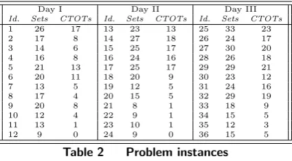
The performance of our pruned dynamic program is illustrated here using complex real world problem instances, covering three days of departure operations at London Heathrow Airport. The instances were first introduced in Atkin et al. (2012) for the pushback time allocation problem. Their characteristics are summarised in Table 2, which shows the number of sets of separation identical aircraft and the number of aircraft with CTOTs. Each instance contains 55 aircraft, of which the first 5 are assumed to be fixed to give a take-off history.
Day I Day II Day III
Id. Sets CTOTs Id. Sets CTOTs Id. Sets CTOTs
1 26 17 13 23 13 25 33 23
2 17 8 14 27 18 26 24 17
3 14 6 15 25 17 27 30 20
4 16 8 16 24 16 28 26 18
5 21 13 17 25 17 29 29 21
6 20 11 18 20 9 30 23 12
7 13 5 19 12 5 31 24 16
8 17 4 20 15 5 32 29 19
9 20 8 21 8 1 33 18 9
10 12 4 22 9 1 34 15 5
11 13 1 23 10 1 35 12 3
[image:27.595.200.413.233.350.2]12 9 0 24 9 0 36 15 5
Table 2 Problem instances
The terminal manoeuvering area around London Heathrow is highly complex. It has ten different standard instrument departure routes in normal use at any time. In addition, up to three different speed classes and five different weight classes have to be considered, resulting in 180 different aircraft types (corresponding to N above) and 32400 possible combinations. This results in a large and complex separation matrix in which triangle inequalities are violated (the separation of subsequent aircraft is influenced by the two most recent ones in general, and more on occasion). A detailed description of the separation requirements at Heathrow Airport is provided in Atkin (2008). It is also obvious from Table 2 that there are more than the usual 3 to 6 different separation classes (as discussed in the arrival scheduling literature) to consider.
relative to the aircraft’s initial position is constrained (i.e., modelling equity as a hard constraint, in addition to the non-linear delay penalty).
Our pruned DP was implemented in Java and all experiments reported in this section were carried out on a single core of an Intel(R) Core(TM)i7 CPU [email protected] desktop PC. Our code was allocated 16GB of RAM and executed on Sun’s Java(TM) Runtime environment (Version 6), on a Windows 7, 64 bit, Enterprise Edition platform. The following parameter settings were used: W1= 100, W2= 10, ω1= 10 ω2= 10000, ω3= 100, ω4= 1000000, α= 1.5, which were taken from Atkin (2008).
4.2. Comparison with previous approaches
As discussed in Section 1, constrained position shifts have been utilised in the past to reduce the problem complexity by limiting the number of positions that each aircraft can take. The problems of such an approach are illustrated in this section.
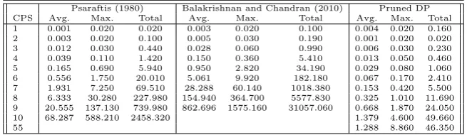
The average, maximum, and total runtime for different values of the constrained position shift and for different previous approaches are listed in Table 3. For instance, the third line in Table 3 for constrained position shift 3 represents the results that were obtained when the maximum number of positions that an aircraft could deviate from its position in the initial sequence was restricted to ±3. All code was implemented in a comparable way and common components were shared between the implementations to make the comparison as fair as possible.
The results show that the computational cost for the approaches introduced by Psaraftis (1980) and Balakrishnan and Chandran (2010) increases rapidly as a function of the constrained position shift. This is in line with the expectations based on their theoretical complexity and with the results in the publications themselves, since they were not designed for such complex problems, relying on having a low number of separation groups. In the case of Balakrishnan and Chandran’s approach, the runs for a constrained position shift of 10 were terminated when our implementation failed to solve the first instance within 12 hours. This was also the case for Psaraftis’ approach when a constrained position shift of 55 was applied (which effectively means that any aircraft could take up any position in the sequence).
CPS
Psaraftis (1980) Balakrishnan and Chandran (2010) Pruned DP
Avg. Max. Total Avg. Max. Total Avg. Max. Total
1 0.001 0.020 0.020 0.003 0.020 0.100 0.004 0.020 0.160
2 0.003 0.020 0.100 0.005 0.030 0.190 0.001 0.020 0.020
3 0.012 0.030 0.440 0.028 0.060 0.990 0.006 0.030 0.230
4 0.039 0.110 1.420 0.150 0.360 5.410 0.013 0.050 0.460
5 0.165 0.690 5.940 0.950 2.820 34.190 0.029 0.080 1.060
6 0.556 1.750 20.010 5.061 9.920 182.180 0.067 0.170 2.410
7 1.931 7.250 69.510 28.288 60.140 1018.380 0.153 0.420 5.500
8 6.333 30.280 227.980 154.940 364.700 5577.830 0.325 1.010 11.690
9 20.555 137.130 739.980 862.696 1575.160 31057.060 0.668 1.870 24.050
10 68.287 588.210 2458.320 1.379 4.600 49.660
[image:28.595.142.470.613.708.2]55 1.288 8.860 46.350
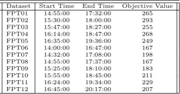
Table 4 lists the results for our approach on the benchmark instances for Milan Airport pro-vided by Furini et al. (2012), containing 60 aircraft each. These instances are freely available from http://www.or.deis.unibo.it/research.html. Furini et al. (2012) do not consider CTOT costs and makespan, and apply a weighted linear delay penalty per aircraft based on its size and fuel con-sumption. I.e., the value ofαin Equation 3 is set to 1 (linear delay cost), the value ofW1 is aircraft dependent and replaced by W1,i, and the value ofW2 is set to 0 (which significantly simplifies the problem).
Furini’s instances were considerably easier to solve than the instances considered for Heathrow Airport. The results in Table 4 were obtained by enabling complete orders, conditional orders, dominance with lower bounding, and insertion dominance. These rules were able to prune the state space sufficiently without the additional computational burden of checking the other pruning rules, and without the need to add additional complexity to the algorithm. The total runtime to solve all problem instances to optimality was 64 milliseconds, or on average 5.3ms per problem instance. This equates to a speedup by a factor of 37170 relative to the runtimes reported in Furini et al. (2012) (which were an average of 197 seconds for heuristically obtained solutions, although we note that the hardware configuration used by Furini et al. (2012) is different from the hardware configuration used to generate the results in this paper). The results reported above for the problem instances from Heathrow and Milan counter the common belief that many real world runway sequencing problems are too complex to solve exactly, despite the difficulty that many algorithms have had in the past.
Dataset Start Time End Time Objective Value
FPT01 14:55:00 17:32:00 265
FPT02 15:30:00 18:00:00 293
FPT03 15:47:00 18:27:00 255
FPT04 16:14:00 18:47:00 268
FPT05 16:35:00 19:36:00 249
FPT06 14:00:00 16:47:00 167
FPT07 14:32:00 17:08:00 198
FPT08 14:55:00 17:37:00 167
FPT09 15:25:00 18:10:00 183
FPT10 15:55:00 18:45:00 211
FPT11 16:24:00 19:34:00 229
[image:29.595.216.397.473.568.2]FPT12 16:45:00 20:17:00 207
Table 4 Optimal results for the benchmark instances introduced by Furini et al. (2012).
4.3. Pruning
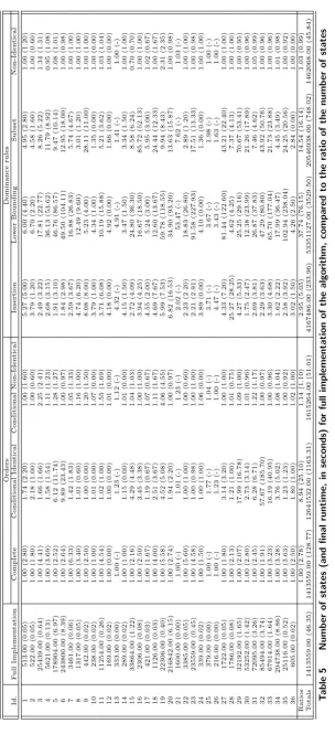
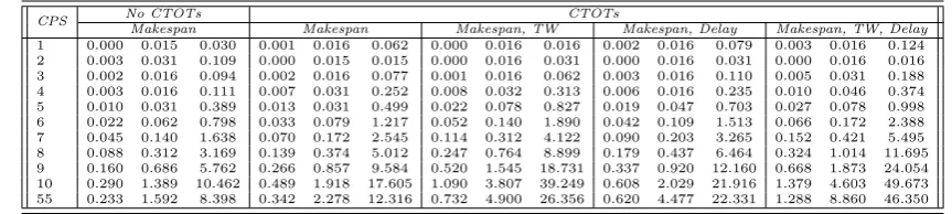
It can be observed from Table 5 that the most efficient principles are dominance with lower bounding, subset dominance, and conditional orders between identical aircraft. These reduced the number of states (or runtimes) by a factor of 37.74 (76.15), 14.54 (16.14), and 8.94 (25.10) respectively. They are followed by insertion dominance, conditional orders between non-identical aircraft, and dominance between non-identical sets, which resulted in a factor of 2.95, 1.14, and 1.03 times fewer states being generated, and speed-ups of a factor of 5.05, 1.10, and 0.99, respectively. The table also shows that conditional orders between identical aircraft covers complete orders, as explained in§3.3.1: exactly the same number of states are generated if the respective rule is disabled. However, the inclusion of complete orders still results in a speed up by a factor of 2.78 by reducing the computational burden. The relative ratio of the state space reduction versus the reduction in runtime illustrates that some principles are more “costly” to implement. However, apart from dominance between non-identical sets, the significant reduction in the number of states always outweighed the additional computational cost of adding the pruning rule to the implementation. Our full implementation is able to generate optimal results in an average runtime of 1.29 seconds per dataset, a maximum runtime of 8.86 seconds, and a total runtime of 46.35 seconds across all 36 instances. We note that no parallelisation of our code was used, however preliminary experiments indicate that further reductions in runtime are possible from parallelisation.
The pruning rules evaluated above exploit three key characteristics that are present in real world instances:
• Aircraft arrive over time and cannot depart before they are ready (insertion dominance, dom-inance with lower bounding)
• Sets of identical aircraft are present (complete orders, conditional orders between identical aircraft)
• The separations are structured (conditional orders between non-identical aircraft and domi-nance between non-identical sets)
These characteristics are expected to be present in the majority of the real world runway sequencing problems, since they are inherent to the core nature of the problem. In the worst case scenario, where every aircraft belongs to a different weight class, and/or speed class, and/or follows a different SID, or all aircraft have a slot, no complete orders can be inferred, and the pruning exploiting conditional orders between identical and non-identical aircraft will become more important. Similarly, if all aircraft are ready at the same time, insertion dominance and dominance with lower bounding will become less efficient, but the other pruning rules will still apply. However, none of these scenarios are likely to occur in practice.