1
Enhanced DBCC for high-speed permanent magnet synchronous
motor drives
M. Tang1, A. Gaeta2, A. Formentini1, K. Ohyama3, P. Zanchetta1, and G. Asher1 1 University of Nottingham, University Park, Nottingham, UK
2 reDrives s.r.l., via Tommaso Fazello 5, Lentini (SR), Italy
3 Fukuoka Institute of Technology, 3-30-1 Wajirohigashi, Higashi-ku, Fukuoka, Japan
Abstract: High bandwidth and accuracy of the current control loop are fundamental requisites when a fast torque response is required or for facilitating the reduction of torque ripple in high performance drives, especially at high speed. One of the most suitable control methods to achieve these goals is dead beat current control (DBCC). Many types of DBCC have been proposed and implemented in literature. This paper proposes a DBCC incorporating two new functionalities. One is a two steps current prediction to improve prediction accuracy when current measurements are taken place before each sampling period; and particularly to reduce the overshoot during transients when mean value is used as current feedback. The second is a novel compensation method for the rotor movement to eliminate offset errors which occur at high speed. Moreover, the dynamic and steady state performance of the proposed DBCC is assessed in simulations. On the basis of the simulation tests, the control parameters are tuned for experiments and the performance of the proposed functionalities are verified. Finally, the advantage of DBCC, compared with a classical dq PI current regulator, is verified in experiments.
1. Introduction
Dead beat current control (DBCC) is categorized as belonging to the predictive control family. It is one of the possible solutions to achieve high-bandwidth and high-accuracy current control loop has been successfully applied for many industrial fields where high performance is required. For examples, for grid generation system in [1]; for multilevel converters in [2]; and for PMSM drives [3-8].It has been for the first time introduced for the control of a PWM inverter used in an uninterruptible power supply (UPS) [9].
Permanent magnet synchronous motors (PMSMs) are widely used in industry applications and different works have been proposed recently in literature [10-14]. In PMSMs, high-frequency electromagnetic torque ripple appears due to the distorted stator flux linkage, variable magnetic reluctance at the stator slots, and imperfect mechanical alignment. Therefore, high-bandwidth and high-accuracy in the current control loop (such as DBCC loop) are the fundamental requisites for facilitating the reduction of torque ripple or when a fast torque response is required in high performance PMSM drives. For example, the basic structure of DBCC for PMSM drives, which is embedded for the compensation of torque harmonics, is proposed and validated with simulation and experimental results in [3, 4]. Authors in [7] propose a DBCC scheme to achieve fast dynamic response.
2
recognised in scientific literature that a current control loop with DBCC has potential to have higher bandwidth compared with a current loop using traditional PI current regulators. However, some of these studies claim that, given its model-based characteristic, deterioration of DBCC performance and eventual instability are possible due to mismatch in model parameter values, un-modelled delays, dead-time effects, and other errors in the model.
Many solutions have been proposed in literature in order to solve this problem. [18] proposes a fast PI controller based on deadbeat algorithm for active power filters. Disturbance observers have been applied to the DBCC for an UPS application to reduce control sensitivity for model uncertainties, parameter mismatches, and noise on sensed variables [19]. For a PMSM drive application, the DBCC combined with classical PI current regulators has been proposed to reduce the current errors that arise due to model mismatches and the non-ideal behaviour of the inverter during steady-state operation in [7]. For a three-phase PWM voltage-source inverter, the DBCC with an adaptive self-tuning load model has been proposed to reduce model mismatches in [20]. A current observer with an adaptive internal model is instead proposed in [21] to compensate system uncertainties of DBCC. A novel neural network-based estimation unit has been proposed to estimate, in real-time, the grid impedance and voltage vector simultaneously in [22]. Although the problem of DBCC has been claimed and many solutions has been proposed, quantitative assessments for its dynamic and steady-state performance on the pre-mentioned uncertainties are not sufficient in existing literature.
3
different from the value measured at the beginning due to rotor movement. Sampling in advance can possibly make the measurements more close to the mean current, therefore, the controller can work to bring the mean current to the demand. 3) Particularly, in case the current is oversampled for reducing noise, and mean current value is calculated as feedback, overshoots in current response may occurs using the traditional DBCC, which can be reduced by properly setting the advanced sampling time.
What is more, the rotor movement is also responsible for an error between the voltage demand and real voltage seen by the motor, consequently steady state error in current response increases as speed increases. Therefore, the rotor movement effect need to be compensated.
Hence, this paper first proposes a DBCC with two new functionalities: One is a two steps current prediction (section 2.1) to improve the accuracy of the current prediction when measurements are taken before the beginning of a period; and particularly in case of the mean current over a period is used as the feedback as in this paper, to cancel the false current error during transients. The other one is a novel compensation method for the rotor movement prediction (section 2.3) to eliminate offset errors which occur at high speed. Second, this paper reveals the influence of parameter mismatch and dead time of the inverter on the band-width, phase shift (delay) and steady state errors by a quantitative performance assessment supported by simulation validation (section 3.1). Third, based on the results of the simulative performance assessment, the parameters are tuned in the experiments and the effectiveness of the two proposed functionalities is verified (section 3.2). Fourth, the classical PI regulator is experimentally compared with DBCC to highlight the advantages of DBCC in terms of bandwidth and delay (section 3.3).
2. Proposed Dead Beat Current Control
This section demonstrates the proposed dead beat current control (DBCC) with two steps current prediction and rotor movement compensation.
The voltage equations of PMSM in a dq reference frame synchronous with the rotor are as follows:
q q e d d d s
d Li
dt di L i R
v (1)
m e d d e q q q s
q Li
dt di L i R
v (2)
Where, vdq are the stator dq axis voltages, idq are the stator dq axis currents, ωe is the rotor electrical
angular speed. Stator inductances Ldq, stator resistance Rs, and permanent magnet flux linkage ψm are
4
The inverter output is updated according to the dq stator voltage references vdqref only at the beginning
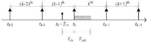
of every sampling period Ts. The timing sequence of DBCC is shown in Fig. 1. For clarity, relevant events
and time durations are drawn only for the kth sampling period.
The principle of DBCC is to calculate the (k+1)th dq voltage references considering time delays Tcs
due to current detection (depending on when exactly the currents are sampled) and the sampling period Ts
of the digital control. A priori knowledge of the motor model is exploited for this purpose. To ensure the availability of samples at the beginning the kth interval, Tcs should be chosen long enough to cover A/D
conversion and transmission times. Full calculations for the DBCC are executed in each sampling period Ts.
Therefore the calculation time Tcal needs to be smaller than Ts. Essentially the required calculations are
performed in three steps as follows:
Fig. 1. Timing sequence of dead beat current control.
2.1. Current Prediction
The calculated (k+1)thdq voltage references will be effectively applied at tk+1, so the initial dq currents
used for calculation should be those at tk+1 and not the ones measured at (tk-Tcs). This to prevent any
overshoot or inaccuracy in the response during transients, since the dq currents at tk+1 can be different from
those measured at t=tk-Tcs as a consequence of the reference voltages applied during the (k-1)th and kth
sampling periods. Since the (k+1)th dq currents are in the future with respect to the kth sampling period (during which calculations are being performed), they must be predicted using the motor model. Considering that the (k-1)th and kthdq voltage references are applied in the time interval [tk-Tcs, tk+1], the predictions must
be performed in two steps. The first current prediction is to predict the dq currents at tk using the (k-1)th dq
reference voltages and the measured dq currents at tk-Tcs. The second current prediction is to predict the dq
currents at tk+1 using the kthdq voltage references and the previously predicted dq currents at tk.
For the first current prediction, the stator voltage references vdqref(k-1) are used instead of the real stator
voltages vdq, since voltage sensor are not usually present in a drive for cost reasons. Please note that vdqref(k
-1) are available during the kth sampling period since calculated during the (k-2)th sampling period. The
vdqref(k-1) and the rotor electrical angular speed ωe(k) are assumed constant in one sampling period. ωe(k)
[image:4.595.168.427.262.338.2]5
is much larger than Ts. Furthermore, under the previous hypotheses, equations (1) and (2) can be rewritten
as:
e
qqd d d s ref
d k Li
dt di L i R k
v 1 (3)
e
d d e
mq q q s ref
q k L i k
dt di L i R k
v 1 (4)
Both sides of equations (3) and (4) are integrated from tk-Tcs to tk.
k L i dtdt di L i R dt k v k cs k k cs k t T
t e q q
d d d s t T t ref d
1
(5)
k L i
k dtdt di L i R dt k v k cs k k cs k t T
t e d d e m
q q q s t T t ref q
1 (6)
The following equations are obtained from (5) and (6) assuming that current profiles are linear. This hypothesis is necessary for avoiding a closed-form solution of the differential equations (5) and (6). Although the hypothesis will not be true once the motor starts rotating and will even cause steady state errors in current responses, this steady state error can be cancelled by the rotor movement compensation method proposed in 2.3. The hypothesis may also be wrong if Tsis not sufficiently small (10 times) compared with
the electrical time constant of the motor. In the case study of this paper, Ts is 52 times smaller than the
electrical time constant.
e
q cs
q
k q k cs
cs k d d cs s k d d cs s ref d
cs i t i t T
T L k T t i L T R t i L T R k v
T
2 2 2
1 (7)
m cse cs k d k d cs d e cs k q q cs s k q q cs s ref q cs T k T t i t i T L k T t i L T R t i L T R k v T 2 2 2 1 (8)
The kth dq currents are detected at tk-Tcs. Therefore the following assumptions for the measured
currents are used to execute the first current prediction.
mea
d d k cs
i k i t T (9)
q
k cs
mea
q k i t T
i (10)
Therefore the estimated dq currents idqpre(k) of the first current prediction are derived from equations
6
2 32 1 2 2 2 4 3 1 2 2 3 2 1 2 1 a a k a k T L k i k T L k i a a a k k v k T L k v T a k i e e m cs q mea q e cs q mea d e ref q e cs q ref d cs pre d (11)
2 32 1 2 5 2 1 2 2 2 2 1 1 2 a a k a k T a k i a a a k k i k T L k v T a k v k T L k i e e m cs mea q e mea d e cs d ref q cs ref d e cs d pre
q
(12) Where, 4 2 1 cs q dLT
L
a , d
cs sT L R
a
2
2 , q
cs sT L R
a
2
3 , d
cs sT L R
a
2
4 , q
cs s
L T R
a
2
5
In the experimental tests of this paper, the currents are sampled at a rate of 15MHz on the FPGA, and the mean current value over one sampling period is fed back to the controller so that it can bring the mean currents to its reference in steady state. As a consequence, to avoid the false current error during transients, it is necessary to use the first prediction to predict the real current at the end of each sampling interval from the mean value. In such case, the mean current can be assumed to be the same as the current measured at the middle of the sampling interval idq(tk-Ts/2) since a linear profile of current is assumed. Hence, only for taking
into account the particular way the current are measured in the experimental system, Tcs=Ts/2 in this paper.
The second current prediction predicts the dq currents at tk+1using the kth voltage referenceand the dq
current at tk obtained from the first current prediction. For the second current prediction, the stator voltage
references vdqref(k) are used instead of the real stator voltages vdq. Again, the vdqref(k) are available during the
kth sampling period since calculated during the (k-1)th sampling period and the vdqref(k) and the rotor electrical
angular speed ωe(k) are assumed constant during the sampling period.
e
q qd d d s ref
d k Li
dt di L i R k
v (13)
e
d d e
mq q q s ref
q k L i k
dt di L i R k
v (14)
Both sides of equations (13) and (14) are integrated from tk to tk+1.
k L i dtdt di L i R dt k v k k k k t
t e qq
d d d s t t ref d
1 1
(15)
k L i
k dtdt di L i R dt k v k k k k t
t e d d e m
q q q s t t ref q
1 1 7
The following equations are obtained from (15) and (16).
q
k q k
s q e k d d s s k d d s s ref d
s i t i t
T L k t i L T R t i L T R k v
T
1 1
2 2
2
(17)
d
k d
k
e
m ss d e k q q s s k q q s s ref q
s i t i t k T
T L k t i L T R t i L T R k v
T
1 1
2 2
2 (18)
Once again the following relations are considered:
t
i
k
i
d k
dpre (19)
t i
kiq k qpre (20)
Therefore the estimated dq currents of the second current prediction are derived from the equations (17-20).
2 32 1 2 2 2 4 3 2 1 2 3 2 2 1 b b k b k T L k i k T L k i b b k b k v k T L k v T b k i e e m s q pre q e s q pre d e ref q e s q ref d s pre d (21)
2 32 1 2 5 2 1 2 2 2 2 2 1 b b k b k T b k i b b b k k i k T L k v T b k v k T L k i e e m s pre q e pre d e s d ref q s ref d e s d pre q (22) Where, 4 2 1 s q dL T L
b , b RsTs Ld
2
2 , q
s sT L R
b
2
3 , d
s sT L R
b
2
4 , q
s sT L R
b
2
5
2.2. Voltage References with Current Predictions
The (k+1)th dq stator voltage references vdqref(k+1), applied in the period tk+1 to tk+2, are calculated
from the predicted dq currents at tk+1, idqpre(k+1), and dq current references at tk, idqref(k), as in the following.
Again, the current profiles are assumed to be linear in order to simplify the differential terms.
i
k i
k
L
k i kT L k i R k
v dref dpre q e qref
s d ref d s ref
d 1 1 (23)
i
k i
k
L
k i
k
k T L k i R kv qref qpre d e dref m e
s q ref q s ref
q 1 1 (24)
In this case, the kthdq current references will effectively set the dq currents at tk+2, and consequently
8
to predict the (k+2)th dq current references starting from the kth ones which are known only when the calculations are performed. However such a prediction is typically done by interpolation and is effective only in case of periodic references. When the (k+2)th dq current references, idqref(k+2), are available, the
vdqref(k+1) can be calculated from the idqpre(k+1) and the idqref(k+2) as described by the following equations:
1
2
i
k2
i
k1
L
k i k2
T L k
i R k
v dref dpre q e qref
s d ref
d s ref
d (25)
i
k
i
k
L
k i
k
kT L k
i R k
v qref qpre d e dref m e
s q ref
q s ref
q 1 2 2 1 2 (26)
For emphasizing the intrinsic delay of the DBCC, no prediction for the reference currents is performed in this paper.
2.3. Rotor Movement Compensation
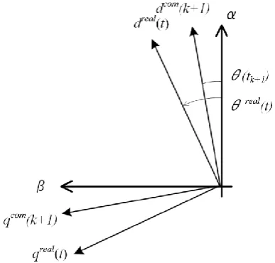
The vdqref(k+1) are maintained for the whole (k+1)th sampling period; however during that period the
rotor moves and the real dq voltages vdqreal(t) applied to it are different from the vdqref(k+1). Especially at
high speed, the rotor movement in a sampling period is not negligible. Consequently, the non-constant real voltage vdqreal(t) is responsible for the nonlinear current profile, and the difference between the real average
voltages vdqavg(k+1) applied to the rotor during the (k+1)th sampling period and the reference voltages
vdqref(k+1) is responsible for a steady state error/offset between the reference currents idqref(k+2) and the actual
currents at tk+2. In order to avoid this issue, the novel technique proposed in this paper is to apply the
compensated dq voltage references vdqcom(k+1) at tk+1 so that the average dq voltages vdqavg(k+1) effectively
applied to the motor during the (k+1)th sampling period are equal to the v
dqref(k+1). The relationships between
the instantaneous vdqreal(t) and the vdqcom(k+1) are described by the following equations with reference to the
dq reference frame taking into account the rotor movement in Fig.2.
cos
( 1)
1
sin
( 1)
1
real real com real com
d k d k q
v t t t v k t t v k (27)
sin
( 1)
1
cos
( 1)
1
real real com real com
q k d k q
v t
t
t v k
t
t v k (28)The term
real
( 1)
k
t t
represents the difference between the instantaneous position and the initial position at the beginning of each sampling period. Therefore
real
t (tk1)
can be replaced by
e k t
. Both sides of (27) and (28) are integrated from 0 to Ts to obtain:
s
s
Ts
com
q e
T com
d e
T real d avg
d
sv k v t dt k t v k dt k t v k dt
T
0 0
0 cos 1 sin 1
1 (29)
s
s
Ts
com
q e
T com
d e
T real q avg
q
sv k v t dt k t v k dt k t v k dt
T
0 0
0 sin ( ) 1 cos ( ) 1
9
Fig. 2. dq reference frame for rotor movement.
The average voltages vdqavg(k+1), compensated voltages vdqcom(k+1) and the rotor angular speed ωe(k)
are assumed constant for the integration interval. By imposing that the applied vdqavg(k+1) equals to
vdqref(k+1), the following equations are obtained from (29) and (30):
1
sin
1
cos
1v
k1
k T k k v k T k k v
T qcom
e s e com d e s e ref d s
(31)
1
cos
1
1
sin
v
k1
k T k k v k T k k v
T qcom
e s e com d e s e ref q s
(32) Therefore the vdqcom(k+1) are derived from (31) and (32).
ref ref
s e s e d s e s e q
com
d 2 2
e s e s
T sin k T k v k 1 T cos k T 1 k v k 1
v k 1
sin k T cos k T 1
(33)
22 1 cos sin 1 sin 1 1 cos 1 s e s e ref q e e s ref d e s e s com q T k T k k v k T k T k v k T k T k v (34)
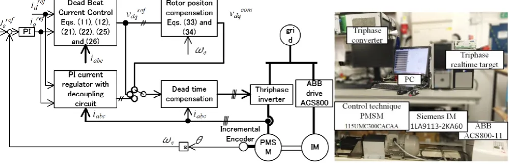
A scheme of the implemented control can be seen in Fig. 3.
3. Proposed control strategy Assessment with Simulation and Experimental tests
[image:9.595.200.394.57.242.2]10
Simulation tests are carried out using MATLAB Simulink. The simulation model includes the permanent magnet synchronous motor, the controller, and the three phase inverter which is modelled considering a dead time related voltage error of which the polarity varies according to the polarity of the phase currents. The experimental test rig is set up as in Fig.3 where a DBCC and a PI controller are both implemented for comparison. The current control schemes can be switched over in the software easily. The speed control loop is used to keep the rotor speed constant or generate the high frequency sinusoidal signal in the iqref for test reasons. A “Triphase” evaluation system, composed by an inverter and a
[image:10.595.40.476.301.441.2]real-time control platform is used in the experimental tests. The program in the FPGA inside the Triphase Realtime Target can be compiled directly using Matlab Simulink, and the Triphase converter is controlled by the Realtime Target to drive a Control Technique PMSM (115UMC300) with parameters as shown in Table 1. A Siemens induction motor (IM) (1LA9113) is used as load.
Table 1 Motor Parameters
Name of parameter Value Name of parameter Value
Rated power 2.54 [kW] d axis stator inductances Ld 4.5 [mH]
Rated speed 3000 [min-1] q axis stator inductances L
q 7.4 [mH]
Rated torque 9.4 [Nm] Stator resistance Rs 1.4 [Ω]
Rated voltage 400 [V] Magnetic flux linkage Fm 0.237 [Wb]
Rated current 5.9 [A] Inertia 0.007 [kgm2]
Number of pole pairs 3
Fig. 3. Experimental system.
3.1. Performance Assessment
[image:10.595.53.553.487.650.2]11
PMSMs, it would be ideal if the DBCC could track a wide frequency range of sinusoidal references with no attenuation, smallest possible phase shift and no offset in the average value. In this section, the Bode diagram is mapped in simulation to verify bandwidth, amplitude and phase response of DBCC, while, the steady state error in step response is mapped to verify the offset. In summary, the following results in 3.1.1 and 3.1.2 show that the dynamic performance (amplitude and delay) is affected mainly by detuned inductances while the steady state performance by the detuned magnetic flux.
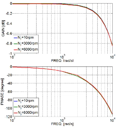
3.1.1 Bode Diagram
For mapping Bode diagrams as shown in Fig.4, the reference current iqref is set to be a sinusoidal
signal with bias of 8.34A (the rated current), the motor speed Nr is set to be constant, and the amplification
or attenuation in the magnitude of the response as well as the phase shift are calculated. This procedure has been repeated iteratively for current references of different frequencies and with different motor speed, different motor parameter detuned. For example, Ldest/Ld = 0.5 in Fig.4b means that Ldest (estimated in the
control) is 50% of Ld (real value in the motor). It is also to be noticed that the results in Fig.4e for 10000rad/s
and 5000rad/s are confirmed by the experimental results shown in Fig.9a and Fig.10a 10c in section 3.3. Regarding bandwidth and amplitude response, the high bandwidth characteristic of DBCC is reliably maintained for varying speed Nr (Fig.4e) and for parameter mismatch of the magnetic flux Fm (Fig.4d). Also,
since idref = 0A, the control performance is reliable with detuned Ld (Fig.4b). A mismatch of Rs (Fig.4a) not
necessarily reduces the bandwidth, but may result in an increase (when Rsest>Rs) or a decrease (when Rsest<Rs)
in the amplitude of iq. In case of detuned Lq (Fig.4c), the bandwidth of DBCC can be significantly reduced
when Lqest<Lq; when Lqest>Lq the amplification introduced at high frequencies may bring challenges for the
stability of the iq control loop. It can thus be suggested, during the design of DBCC needs, to consider a
smaller dq axis inductances for stability reason, but not too small to avoid sacrificing the bandwidth.
Before discussing the phase response, it would be necessary to define the smallest possible phase shift
for DBCC. Theoretically, the reference current can be achieved only 2Ts after the reference change has been
detected by the control or even longer (An example is given in Fig.7cd in 3.2.1) depending on the demanded current change and the available DC bus voltage. As a result, when operating below the voltage limitation, the phase shift of a signal is proportional to its frequency and equals to the frequency multiplied by 2Ts. This
calculation is supported by almost all the phase plots in Fig.4 apart from the case of the detuned Lq (Fig.4c).
Considering the worst case when Lqest=0.5Lq in Fig.4c, the phase lagging for 5000rad/s is 85.7°(=1.496rad)
12
however, no significant influence is noticed when the detuned inductance is within a reasonable range (50% to 150% of the real value).
a b
13
e
Fig. 4. Simulation results of bode diagrams of q axis current control loop ( idref = 0A, bias of iqref= 8.34A,Ts = 100µs) a Rsest = (0.5~1.5)Rs, Nr = 3000 rpm
b Ldest = (0.5~1.5)Ld, Nr = 3000 rpm
c Lqest = (0.5~1.5)Lq, Nr = 3000 rpm
d Fmest = (0.5~1.5)Fm, Nr = 3000 rpm
e Nr = 10, 3000, 6000rpm
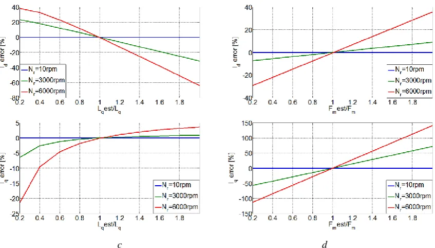
3.1.2 Steady State Error Plot
For mapping the steady state error plots as shown in Fig.5, both the reference current idqref and motor
speed Nr are set to be constant and the error at steady state in the response current idq are calculated using
the equations (35)(36). Again, the procedure is repeated for different settings of reference current value, motor speed, detuned motor parameter, and inverter dead time. Fig.6 shows the influence of switching devices dead time on the steady state errors in current responses using DBCC. The sampling frequency of DBCC is fixed at 10kHz while the dead time varies from 0μs to 10μs.
2 2 100
ref q ref
d
ref d d d
i i
i i i
for error state
Steady (35)
2 2 100ref
q q
q
ref ref
d q
i i Steady state error for i
i i
(36)
[image:13.595.185.409.57.310.2]14
that the steady state offset of DBCC is the most sensitive to the magnetic flux Fm and the dead time of
inverter. Although the dead time effect can be compensated by many existing compensation methods[23], considering the results shown in Fig.4e it may also be possible to compensate the remaining steady state errors at a certain speed (non-zero) by tuning the estimated Fmin the control since the performance of the
DBCC will not be influenced by Fm.
Another interesting finding is that the results in Fig.5 and 6 may give a clue for offline tuning of the machine parameters. For example, through increasing the estimated Fm, Ld, and Rs or decreasing the
estimated Lq in the controller, the d axis current id can be increased; Similarly, the q axis current iq can be
increased by increasing the estimated Fm, Lq, and Rsor decreasing the estimated Ldin the controller; As the
dead time increases, the steady state error positively increases in id and negatively increases in iq.
15 c d
Fig. 5. Simulation results of steady state current errors of DBCC due to parameter detuning (idref =0A, iqref=8.34A) a Rsest=(0.2~2)Rs, Nr = 0~6000rpm
b Ldest=(0.2~2)Ld, Nr = 0~6000rpm
c Lqest=(0.2~2)Lq, Nr = 0~6000rpm
d Fmest=(0.2~2)Fm, Nr = 0~6000rpm
a b
Fig. 6. Simulation results of steady state current errors of DBCC due to dead time (idref=0A, Nr=3000rpm) a iqref=0.8A
b iqref=8.34A
3.2. Effectiveness of the Proposed DBCC
Turning now to the experimental tests of the proposed DBCC with two steps current prediction and rotor movement compensation, the machine parameters are tuned based on the findings in 3.1.2 and the results are as shown in Table 1. It is also to be noticed that the IGBT voltage drops and dead time of inverter is compensated by using a lookup table as demonstrated in [23].
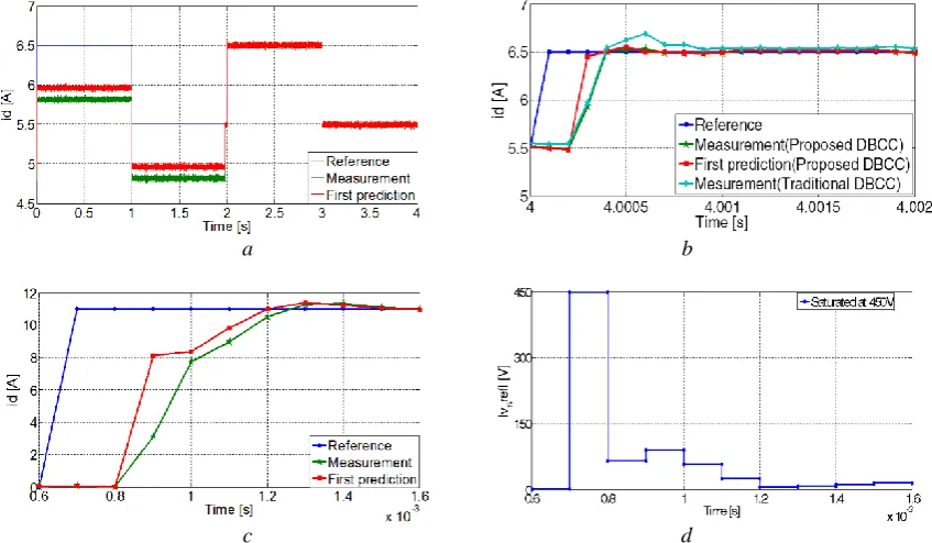
3.2.1 Two Steps Prediction and Operating at Physical Limit
[image:15.595.81.505.56.297.2] [image:15.595.73.523.383.525.2]16
are shown in Fig.7bc. In both cases, the rectangular current references are generated by the idcurrent loop.
Moreover, the current responses of the same rectangular reference using the proposed DBCC (with two steps current prediction) and the traditional DBCC (with only one step prediction) are compared in Fig.7b to show the necessity of having two steps current prediction instead of one.
It can be seen from Fig.7a that with properly tuned parameters and properly compensated inverter nonlinearities, the proposed DBCC can achieve zero steady state error in the response.
By comparing the measured current (green) and the first prediction current (red) in Fig.7b, it can be seen that the first prediction current reaches its demand after 2Ts and the measurement current, which is a
mean current, reaches the demand after 3Ts. By comparing the measured current (green) for the proposed
[image:16.595.85.509.392.639.2]DBCC and the measured current (light blue) for the traditional DBCC (the first prediction is removed), it can be seen that an overshoot of 18.6% occurs without the first prediction. These results confirm the necessity of the first prediction as discussed in 2.1. The first prediction works to predict the real instantaneous current at 4.0003s so that the controller can have a fairly accurate judgement of whether the demand has been achieved or not.
Fig.7c shows that a longer settling time (as discussed in 3.1.1) of 5Ts is required for DBCC to achieve
a current step of 11A with the peak value of the three-phase voltage limited at 450V.
a b
c d
Fig. 7. Experimental results of rectangular current responses of DBCC
a With the proposed DBCC, idref is 0.5Hz (the inverter compensation is activated around 2s)
b Comparison between the proposed DBCC and the traditional DBCC (without the first prediction), idref is 0.5Hz
c With the proposed DBCC and inverter compensation, idref steps from 0A to 11A (above voltage limitation)
17
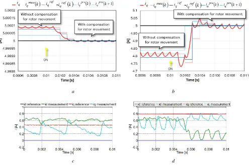
3.2.2 Rotor Movement Compensation
Figs.8a and 8b show the effects of the rotor movement compensation in simulation, which starts at 0.01s. The voltage references maintain a maximum two sampling time delays including a calculation step. Therefore it is shown that the offsets start to decrease after 2 sampling periods. Similarly, the experimental results in Figs.8c and 8d confirm the effectiveness of the proposed rotor movement compensation. The steady errors are calculated by equations (35) and (36), where mean values are used for id and iq in the
equations. By adding the proposed rotor position compensation, at 1000rpm, the steady state error in id
reduces from 132% to 122%, while the error in iq reduces slightly from -19% to -17%. Meanwhile, at
2930rpm, the steady state error in id reduces significantly from 81% to 27%, while the error in iq reduces by
half from -37% to -18%. It is obvious from both the simulation and the experiment that the rotor position compensation works for all speeds, but is much more effective at high speed as discussed in 2.3. Unfortunately, due to the parameter variations in motor and imperfect inverter compensation, the rotor position compensation method cannot remove all steady state errors in the experiments.
a b
c d
Fig. 8. Steady state current errors due to rotor movement (iqref=5A) a Simulation results iqref=5A, Nr=100rpm;
b Simulation results iqref=5A,Nr=5000rpm
c Experimental results idref =0A, Nrref= 1000rpm, the rotor position compensation is activated at 0.005s
[image:17.595.52.548.323.654.2]18
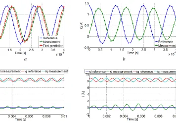
3.3. Comparison Between DBCC and PI
[image:18.595.77.506.284.409.2]Furthermore, the performance of DBCC is compared with that of a conventional dq PI current regulator with a decoupling circuit. The bandwidth of the dq PI control loop used for comparison is designed to be around 900Hz with classical SISO control design methods. The no load test results for the current responses to a very high frequency current reference (10000rad/s) are shown in Fig.9. The no load and full load test results for the current responses to a high frequency current reference (5000rad/s) are shown in Fig.10. The full load operation is tested using a commercial drive (ABB ACS800-11). The ABB drive is operated under a speed control mode. The rotor speed is kept at 2500rpm, and the iqref is set at the rated value
of 8.34A. No tests are performed for frequencies higher than 10000rad/s since it is unlikely to have speed ripple at such high frequencies due to the low-pass filtering effect of the mechanical system.
a b
Fig. 9. Experimental results of current responses for a very high frequency (Nrref= 2930+30sin(10000t) rpm, idref =0A) a No load, DBCC
b No load, PI
[image:18.595.146.503.455.705.2]19 c d
Fig. 10. Experimental results of current responses for a high frequency (idref =0A) a No load, DBCC Nrref= 2930+30sin(5000t) rpm
b No load, PI Nrref= 2930+30sin(5000t) rpm
c Full load, DBCC Nr= 2500 rpm, iqref =8.34+0.5sin(5000t) A
d Full load, PI Nr= 2500 rpm, iqref =8.34+0.5sin(5000t) A
For DBCC, it can be seen from Fig.9a that the first current prediction is able to track the reference after two samples which is the smallest possible delay as discussed in 3.1.1. The phase shift is 115° (=2rad) which is exactly 10000rad/s multiplied by 2Ts (=0.0002s). This last result confirms the phase plot in Fig.4e.
Additionally, the attenuation is about -0.55dB. This is reasonably close to the simulated result for 10000rad/s (-0.8dB) as shown in Fig.4e. Furthermore, the attenuation (-0.25dB) and phase shift (57°) for 5000rad/s in Fig.4e is also supported by the experimental results as shown in Fig.10ac, where the phase lag of the first prediction current equals to 5000rad/s multiplied by 2Ts (=0.0002s), thus 57°, and the attenuation is about
-0.61dB.
When using a traditional PI regulator, as can be seen from Fig.9b and Fig.10bd, the phase lag for 10000rad/s is about 200° (=3.5rad), which can be also represented by a delay time of 350μs (=3.5rad divided by 10000rad/s); the phase lag for 5000rad/s is about 133° (=2.3rad), which is equivalent to a delay time of 460μs. Moreover, the signal is attenuated of -9.7dB (out of bandwidth) at 10000rad/s and of -1.4dB at 5000rad/s. Although the bandwidth and response can be improved by a better designed PI, the fact that the delay of the PI control loop varies with frequency cannot be changed.
It is worth noting that, in the no load test, the PMSM is driven under speed control mode, while in the full load test, it is under current or torque control mode. Practically, depending on specific applications, PMSM can also be operating under position control mode. Cascaded outer loops are added when under speed or position control modes. These experimental tests confirm the same behavior of the inner current loop under different control modes. When choosing between DBCC and PI, it is worth to consider if only inner loop is used (i.e. in torque control mode), or outer loops are used (i.e. in speed and position control mode) since the steady state error of current response can matters more in the toque control, and delay of the current loop may be more important when outer loop are present.
20 4. Conclusions
This paper has presented an improved high performance DBCC including two steps current predictions and a novel rotor movement compensation method for PMSM motor drives and has provided a detailed performance assessment under different operating conditions supported by simulation and experimental results. The two steps current prediction is necessary to improve the accuracy of the current prediction during transients. The rotor movement compensation is particular useful at high speed for reducing steady state errors in the current response due to the rotor position changing during each sampling period. Bode diagrams of the DBCC controlled system show that the bandwidth and phase response characteristic of DBCC are reasonably maintained even in the case of parameter detuning. Steady state analysis of the DBCC is useful in the design phase in order to indicate the current responses obtained with mismatched parameters, so to facilitate control tuning. The comparison between DBCC and a traditional PI regulator in dq reference frame with decoupling circuit in terms of control dynamics and steady state characteristics shows the main convenience of using DBCC, besides faster dynamics, is to have the fixed delay time for different frequencies. Therefore, the delay introduced by the DBCC loop can be compensated from the outer loop easily.
5. Acknowledgments
This research has been carried out within the Shenzhen Best Motion Technology innovation centre at the University of Nottingham. The authors wish to acknowledge the company financial support and motivation.
6. References
[1] Chen, Y., Luo, A., Shuai, Z., et al.: 'Robust Predictive Dual-Loop Control Strategy with Reactive Power
Compensation for Single-Phase Grid-Connected Distributed Generation System', Power Electronics, IET, 2013, 6,
(7), pp. 1320-1328
[2] Can, W. and Boon-Teck, O.: 'Incorporating Deadbeat and Low-Frequency Harmonic Elimination in Modular
Multilevel Converters', Generation, Transmission & Distribution, IET, 2015, 9, (4), pp. 369-378
[3] Holtz, J. and Springob, L.: 'Identification and Compensation of Torque Ripple in High-Precision Permanent
Magnet Motor Drives', Industrial Electronics, IEEE Transactions on, 1996, 43, (2), pp. 309-320
[4] Springob, L. and Holtz, J.: 'High-Bandwidth Current Control for Torque-Ripple Compensation in Pm
Synchronous Machines', Industrial Electronics, IEEE Transactions on, 1998, 45, (5), pp. 713-721
[5] Sozer, Y., Torrey, D.A., and Mese, E.: 'Adaptive Predictive Current Control Technique for Permanent Magnet
21
[6] Shaowei, W. and Wan, S.: 'Full Digital Deadbeat Speed Control for Permanent Magnet Synchronous Motor with
Load Compensation', Power Electronics, IET, 2013, 6, (4), pp. 634-641
[7] Wipasuramonton, P., Zhu, Z.Q., and Howe, D.: 'Predictive Current Control with Current-Error Correction for
Pm Brushless Ac Drives', Industry Applications, IEEE Transactions on, 2006, 42, (4), pp. 1071-1079
[8] Hyung-Tae, M., Hyun-Soo, K., and Myung-Joong, Y.: 'A Discrete-Time Predictive Current Control for Pmsm',
Power Electronics, IEEE Transactions on, 2003, 18, (1), pp. 464-472
[9] Kawabata, T., Miyashita, T., and Yamamoto, Y.: 'Dead Beat Control of Three Phase Pwm Inverter', Power
Electronics, IEEE Transactions on, 1990, 5, (1), pp. 21-28
[10] Calvini, M., Carpita, M., Formentini, A., et al.: 'Pso-Based Self-Commissioning of Electrical Motor Drives',
IEEE Trans. Ind. Electron., 2015, 62, (2), pp. 768-776
[11] Formentini, A., de Lillo, L., Marchesoni, M., et al.: 'A New Mains Voltage Observer for Pmsm Drives Fed by
Matrix Converters', in, EPE, 2014
[12] Formentini, A., Trentin, A., Marchesoni, M., et al.: 'Speed Finite Control Set Model Predictive Control of a
Pmsm Fed by Matrix Converter', IEEE Trans. Ind. Electron., 2015, 62, (11), pp. 6786-6796
[13] Rovere, L., Formentini, A., Gaeta, A., et al.: 'Sensorless Finite Control Set Model Predictive Control for Ipmsm
Drives', IEEE Trans. Ind. Electron., 2016, PP, (99), pp. 1-1
[14] Formentini, A., Oliveri, A., Marchesoni, M., et al.: 'A Switched Predictive Controller for an Electrical
Powertrain System with Backlash', IEEE Trans. Power Electron., 2016, PP, (99), pp. 1-1
[15] Cortes, P., Kazmierkowski, M.P., Kennel, R.M., et al.: 'Predictive Control in Power Electronics and Drives',
Industrial Electronics, IEEE Transactions on, 2008, 55, (12), pp. 4312-4324
[16] Morel, F., Xuefang, L.-S., Retif, J.M., et al.: 'A Comparative Study of Predictive Current Control Schemes for a
Permanent-Magnet Synchronous Machine Drive', Industrial Electronics, IEEE Transactions on, 2009, 56, (7), pp.
2715-2728
[17] Preindl, M. and Bolognani, S.: 'Comparison of Direct and Pwm Model Predictive Control for Power Electronic and Drive Systems', in, Applied Power Electronics Conference and Exposition (APEC), 2013 Twenty-Eighth Annual IEEE, 2013
[18] Zhou, Z. and Liu, Y.: 'Time Delay Compensation-Based Fast Current Controller for Active Power Filters',
Power Electronics, IET, 2012, 5, (7), pp. 1164-1174
[19] Mattavelli, P.: 'An Improved Deadbeat Control for Ups Using Disturbance Observers', Industrial Electronics,
IEEE Transactions on, 2005, 52, (1), pp. 206-212
[20] Mohamed, Y.A.R.I. and El-Saadany, E.F.: 'An Improved Deadbeat Current Control Scheme with a Novel Adaptive Self-Tuning Load Model for a Three-Phase Pwm Voltage-Source Inverter', Industrial Electronics, IEEE
Transactions on, 2007, 54, (2), pp. 747-759
[21] Mohamed, Y.A.R.I. and El-Saadany, E.F.: 'Robust High Bandwidth Discrete-Time Predictive Current Control with Predictive Internal Model-a Unified Approach for Voltage-Source Pwm Converters', Power Electronics, IEEE
22
[22] Mohamed, Y.A.R. and El-Saadany, E.F.: 'Adaptive Discrete-Time Grid-Voltage Sensorless Interfacing Scheme for Grid-Connected Dg-Inverters Based on Neural-Network Identification and Deadbeat Current Regulation', Power
Electronics, IEEE Transactions on, 2008, 23, (1), pp. 308-321
[23] Gaeta, A., Zanchetta, P., Tinazzi, F., et al.: 'Advanced Self-Commissioning and Feed-Forward Compensation