Graph clustering, variational image segmentation methods and Hough transform scale detection for object measurement in images

(will be inserted by the editor)

Graph clustering, variational image segmentation methods and

Hough transform scale detection for object measurement

in images

Luca Calatroni · Yves van Gennip · Carola-Bibiane Sch¨onlieb · Hannah M. Rowland · Arjuna Flenner

Received: date / Accepted: date

Abstract We consider the problem of scale detection in images where a region of interest is present together with a measurement tool (e.g. a ruler). For the seg-mentation part, we focus on the graph based method presented in [10] which reinterprets classical continuous Ginzburg-Landau minimisation models in a totally dis-crete framework. To overcome the numerical difficulties due to the large size of the images considered we use matrix completion and splitting techniques. The scale on the measurement tool is detected via a Hough trans-form based algorithm. The method is then applied to some measurement tasks arising in real-world applica-tions such as zoology, medicine and archaeology.

L. Calatroni

MIDA group, Dipartimento di Matematica, Universit´a degli studi di Genova, Via Dodecaneso 35, 16146, Italy.

E-mail: [email protected]

Y. van Gennip

School of Mathematical Sciences, The University of Notting-ham University Park, NG7 2RD, NottingNotting-ham, UK.

E-mail: [email protected]

C.-B. Sch¨onlieb,

Department of Applied Mathematics and Theoretical Physics (DAMTP), University of Cambridge, Wilberforce Road, CB3 0WA, Cambridge, UK.

E-mail: [email protected]

H. M. Rowland

Department of Zoology, University of Cambridge, Downing Street, CB2 3EJ, Cambridge, UK;

Institute of Zoology, Zoological Society of London, Regents Park, NW1 4RY, London, UK.

E-mail: [email protected]

A. Flenner

Image and Signal Processing Branch, NAVAIR, 1 Adminis-trative Circle, China Lake CA, USA.

E-mail: [email protected]

Keywords Graph clustering · Discrete Ginzburg-Landau functional · Image segmentation · Scale detection·Hough transform.

1 Introduction

The non-smoothness of most of the segmentation energies renders their numerical minimisation usually difficult. In the case of the Mumford-Shah segmentation model the numerical realisation is additionally compli-cated by its dependency on the image function as well as the object contour. To overcome this, several regu-larisation methods and approximations have been pro-posed in the literature, e.g. [4, 11, 12, 68] for Mumford-Shah segmentation. In the context of TV based seg-mentation models the Ginzburg-Landau functional has an important role. Originally considered for the mod-elling of physical phenomena such as phase transition and phase separation (cf. [13] for a survey on the topics) it is used in imaging for approximating the TV energy. Some examples of the use of this functional in the con-text of image processing are [27, 25, 26], which relate to previous works by Ambrosio and Tortorelli on diffuse interface approximation models [5, 4].

Such variational methods for image segmentation have been extensively studied from an analytical point of view and the segmentation is usually robust and com-putationally efficient. However, variational image seg-mentation as described above still faces many problems in the presence of low contrast and the absence of clear boundaries separating regions. Their main drawback is that they are limited to image features which can be mathematically formalised (e.g. in terms of an image gradient) and encoded within a segmentation energy. In recent years dictionary based methods have become more and more popular in the image processing commu-nity, complementing more classical variational segmen-tation methods. By learning the distinctive features of the region to be segmented from examples provided by the user, these methods are able to segment the desired regions in the image correctly.

In this work, we consider the method proposed in [10, 29, 44, 43] for image segmentation and labelling. This approach goes beyond the standard variational approach in two respects. Firstly, the model is set up in the purely discrete framework of graphs. This is rather unusual for variational models where one normally considers func-tionals and function spaces defined on subdomains of_R2 in order to exploit properties and tools from convex and functional analysis and calculus of variations. Secondly, the new framework allows for more flexibility in terms of the features considered. Additional features like tex-ture, light intensity or others, can be considered as well without encoding them in the function space or the reg-ularity of the functions. Due to the possibly very large size of the image (nowadays of the order of megapixel for professional cameras) and the large number of fea-tures considered, the construction of the problem may be computationally expensive and often requires

reduc-tion techniques [54, 53, 28]. In several papers (see, e.g., [61, 63, 34]) the segmentation problem was rephrased in the graph framework by means of the graph cut ob-jective function. Follow-up works on the use of graph-based approaches are, for instance, [45, 46] where an iterative application of heat diffusion and threshold-ing, also known as the Merriman-Bence-Osher (MBO) method [47] is discussed for binary image labelling, and [37] where the Mumford-Shah model is reinterpreted in a graph setting.

In this paper, we also address the problem of de-tection of objects with geometrical properties that are a priori known. An example is the detection of lines and circles. These objects can be identified by mapping them onto an auxiliary space where relevant geometri-cal properties (such as linear alignment and roundness) are represented as peaks of specific auxiliary functions. In this work, we use the Hough transform [36] to detect measurement tools (rulers, concentric circles of fixed radii) with the intent of providing quantitative, scale-independent measurements of the region segmented by one of the techniques described above. In this way, an absolute measurement of the region of interest in the image is possible, independent of the scale of the im-age, which could depend, for instance, on the distance of the objective to the camera.

inmm2using IMAGEJ software [2]. But none of these three papers provide methods of how the measurement was actually achieved, e.g., whether patches were delin-eated or roughly estimated with a simple shape. Most recently Moreno et al. [51] analysed digital photos of forehead patches with Adobe PhotoShop CS version 11.0. relating the distance of 1mmon the ruler to num-ber of pixels, and used this to estimate length. Zooming to 400% and using the paintbrush tool with 100% hard-ness and 25% spacing the authors delineate the patch and measure the area of the white areas on forehead. While this is the best measurement method to date, it still is subject to human measurement error and sub-jective assessment of patch boundaries. We report some segmentation results obtained by manual selection and polygon fitting in Figure 2. In this manuscript we use a mathematically robust approach to segment the blaze independently to provide an accurate measurement of forehead patch area.

(a) (b)

(c) (d)

Fig. 1: The blaze segmentation and measurement prob-lem: pictures are taken at different distances, thus re-quiring a measurement tool.

A similar challenge can be encountered in medical applications monitoring and quantifying the evolution of skin moles for early diagnosis of melanoma (skin can-cer). A normally user-dependent measurement of the mole is performed using a ruler located next to it. A pic-ture is then taken and used for fupic-ture comparisons and follow-up, see Figure 3 and compare [18, 1] for previ-ous attempts of automatic detection of melanomas. For

(a) Magic wand

(b) Trapezium fitting

Fig. 2: Flycatcher blaze segmentation of the images 1b and 1c obtained either by using the ‘magic wand’ tool of the IMAGEJ software, similarly as described by Moreno [51] or by trapezium fitting as suggested by Potti and Montalvo [55]. In the first case the result is strongly user-dependent, in the second one the blaze area is overestimated.

such an application, a systematic quantitative analysis is also required1_.

In several other applications the task of measuring objects directly from the image is encountered. These include zoological and behavioural studies arising in the animal world where detecting size, shape and possible symmetries of specific distinctive animal features can be useful, as well as, for instance, in archaeological digs where the measurement of finds is important for com-parisons and classification [35].

Outline of the method. We consider the image as a graph whose vertices are the image pixels. Similarity between pixels in terms of colour or texture features is modelled by a weight function defined on the set of ver-tices. Our method runs as follows. Firstly, using exam-ples provided by the user (dictionaries) as well as matrix completion and operator splitting techniques, the seg-mentation of the region of interest is performed. In the graph framework, this corresponds to cluster together

1 _{Mole images fromhttp://www.medicalprotection.org/} uk/practice-matters-issue-3/skin-lesion-photography,

c

Chassenet/Science Photo Library ,

http://en.wikipedia.org/wiki/Melanoma(public domain), http://www.diomedia.com/stock-photo-close-up-of-a- papillomatous-dermal-nevus-mole-a-raised-pigmented- skin-lesion-that-results-from-a-proliferation-of-benign-melanocytes-c-cid-image14515019.html,

c

Fig. 3: The monitoring and measuring of moles is essen-tial for the early diagnosis of melanoma. Normally, due to their small size, they can be measured by juxtaposing a small ruler with them.

pixels having similar features. This is obtained by min-imising on the graph the Ginzburg-Landau functional typically used in the continuum setting to describe dif-fuse interface problems. In order to provide quantitative measurements of the segmented region, a second detec-tion step is then performed. The detecdetec-tion here aims to identify the distinctive geometrical features of the measurement tool (such as line alignment for rulers or circularity for circles) to get the scale on the measure-ment tool considered. The segmeasure-mented region of interest can now be measured by simple comparisons and quan-titative measurements such as perimeter and area can be provided.

Contribution We propose a self-contained programme combining automated detection and subsequent size mea-surement of objects in images where a meamea-surement tool is present. Our approach is based on two powerful image analysis techniques in the literature: a graph seg-mentation approach which uses a discretised Ginzburg-Landau energy [10] for the detection of the object of interest and the Hough transform [36] for detecting the scale of the measurement tool. While these methods are state of the art, their combination for measuring object size in images proposed in this paper is new. More-over, to our knowledge there is only little contribution in the literature that broach the issue of how the graph segmentation approach as well as the Hough transform are applied to specific problems [29, 44, 33]. Indeed, here we present these methodologies in detail, especially dis-cussing important aspects in their practical implemen-tation, and demonstrate the robust applicability of our programme for measuring the size of objects,

showcas-ing its performance on several examples arisshowcas-ing in zool-ogy, medicine and archaeology. Namely, we first apply our combined model for the measurement of the blaze on the forehead of male pied flycatchers, for which we run a statistical analysis on the accuracy and predicted error in the measurement on a database of thirty im-ages. State-of-the-art methods for such a task typically require the user to fit polygons inside or outside the blaze [55] or to segment the blaze by hand [51]. Sim-ilarly, the scale on the measurement tool is typically read from the image by manually measuring it on the ruler. With respect to medical applications, we apply our combined method for the segmentation and mea-surement of melanomas. Although efficient segmenta-tion methods for automatised melanoma detecsegmenta-tion al-ready exist in literature (see, e.g., [18, 1]), up to the knowledge of the authors no previous methods provid-ing their measurement by detectprovid-ing the scale on the the ruler placed next to them (see Figure 3) exist. Con-versely, in the case of archaeological applications, some models for the automatic detection of the measurement tool in the image exist [35] but no automatic methods are proposed for the segmentation of the region of in-terests. A free release of the MATLAB code used to compute the results will be made available after the zoological analysis of the pied flycatcher’s data based on our segmentation and measurement has been com-pleted, [15].

Organisation of the paper. In Section 2 we present the mathematical ingredients used for the design of the graph based segmentation technique used in [10, 29, 44, 43]. They come from two different worlds: the frame-work of diffusion PDEs used for modelling phase tran-sition/separation problems (see Section 2.1) and graph theory and clustering, see Section 2.2. In view of a detailed numerical explanation, we also recall a split-ting technique and a popular matrix completion tech-nique used in our problem to overcome the computa-tional costs. In Section 3 we explain how the geomet-rical Hough transform is used to detect the scale in an image. Finally, Section 4 contains the numerical re-sults obtained with our combined method applied to the problems described above. For completeness, we give some details on the Nystr¨om matrix completion technique in Appendix A and a review of the Hough transform for line and circle detection in Appendix C.

im-age segmentation problem is rephrased as a minimisa-tion problem on a graph defined by features computed from the image. Compared to the methods above, the graph framework allows for more freedom in terms of the possible features used to describe the image, such as texture.

2.1 The Ginzburg-Landau functional as approximation of TV

In the following, we recall the main properties of the original continuum version of the GL functional ex-plaining its importance in the context of image seg-mentation problems as well as the main concepts of graph theory which will be used for the segmentation modelling.

Several physical problems modelling phase transi-tion and phase separatransi-tion phenomena are built around the well-known GL functional:

GL(u) := ε 2

Z

Ω

|∇u(x)|2_dx+1 ε

Z

Ω

W(u(x))dx. (2.1)

The functional above is defined in the continuous set-ting. Here, Ωrepresents a open subset of _Rd_{, d = 2,3,} u:Ω →_R is the density of a two-phase material and W(u) is a double-well potential, e.g.W(u) = 1₄(u2−1)2. The two wells ±1 of W correspond to the two phases of the material. The parameter ε > 0 is the spatial scale. Variational models built around this functional are also referred to asdiffuse interface models because of the interface appearing between the two regions con-taining the phases (i.e. the two wells of W) due to the competition between the two terms of the functional (2.1). Nonetheless, some smoothness preventingufrom having jumps between the two regions is ensured by the first regularisation term.

The use of the GL functional has become very pop-ular in image processing due to its connections with the total variation (TV) seminorm. In [48, 49], for instance, Γ-convergence properties of (2.1) to the TV functional are shown. Thus, the GL functional is very often used as a quadratic approximation of total variation. Fast nu-merical schemes relying on these connections have been designed for many imaging problems, thus overcoming the issues related to nonsmooth TV minimisation [5, 27, 19]. In image processing, the functional considered often is of the form

E(u) :=GL(u) +λ φ(u, u0), (2.2)

where φ(u, u0) is a fidelity term measuring the dis-tance of the reconstructed image uto the given image

u0. Depending on the application, different data fideli-ties are employed. Typically, they are related to sta-tistical and physical assumptions of the model consid-ered. Standard examples of fidelity terms areφ(u, u0) = ku−u0k

d

Ld_(Ω), d = 1,2. The parameter λ > 0 deter-mines the influence of the data fit compared to the reg-ularisation. Taking theL2 _{gradient descent of (2.2) we} get the following evolutionary PDE, known in the liter-ature as the Allen-Cahn equation [3] with an additional forcing term due to the fidelityφ:

ut=− δGL

δu −λ δφ

δu =ε∆u− 1 εW

0_(u)−λδφ

δu. (2.3)

Steady states of equation (2.3) are the stationary points of the energy E in (2.2). Note that E is not convex so uniqueness is not guaranteed and, consequently, the long time behaviour for solutions of (2.3) will depend on the initial condition. The linear diffusion term weighted by ε appearing in (2.3) allows for fast solvers using for instance the Fast Fourier Transform (FFT) which translates the Laplace operator into a multiplication operator on the Fourier modes.

2.2 Towards the modelling: the graph framework

In the following, we rely on the method presented in [10, 43] for high-dimensional data classification on graphs which has been applied to several imaging problems [29, 44], showing good performance and robustness. We con-sider the problem of binary image segmentation where we want to partition a given image into two components where each component is a set of pixels (also called a cluster, or a class) and represents a certain object or group of objects. Typically, somea priori information describing the object(s) we want to extract is given and serves as initial input for the segmentation algorithm. For image labelling, in [10] two images are taken as in-put: the first one has been manually segmented in two classes and the objective is to automatically segment the second image using the information provided by the segmentation of the first one.

We revise in the following the main ingredients of the model considered and start from a quick review of concepts in graph theory. We represent a rectangular image with S := N×M pixels by the set I :={x= (x1, x2)∈Z2 : 0≤x1≤N−1 and 0≤x2≤M −1}. For eachx∈I, we define the image neighbourhood of xas the set

N(x) :={y∈I:|x1−y1| ≤τ and |x2−y2| ≤τ},

appropriateK∈N, we associate to every pixelx∈I a vector z∈RK encoding selected characteristics of the neighbourhoodN(x). These characteristics are related to the grey or RGB (red, green, blue) intensity values as well as the texture features of the neighbourhood. In Section 2.5, we will explain in more detail our fea-ture vector construction. The map ψ:I→RK, x7→z is called the feature function. For constructing the fea-ture vectors in Section 2.5, it will be useful to asso-ciate a neighbourhood vector ν(x) := (xj)j∈N(x) ∈ I(2τ+1)×(2τ+1)to each neighbourhood, such that the or-dering of thexj inν(x) is consistent between pixels x, e.g., order the pixels from each square N(x) from left to right and top to bottom. The specific choice of or-dering is not important, as long as it is consistent for each pixel neighbourhood.

Next we construct a simple weighted undirected graph G= (V, E, w) whose vertices correspond to the pixels in I and with edges whose weights depend on the feature functionψ. Let V be a vertex set of cardinality S. To emphasize that each vertex inV corresponds to exactly one pixel inI, we will label the vertex corresponding to x∈I byxas well. Letw:V ×V →Rbe a symmetric and nonnegative function, i.e. for each xi, xj ∈V

w(xi, xj) =w(xj, xi), w(xi, xj)≥0. (2.4)

We define the edge set E as the collection of all undi-rected edges connecting nodesxiandxjfor whichw(xi, wj)> 0 [21]. The functionwrestricted toE⊂V ×V is then a positive edge weight function.

In our applications we definewas

w(xi, xj) := ˆw(ψ(xi), ψ(xj)) = ˆw(zi, zj),

where ˆw:RK×RK →Ris a given function and ψ is the feature function.

In operator form, the weight matrix W ∈ RS×S is the nonnegative symmetric matrix whose elements are wi,j =w(xi, xj). In the following, we will not dis-tinguish between the two functionswand ˆwand, with a little abuse of notation, we will write w(zi, zj) for

ˆ w(zi, zj).

Remark 1 Weight functions express the similarities be-tween vertices and will be used in the following to par-tition V into clusters such that the sum of the edge weights between the clusters is small. There are many different mathematical approaches to attempt this par-titioning. When formulated as a balanced cut minimi-sation, the problem is NP-complete [69], which inspired relaxations which are more amenable to computational approaches, many of which are closely related to spec-tral graph theory [61]. We refer the reader to [21] for a monograph on the topic. The method we use in this

paper can be understood (at least in spirit, if not tech-nically, [65, 66]) as a nonlinear extension of the linear relaxed problems.

To solve the segmentation problem, we minimise a discrete GL functional (which is formulated in the graph setting, instead of the continuum setting), via a gradient descent method similar to the one described in Section 2.1. In particular, in this setting the Laplacian in (2.3) will be a (negative) normalised graph Laplacian. We will use the spectral decomposition ofuwith respect to the eigenfunctions of this Laplacian. In Section 2.4 we discuss the Nystr¨om method, which allows us to quickly compute this decomposition, but first we intro-duce the graph Laplacian and graph GL functional.

The discrete operators. We start from the definition of the differential operators in the graph framework.

For each vertexx∈V, we define thedegreeofx, d:V →_R, d(x) :=X

y∈V

w(x, y).

In operator form, the diagonal degree matrix D ∈ RS×S is defined to have diagonal elementsdi,i=d(xi). A subsetAof the vertex setV isconnectedif any two vertices in A can be connected by a path (i.e. a sequence of vertices such that subsequent vertices are connected by an edge inE) such that all the vertices of the path are in A. A finite family of setsA1, . . . , At is called apartitionof the graph ifAi∩Aj =∅fori6=j andS

iAi=V.

We now have all the ingredients to define thegraph Laplacian. Denoting byVthe space of all the functions V →_R, the graph Laplacian is the operatorL:V → V such that:

Lu(x) =X y∈V

w(x, y)(u(x)−u(y)), x∈V. (2.5)

We are considering a finite graph of sizeS, so real val-ued functions can be identified as vectors in _RS_{. We} can then write the graph Laplacian in matrix form as L=D−W or element-wise as:

L(x, y) :=

(

d(x), ifx=y,

−w(x, y), otherwise. (2.6)

It is worth mentioning (see Remark 2 below) that this graph Laplacian is a positive semidefinite operator. Note that by convention the sign of the discrete Laplacian is opposite to that of the (negative semidefinite) contin-uum Laplacian. The associated quadratic form ofL is

Q(u, Lu) := 1 2

X

x,y∈V

The quadratic formQcan be interpreted as the energy whose optimality condition corresponds to the vanish-ing of the graph Laplacian in (2.6).

Remark 2 The operatorLhasSnon-negative real-valued eigenvalues {λi}

S

i=1 which satisfy: 0 =λ1≤λ2≤ · · · ≤ λS. The eigenvector corresponding toλ1is the constant S-dimensional vector1S, see [69].

The operator in (2.5)-(2.6) is not the only graph Laplacian appearing in the literature. To set it apart from others, it is also referred to as the unnormalised or combinatorial graph Laplacian. Such operator can be related to the standard continuous differential one through nonlocal calculus [31]. More precisely, the eigen-vectors of L converge to the eigenvectors of the stan-dard Laplacian, but in the large sample size limit a proper scaling ofLis needed in order to guarantee sta-bility of convergence to the continuum operator [10, 44]. Hence, we consider in the following the normalisation ofLgiven by the symmetric graph Laplacian

Ls:=D−1/2LD−1/2=I−D−1/2W D−1/2. (2.8)

Clearly, the matrix Ls is symmetric. Other normalisa-tions ofLare possible, such as the random walk graph Laplacian (see [21, 69, 66]).

In [61, Section 5] a quick review on the connec-tions between the use of the symmetric graph Laplacian (2.8) and spectral graph theory is given. Computing the eigenvalues of the normalised symmetric Laplacian cor-responds to the computation of the generalised eigen-values used to compute normalised graph cuts in a way that the standard graph Laplacian may fail to do, com-pare [21]. Typically, spectral clustering algorithms for binary segmentation base the partition of a connected graph on the eigenvector corresponding to the second eigenvalue of the normalised Laplacian, using, for ex-ample, k-means. For further details and a comparison with other methods we refer the reader to [61] and to [10, Section 2.3] where a detailed explanation on the im-portance of the normalisation of the Laplacian is given.

The discrete GL functional. Recalling (2.1)-(2.2) and (2.7), we define the discrete GL functional2 _as

GLd(u) : = ε

2 Q(u, Lsu) + 1 ε

X

x∈V

W(u(x)) (2.9)

+X

x∈V χ(x)

2 (u(x)−u0(x)) 2_.

2 _{‘Discrete GL functional with a data fidelity term’ would}

be a more accurate name, but we opt for brevity here.

Here u0 represents known training data provided by the user. As before, W(u(x)) = 1

4(u

2_(x)−1)2 _{is the} double-well potential. The function χ : V → {0,1} is the characteristic function of the subset of labelled vertices Vlab ⊂ V, i.e. χ = 1 on Vlab and χ = 0 on Vunlab := Vlabc . Hence, the corresponding fidelity term enforces the fitting betweenuandu0in correspondence to the the known labels on the set Vlab, while the la-belling for the pixels inVunlabis driven by the first two regularising terms in (2.9).

The corresponding`2 gradient flow for (2.9) reads

ut=−ε Lsu− 1 ε

X

x∈V

(u3(x)−u(x))

−X

x∈V

χ(x)(u(x)−u0(x)).

The idea is to design a semi-supervised learning (SSL) approach wherea priori information for the set Vlab (i.e. cluster labels) is used to label the points in the set Vunlab. The comparison uses the weight func-tion defined in (2.4) to build the graph by comparing the feature vectors at each point.

Remark 3 (The weight function)As pointed out in [10, Section 2.5], the main criteria driving the choice of the weight function are the desired outcome and the compu-tational efforts required to diagonalise the correspond-ing matrixW. A common weight function is the Gaus-sian function, which, forx, y∈V reads

w(x, y) = exp(−kψ(x)−ψ(y)k2/σ2), σ >0. (2.10)

Note that this function is symmetric:w(x, y) =w(y, x).

Several approaches to SSL using graph theory have been considered in literature, compare [22, 31]. The ap-proach presented here adapts fast algorithms available for the efficient minimisation of the continuous GL func-tional to the minimisation of the discrete one in (2.9) . In particular, to overcome the high computational costs, we present in the following an operator splitting scheme and a matrix completion technique applied to our problem.

2.3 Convex splitting

Splitting methods are used in the study of PDEs. Here, we focus on convex splitting, which is used to numeri-cally solve problems with a general gradient flow struc-ture. DecomposingGLd as

GLd=GL1,d−GL2,d

n ≥ 0, a semi-implicit discretisation for the steepest descent ofGLd reads

Un+1−Un=−∆t(∇VGLd,1(Un+1)− ∇VGLd,2(Un)), (2.11)

where∇V indicates formally the Fr´echet derivative with respect to the metric in a Banach space V. The ad-vantage of the convex splitting consists in treating the convex part implicitly in time and the concave part ex-plicitly. Typically, nonlinearities are considered in the explicit part of the splitting and their instability is bal-anced by the effect of the implicit terms.

The terms GLd,1 and GLd,2 in (2.11) read in our case (cf. [10, Section 3.1])

GLd,1(u) := ε

2 Q(u, Lsu) + C

2

X

x∈V

u2(x), (2.12a)

GLd,2(u) :=− 1 4ε

X

x∈V

(u2(x)−1)2+C 2

X

x∈V u2(x)

(2.12b)

−X

x∈V χ(x)

2 (u(x)−u0(x)) 2_,

where the constantC >0 has to be chosen large enough such thatGLd,2 is convex foruaround the wells ofW. The differential operator contained in the implicit com-ponent of the splitting,GLd,1, is the symmetric graph Laplacian, which can be diagonalised quickly and in-verted using Fourier transform methods. In [10, Section 3.1], more details of the splitting are presented. Writing out in detail the time-discretised scheme (2.11), we get, for every n≥1

Un+1(x)−Un(x) =−∆t(ε Ls(Un+1(x)) +CUn+1(x))

−∆t

−1

ε U 3

n(x)−Un(x)

+C Un(x)

−χ(x) (Un(x)−U0), x∈V. (2.13)

Here,U0denotes the training data, i.e. the known labels −1 and 1 assigned by the user to nodes in the subset Vlab ⊂V. In our numerical experiments we initialised the time-stepping (2.13) by taking

U1(x) =

(

U0(x), ifx∈Vlab,

0, ifx∈V_labC. (2.14)

Towards the numerical realisation. The numerical strat-egy we intend to use is based on the following steps (see Section 2.5 for more details):

– At each time step n∆t, n ≥ 1, consider at every point the spectral decomposition ofUnwith respect to the eigenvectorsvk of the operatorLsas

Un(x) =

X

k

αkn(x)vk(x), x∈V (2.15)

with coefficients αn. Similarly, use spectral decom-position in the {vk} basis for the other nonlinear quantities appearing in (2.13).

– Having fixed the basis of eigenfunctions, the numer-ical approximation in the next time step Un+1 is computed by determining the new coefficientsαk

n+1 in (2.15) for everykthrough convex splitting (2.13).

The only possible bottleneck of this strategy is the computation of the eigenvectorsvk of the operatorLs, which, in practice, can be computationally costly for large and non-sparse matricesW. To mitigate this po-tential problem, we use the Nystr¨om extension (Sec-tion 2.4).

2.4 Matrix completion via Nystr¨om extension

Following the detailed discussion in [10, Section 3.2], we present here the Nystr¨om technique for matrix comple-tion [54] used in previous works by the graph theory community [28, 7] and applied later to several imaging problems [53, 45, 46]. In our problem, the Nystr¨om ex-tension is used to find an approximation of the eigen-vectors vk of the operator Ls. We will freely switch between the representation of eigenvectors (or eigen-functions) as a real-valued functions on the vertex set V and as a vectors inRS.

Consider a fully connected graph with vertices V and the set of corresponding feature vectors ψ(V) = {zi}Si=1. A vectorvis an eigenvector of the operatorLs in (2.8) with eigenvalueλ if and only if v is an eigen-vector of the operator D−1/2_{W D}−1/2 _{with eigenvalue} 1−λ, since

Lsv=v−D−1/2W D−1/2v=λv ⇐⇒ (2.16) D−1/2W D−1/2v= (1−λ)v.

the Nystr¨om extension. Given the eigenvalue problem

findθ∈Randv:V →R, v6= 0 s. t. (2.17)

X

x∈V

w(x, y)v(x) =θv(y),

for every pointy∈V, we approximate the sum on the left hand side using a standard quadrature rule where the interpolation points are chosen by randomly select-ing a subset ofLpoints from the setV and the interpo-lation weights are chosen correspondingly. The Nystr¨om extension for (2.17) then approximates (2.17) by

L

X

i=1

w(y, xi)v(xi)≈X x∈V

w(y, x)v(x) =θv(y), (2.18)

where X :={xi}Li=1 ⊂V is a set of randomly chosen vertices. The set X defines a partition of V into X andY :=Xc. In (2.18) we approximate the valuev(y), for an eigenvectorv ofW andy∈Y, only knowing the valuesv(xi), i= 1, . . . , L, by solving the linear problem

L

X

i=1

w(y, xi)v(xi) =θv(y). (2.19)

With this method we can approximate the values of an eigenvectorv ofW, corresponding to the eigenvalue θ, in thewhole set of pointsV using its values in the sub-setX and solving the interpolated eigenvalue equation above. Generally, this is not as immediate as it sounds since the eigenvectors ofW are not known in advance, however, by choosingy=xj,j= 1, . . . , L, in (2.19), we find an eigenvalue problem for the known matrix with entriesw(xj, xi), which is a much smaller matrix than the full matrixW:

L

X

i=1

w(xj, xi)v(xi) =θv(xj). (2.20)

IfL is small enough such that this eigenvalue problem can be solved, then θ and v(xi), i = 1, . . . , L, can be computed, which in turn can be substituted back into (2.19) to find an approximation tov(y), for anyy∈V. In short, we approximate the eigenvectors in (2.17) by extensions of the eigenvectors in (2.20), using the exten-sion equation (2.19), and we approximate the eigenval-ues in (2.17) by the eigenvaleigenval-ues from (2.20). The main Nystr¨om assumption is that these approximated eigen-vectors and eigenvalues approximately diagonalise W. For further details on the Nystr¨om method, we refer the reader to Appendix A where a description of the method is given in matrix notation.

2.5 Pseudocode

We present here the pseudocode combining all the dif-ferent steps described above for the realisation of the GL minimisation. We recall thatεis the scale parame-ter of the GL functional (2.9),σis the variance used in the Gaussian similarity function (2.10), C is the con-vex splitting parameter in (2.12a)-(2.12b) andLis the number of sample points in (2.18).

Algorithm 1 GL-minimisation with Nystr¨om exten-sion for image segmentation

1: _Parameters:LS,σ,ε,C.

2: selectLrandom points and build the setX⊂V

3: get a partitionV =X∪Y, Y :=Xc

4: determine features and edge weights ofX andY using (2.10) and buildWXX andWXY

5: Nystr¨om extension to compute normalised matrix of

eigenvectors ofW and get eigenvalues-eigenvectors ofW

(ˆλi, vi)

6: output←eigenvalues-eigenvectors (1−λˆi, vi) ofLsused as GL minimisation input

7: convex splittingfor GL minimisation through Fourier

transform methods, as described in Section 2.3 8: output←the binary segmentation.

We will now give further details. First we randomly selectL pixels from I. As described in Section 2.2 we now create a vertex set V ∼= I, which we partition into a set X, consisting of the vertices corresponding to theLrandomly chosen pixels, and a setY :=V \X. We now compute the feature vectors of each vertex in V. If I is a grey scale image, we can represent fea-tures by an intensity map f : V → _R. If I is an RGB colour image instead, we use a vector-valued (red, green, and blue) intensity mapf :V →R3 of the form f(x) = (fR(x), fG(x), fB(x)). We mirror the bound-ary to define neighbourhoods also on the image edges. The feature function ψ : V → RK concatenates the intensity values in the neighbourhood ν(x) of a pixel into a vector:ψ(x) := (f(ν1(x)), . . . , f(ντ˜(x)))T, where ν(x) = (ν1(x), . . . , ντ˜(x)) ∈ Rτ˜ is the neighbourhood vector ofx∈V defined in Section 2.2 and ˜τ= (2τ+1)2_, the size of the neighbourhood of x. Note thatK = ˜τ ifI is a grey scale image and K = 3˜τ ifI is an RGB colour image.

can be considered as well by considering ψ defined as ψ(x) := (f(ν1(x)), t(ν1(x)), . . . , f(ν˜τ(x)), t(ντ˜(x))) for every x in V. In this case, when dealing with RGB colour images, the dimension of the feature vector is thereforeK= 11˜τ.

Using (2.10), the Nystr¨om extension can be per-formed for approximating the eigenvectors and eigen-values of W as described in Section 2.4 and in Ap-pendix A, which are then used to compute the eigen-vectors{vk}ofLsand corresponding eigenvalues{λk}, compare (2.16). Recalling (2.15), those eigenvectors are used as basis functions for Un, the numerical approx-imation of u in the n-th iteration of the GL minimi-sation. Considering (2.13) and writing the nonlinear quantities appearing in terms of {vk} similarly as in (2.15), we have forx∈V

(Un(x)) 3

=X

k β_nk(x)

vk(x), χ(x) (Un(x)−u0(x)) =

X

k

γ_nk(x)vk(x).

The computation of U in the next iteration reduces to finding the coefficientsαk_n+1 in the expression

Un+1(x) =

X

k

αk_n+1(x)vk(x), x∈V,

in terms of βk

n, γnk and the other parameters involved, that is the scale parameter ε in (2.9), the parameter C > 0 appearing in the splitting (2.12) and the time step∆t. Using (2.13), we computeαk

n+1 simply as

αk_n+1=D−1 k

1 + ∆t ε +C∆t

α_nk−∆t

ε β k n−∆t γ

k n

,

whereDk is defined asDk:= 1 +∆t(ελk+C).

3 Hough transform for scale detection

In order to detect objects in an image with specific, a priori specified shapes, in the following we will make use of the Hough transform. For our purposes, we will focus in particular on straight lines detection (for which the Hough transform was originally introduced and con-sidered [36]) and circles, [24]. Other applications of this transformation for more general curves exist as well. In [8, 42] the Hough transform is used in the context of astronomical and medical images for a specific class of curves (LametandWatt curves). In [33] applications to cellular mitosis are presented. There, the Hough trans-form recognises the cells (as circular/elliptical objects) and tracks them in the process of cellular division. For more details on the use of the Hough transform for line and circle detection we refer the interested reader to Appendix C.

Numerical strategy. Hough transform methods for edge detection are usually applied to binary images. There-fore, we start by using the classical Canny method for edge detection [16] in which we replace the original pre-liminary Gaussian filtering by an edge-preserving Total Variation smoothing [56] which has the advantage of removing noise while preserving edges. This step will result in a binary image for the most prominent edges in the image. Having decided which geometrical shape we are interested in (and, as such, its general paramet-ric representation), the corresponding parameter space is subdivided into accumulator arrays (cells) whose di-mension depends on the didi-mension of the parameter space itself (2D in the case of straight lines, 3D in the case of circles). Each accumulator array groups a range of parameter values. The accumulator array is initialised to 0 and incremented every time an object in the parameter space passes through the cell. In this way, one looks for the peaks over the set of accumulator ar-rays as they indicate a high value of intersecting objects for a specific cell. In other words, they are indicators of potential objects having the specific geometrical shape we are interested in.

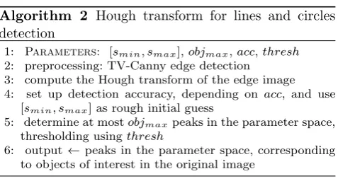
3.1 Pseudocode

Algorithm 2 Hough transform for lines and circles detection

1: _Parameters: [smin, smax],objmax,acc,thresh 2: preprocessing: TV-Canny edge detection

3: compute the Hough transform of the edge image 4: set up detection accuracy, depending on acc, and use

[smin, smax] as rough initial guess

5: determine at mostobjmaxpeaks in the parameter space, thresholding usingthresh

6: output←peaks in the parameter space, corresponding to objects of interest in the original image

4 Method, numerical results, and applications We report in this section the numerical results obtained by the combination of the methods presented for the detection and quantitative measurement of objects in an image.

To avoid confusion, we will distinguish in the follow-ing between two different meanfollow-ings of scale. Namely, by image scale we denote the proportion between the real dimensions (length, width) of objects in the image and their corresponding dimensions quantified in pixel count. Dealing with measurement tools, we talk about measurement scale to intend the ratio between a fixed unit of measure (mmorcm) marked the measurement tool considered and the correspondent number of pixels on the image.

4.1 Male pied flycatcher’s blaze segmentation

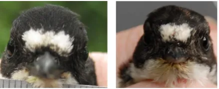
Here we present the numerical results obtained by ap-plying algorithms 1 and 2 to the male pied flycatcher blaze segmentation and measurement problem described in the introduction. Our image database consists of 32 images of individuals from a particular population of flycatchers. Images are 3648×2736 pixels and have been taken by a Canon 350D camera with Canon zoom lens EFD 18–55mm, see Figure 1. In each image one of two types of measurement tool is present: a stan-dard ruler or a surface on which two concentric circles of fixed diameter (1cm the inner one, 3cm the outer one) are drawn. In the following we will refer to these tools as linear and circular ruler, respectively. Here, the measurement scale corresponds to the distance be-tween ruler marks for linear rulers and to the radius of the inner circles for circular rulers.

Figure 1 shows clearly that the scale of the images in the database may vary significantly because of the different positioning of the camera in front of the fly-catcher. In order to study possible correlations between the dimensions (i.e. perimeter, area) of the blaze and significant behavioural factors, the task then is to

seg-ment the blaze and detect automatically the scale of the image considered to provide scale-independent mea-surements.

Parameter choice for Algorithm 1 The GL-segmentation method exploits similarities and differences between pix-els in terms of RGB intensities and texture within their neighbourhood. In our image database these similari-ties and differences are very distinctive and will guide the segmentation step. Recalling Section 2.5, we note that some parameters need to be tuned for the graph GL minimisation. Those are the numberLof Nystr¨om points, the variance σ of the similarity function (2.8), the GL parameterεand the parameterCfor the convex splitting (2.12). However, in our numerical experiments we had to tune these parameters only once. Namely, regarding the choice ofL for both the head and blaze segmentation, we used values not bigger than 5% of the total size of the image considered. The variance appear-ing in the similarity function (2.10) was set toσ2_{= 20} and the weighting parameterε was chosen asε= 0.01 (a smaller choice would create numerical instabilities) and we set the convexity parameter C = 25 or larger in order to guarantee the convexity of the functional appearing in (2.12b).

range are set to 0 (i.e. possible lines or circles within this interval are discarded), while only the ones inside the range (typically, the following line/circle we want to detect) are kept. For our problem, this corresponds to identifying as candidates for ruler notches only the lines away from each other at least smin and at most smax from the peak which has been previously identi-fied. Analogously, the same can be done with circular rulers, where we recall the inner/outer radii are 1 cm and 3 cm, respectively. In this case objmax = 2 since the circular ruler is made of only two concentric circles.

Comparison with Chan-Vese model. Due to the very ir-regular contours and the fine texture on the flycatcher’s forehead, standard variational segmentation methods such as Canny edge detection or Mumford-Shah mod-els, [52, 4, 11, 12], are not suitable for our task, as prelim-inary tests showed. Chan-Vese [19]is not suitable either, mainly because of the small scale detection limits, the dependence on the initial condition, and the parameter sensitivity which may prevent us from an automatic and accurate segmentation of the tiny, yet characteris-tic feathers composing the blaze. In parcharacteris-ticular, the op-timal parametersµ andν appearing in the Chan-Vese functional and a sufficiently accurate initial condition need to be chosen typically by trial and error for every image at hand.

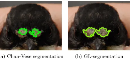
For comparison, we report in Figure 4 the blaze seg-mentation results obtained by using Chan-Vese model (see [19, 20]) and our graph based method which will be described in more detail in the following.

(a) Chan-Vese segmentation (b) GL-segmentation

Fig. 4: Blaze segmentation results computed by using Chan-Vese model [19] and GL minimisation (Algorithm 1). The dependence of the Chan-Vese model on the ini-tial condition and its sensitivity to the model parame-ters may result in inaccurate detections, while the GL approach provides more reliable segmentation results.

4.1.1 Detailed description of the method

We divide our task into different steps:

1. For a given, unsegmented image, we detect the head of the pied flycatcher through a comparison with a user prepared dictionary (see Figure 6) using GL segmentation Algorithm 1. Further computations are restricted to the head only.

2. Starting from the reduced image, a second step sim-ilar to Step 1 is now performed for the segmentation of the blaze, using again Algorithm 1. A dictionary of blazes is used an extended set of features is con-sidered.

3. A refinement step is now performed in order to re-duce the outliers detected in the process of segmen-tation.

4. We use the Hough transform based Algorithm 2 to detect in the image objects witha priori known ge-ometrical shape (lines for linear rulers, circles for circular rulers) for the computation of the measure-ment scale.

5. The final step is the measurement of the values we are interested in (i.e. the perimeter of the blaze, its area and the width and height of the different blaze components). In the case of linear rulers our results are given up to some error (due to the uncertainty in the detection of the measurement scale computed as average between ruler marks distances).

Figure 5 shows a diagram which outlines the work-flow of our method. In order to establish relations with behavioural and biological data confirming or contra-dicting the initial assumption of correlation between blaze size and higher attractiveness presented in the in-troduction [55], we have implemented a user ready pro-gram for the quantitative analysis and measurements of the size of the bird blazes which is currently used by the Department of Zoology of the University of Cam-bridge. The results of this study will be the topic of a forthcoming paper [15].

In the following we give more details about each step.

Step 1: Head detection. We consider unlabelled images in the database and compare each of them with a dic-tionary of previously labelled images, see Figure 6. The training regions (i.e. the heads) are labelled with a value 1, the background with value−1. Unlabelled regions are initialised with value 0.

Photographs of birds with rulers

Hough transf. for detecting orientation of the

ruler

Manually labeled dictionary of bird

heads

Scale detection with Hough transf. perpendicular to

ruler

Graph-based segmentation of bird heads with manually labeled dictionary

Photographs of segmented bird

heads

Manually labeled dictionary of bird

blazes

Graph-based segmentation of bird blazes with manually labeled dictionary

Photographs of segmented bird

blazes Measurement of

bird blazes

Nr

of

p

ix

el

s

Refinement step Possible user input

Fig. 5: The diagram describes the different steps of the segmentation/measurement procedure. Boxes requiring the user input are coloured orange, while the ones where the automatic segmentation/measurement steps are performed are coloured blue. The final objective is coloured green.

Fig. 6: Training dictionary for head detection: the heads are manually selected by the user and separated from the background. Then, the corresponding regions are labelled with 1 while the background is labelled by−1.

will be the number of points needed to produce a sen-sible approximation. We circumvent this issue noticing that at this stage of the algorithm, we only need a rough detection of the head which will be used in the following for the accurate segmentation step. Thus, downscaling the image to a lower resolution (in our practice, reduc-ing the resolution by ten times the original one) allows us to use a small number of Nystr¨om sample points (typically 150–200) to produce an accurate result.

For this first step we use as features simply the RGB intensities and proceed as described in Section 2.5. Once

the head is detected, the resulting image is upscaled again to its original resolution. The solutions computed for the images in Figure 1 are presented in Figure 7.

Fig. 7: Head detection from images in Figure 1 using dictionary in Figure 6

enough to differentiate the blazes from the background consistently in a large number of bird images, due to the colour difference between different blazes. For this step, an additional feature to be considered is the texture of the blaze. For this purpose, we use the MR8 tex-ture featex-tures presented in [67] and proceed as detailed in Section 2.5. For 3×3 neighbourhoods, the feature vector for each pixel will be an element inR99, see Sec-tion 2.5. The Ginzburg-Landau minimisaSec-tion provides the segmentation results shown in Figure 9.

Fig. 8: Training dictionary for blaze segmentation. As in Figure 7 blazes are manually selected by the user and labelled with 1, while black feathers on the background are labelled with−1.

Fig. 9: Blaze segmentation

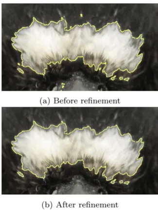
Step 3: Segmentation refinement. This step uses very simple morphological operations in order to remove false detections obtained after Step 2. These can occur due to the choice of colour-texture based features used to com-pute the feature vectors in Step 2. For instance, when looking at Figure 9 (right) we observe that some bits on the left pied flycatcher’s cheek have been detected as they exhibit similar texture properties as the ones on the blaze. In order to prevent this, our software asks the user to confirm whether the segmentation result provided is the expected one or if there are additional unwanted regions detected. If that is the case, using the MATLAB routinebwconncompwe label all the con-nected components segmented in the previous step, dis-carding among them all the ones whose area is smaller

than a fixed percentage (we use 10%) of the largest de-tected component (presumably, the blaze). This works well in practice, see Figure 10. If the user is not satisfied he or she can remove manually the unwanted regions. Figure 11 shows some blaze segmentation results after the refinement step.

(a) Before refinement

(b) After refinement

Fig. 10: Example of segmentation refinement

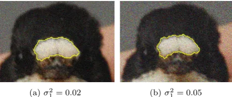
Remark 4 (Robustness to noise)In order to reproduce the more realistic situation of images suffering from noise, we artificially added Gaussian noise with zero mean and different variances to some of the images in our database and performed the three analysis steps of our method. We report in Figure 12 the results corre-sponding to two noise variances (σ2

1= 0.02,σ22= 0.05). The presence of noise influences both the head and blaze segmentation only slightly; the combination of RGB and texture features extracted in the neighbour-hood of each point combined with the comparison to the dictionary make the algorithm robust to noise and allows for an accurate blaze segmentation even in the noisy case.

Fig. 11: Segmentation results after refinement step

(a)σ2

1= 0.02 (b)σ12= 0.05

Fig. 12: Robustness to noise oscillations of GL minimi-sation for binary segmentation. Images have been arti-ficially corrupted with Gaussian noise with zero mean and different variances.

in Section 2.2 and 2.4 for the graph and the opera-tor construction step, respectively, we implemented the MBO segmentation algorithm following [45, Section 2]. We remark that the MBO method has the advantage of eliminating the dependence on the interface parameter ε of the GL functional by means of a combination of heat diffusion and a thresholding step. Instead ofεthe heat diffusion timeτneeds to be chosen. In our numeri-cal implementation we usedτ= 0.005. Since no convex splitting strategies are required in this case, due to the absence of the non-convex double-well term, standard Fourier transform methods are used to solve the re-sulting time-stepping scheme. In Figure 13 we report the blaze segmentation results obtained after applying a refinement step similar to the one described above: we note that a segmentation result comparable to the ones

shown in Figure 11 is obtained. Moreover, robustness to noise is observed also in this case. In terms of compu-tational times, we observed that the replacement of the GL minimisation step with the MBO one did not affect significantly the speed of the segmentation algorithm.

(a) MBO result (b) MBO result,σ2_{= 0.05.}

Fig. 13: Blaze segmentation results obtained by the MBO segmentation algorithm described in [45], after refinement step. Robustness to noise is observed in this case as well. In both numerical tests, the diffusion time is chosen asτ= 0.005.

to detect. In both cases, in order to avoid false detec-tions (such as “aligned” objects erroneously detected as lines, or circle-like objects wrongly considered as circles, see Figure 14), a good candidate for a rough, sensible approximation of the measurement scale is needed as described in Section 3.1. In order to get this, we pro-ceed as follows: after detecting the head as in Step 1, we use the optionEquivDiamof the MATLAB routine regionprops to detect the diameter of the head re-gion (in pixels). We then compare such measurement with pre-collected average measurements of head diam-eters of male pied flycatchers of a similar population (incm), thus obtaining an initial approximation of the measurement scale. In the case of images containing lin-ear rulers, this will serve as a spacing parameter sfor the algorithm. In other words, only lines distant at least spixels from each other will be considered. In the case of circular rulers, the same rough approximation will serve similarly as an indication of the range of values in which the Hough transform based MATLAB function imfindcircles will look for circles’ radii. For linear ruler images, the algorithm will look only for parallel lines aligned with a prescribed direction. We set this direction as the one perpendicular to the longest line in the image (since the expectation is, that this longest line is the edge of the ruler). Results of this step are shown in Figure 15.

Fig. 14: Shadows, blur, noise or other objects in the image may disturb the detection.

Fig. 15: Hough transform used for detecting geometrical objects. Left: lines detection using MATLAB routines houghlines, houghpeaks. Right: circle detection us-ing MATLAB routineimfindcircles.

Outliers removal for linear rulers. The scale detection step described above may miss some lines on the ruler. This can be due to an oversmoothing in the denoising step, to high threshold values for edge detection or also to the choice of a large spacing parameter. Furthermore, as we can see from Figures 1 and 15, we can reasonably assume that the ruler lies on a plane, but its bending can distort some distances between lines. Moreover, few other false line detections can occur (like the number 11 marked on the ruler main body in Figure 15). To ex-clude these cases, we compute the distance (in pixels) between all the consecutive lines detected and eliminate possible outliers using the standard interquartile range (IQR) formula [64] for outliers’ removal. Indicating by Q1 and Q3 the lower quartile and the third quartile, an outlier is every element not contained in the interval [Q1−1.5∗(Q3−Q1), Q3+ 1.5∗(Q3−Q1)]. Finally, we compute the empirical mean, variance and standard deviation (SD) of the values within this range, thus get-ting a final indication of the scale of the ruler together with an indicator of the precision of the method.

Step 5: Measurement. Once the measurement scale has been detected, it is easy to get all the required mea-surements. We are interested in the perimeter, the area of the blaze and also in the height and width of the whole blaze component. For linear rulers, due to the er-ror committed in the scale detection step, these values present some uncertainty and variability (see above). In Table 1 we show the results of numerical tests on a sample of 30 images with linear rulers. For every image in the sample we compute the standard devia-tion (SD) error and report in the table the minimum, maximum, and average SD error over the single ones compute, together with the relative standard deviation (RSD) which gives a percentage indication of the error committed.

RSD:= σ_¯ X ·100,

Uncertainty in the measurements of lengths and ar-eas is calculated with standard formulas in propagation of errors.

Despite these variabilities, our method is a flexible and semi-supervised approach for this type of problem. Further tests on the whole set of images and improve-ments on its accuracy are a matter of future research. The analysis of the resulting data measurements for the particular problem of flycatchers’ blaze segmentation will be the topic of the forthcoming paper [15].

We compare in Table 2 between the use of our com-bined approach and the use of the manualline tool of the IMAGEJ software for the measurement of the blaze area. Namely, we measured in Figure 1b and in Fig-ure 1c the ruler scale by means of the IMAGEJ line tool by considering, for each image, two different 3cm -sections of the ruler; we then measured manually the number of pixels contained in each, divided each mea-surement by 30 and averaged the two results to obtain an estimate of the ruler scale (i.e. the number of pixels crossed by a 1 mm horizontal or vertical line segment). We then measured the area of the blaze after segment-ing it by means of the ‘magic-wand’ [51] IMAGEJ tool and trapezium fitting [55] (see Figure 2). The results are reported in Table 2 both as number of image pixels inside the blaze and in mm2_{, where this second value} has been calculated using the measurement scale de-tected as described above. We then repeated such mea-surements using our fully automated Hough transform method for ruler scale detection, reporting as above the measurements of the blaze area computed both as num-ber of image pixels and inmm2_{. We observe a good level} of accuracy of our combined method (see also Table 1) with respect to the ‘magic-wand’ manual approach of Moreno [51], while, unsurprisingly, the blaze measure-ments obtained by pure trapezium fitting as proposed by Potti and Montalvo in [55] tend to overestimate the area of the blaze.

4.2 Moles monitoring for melanoma diagnosis and staging

In this section we focus on another application of the scale detection Algorithm 2 in the context of melanoma (skin cancer) monitoring, see Figure 3. Early signs of melanoma are sudden changes in existing moles and are encoded in the mnemonic ABCD rule. They are Asymmetry, irregular Borders, variegatedColour and Diameter3. In the following we focus on the D sign.

3 _{Prevention: ABCD’s of Melanoma. American}

Melanoma Foundation, http://www.melanomafoundation. org/prevention/abcd.htm.

Due to their dimensions and their irregular shapes, moles are often very hard to measure. Typically, a com-mon dermatological practice consists in positioning a ruler under the mole and then taking a picture with a professional camera. Sudden changes in the evolution of the mole are then observed by comparison between dif-ferent pictures taken over time. Hence, their quantita-tive measurement may be an indication of a malignant evolution

In the following examples reported in Figure 16, we use the graph segmentation approach described in algo-rithm 1 where texture-characteristic regions are present (see Figure 16a) and the Chan-Vese model [19] for im-ages characterised by homogeneity of the mole and skin regions and the regularity of mole boundaries (Figures (16b)-(16c)). For the numerical implementation, we use the freely available online IPOL Chan-Vese segmenta-tion code [30]. Let us point out here that previous works using variational models for accurate melanoma seg-mentation already exist in literature, see [18, 1], but in those no measurement technique is considered.

4.3 Other applications: animal tracks and archeological finds’ measurement

We conclude this section presenting some other applica-tions for the combined segmentation and scale detection models presented above.

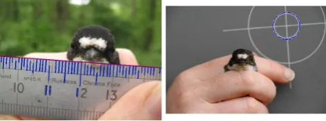
The first application is the identification and classi-fication of animals living in a given area through their soil, snow and mud footprints. Their quantitative mea-surement is also interesting in the study of the age and size a of a particular animal species. As in the prob-lems above, such measurement very often reduces to a very inaccurate measurement performed with a ruler placed next to the footprint image. In Figure 17a4 _our combined method is applied for the measurement of a white-tailed deer footprint.

As a final application, we focus on archaeology. In many archaeological finds, objects need to be measured for comparisons and historical studies [35]. Figure 17b shows the application of our method to coin measure-ments. Due to its circular shape, for this image a com-bined Hough transform method for circle and line de-tection has been used. The example image is taken from [35] where the authors propose a gradient threshold based method combined with a Fourier transform ap-proach. Despite being quite efficient for the particular applications considered, such approach relies in prac-tice on the good experimental setting in which the

SD min SD max mean SD RSD min RSD max mean RSD 4.01 pixels 10.67 pixels 6.81 pixels 6.59 % 17.36 % 11.99 %

Table 1: Precision of the measurement scale detection for linear rulers on a sample of 30 images. The minimum, maximum and average standard deviation (SD) error together with the corresponding relative standard deviation (RSD) errors are reported.

Scale (# pixels = 1mm) Blaze area (pixel count) Blaze area (mm2₎

Manual HT (Ours) MW Trap. GL (Ours) MW Trap. GL (Ours)

Figure 1b 70.2504 72.551 85026 117415 84831 17.2288 23.7917 16.1164 Figure 1c 71.863 71.8367 101730 146751 121360 19.6980 28.4165 23.517

Table 2: Comparison between ruler scale detection by using manual IMAGEJ line tool and our Hough Transform (HT) method with corresponding measurements of the segmented blaze area obtained by using IMAGEJ ‘magic-wand’ (MW) tool [51], trapezium fitting (Trap.) [55] (see also Figure 2) and the graph Ginzburg-Landau (GL) minimisation.

(a) (b) (c)

Fig. 16: Moles’ detection using GL Algorithm 1 (a), the Chan-Vese model [19] ((b),(c)), and measurement scale detection by Hough transform (Algorithm 2).

age is taken: almost noise-free images and very regular objects with sharp boundaries (mainly coins) and ho-mogeneous backgrounds are considered. Furthermore, results are reported only for rulers with vertical orien-tation and no bending.

5 Conclusions

In this paper we consider image segmentation applica-tions involving measurement of a region’s size, which has applications in several disciplines. For example, zo-ologists may be interested in quantitative measurements of some parts of the body of an animal, such as dis-tinctive regions characterised by specific colours and texture, or in animal tracks to differentiate between in-dividuals in the species. In medical applications, quan-tifying an evolving, possibly malignant, mass (like, for instance, skin melanoma) is crucial for an early diag-nosis and treatment. In archaeology, finds need to be measured and classified. In all these applications, often a common measurement tool is juxtaposed to the region of interest and its measurement is simply read directly from the image. This practice is typically inaccurate

and imprecise, due to the conditions in which pictures are taken. There may be noise corrupting the image, the object to be measured may be hard to distinguish, and the measurement tool can be misplaced and far from the object to measure. Moreover, the scale of the image depends on the image itself due to the varying distance from the camera of the ruler and objects to measure.

mea-(a) White-tailed deer tracks measurement (b) Coin measurement, image taken from [35]

Fig. 17: The measurement scale has been detected only in a portion of the figure for the sake of reading clarity.

surements are converted into a unit of measure which is not image-dependent.

Our method represents a systematic and reliable combination of segmentation approaches applied to sev-eral real-world image quantification tasks. The use of dictionaries, moreover, allows for flexibility as, when-ever needed, the training database can be updated. With respect to recent developments [70] in the fields of data mining for the analysis of big data, where predic-tions are often performed using training sets and clus-tering, our approach represents an interesting alterna-tive to standard machine learning (such as k-means) algorithms.

Acknowledgements Many thanks to Colm Caulfield who

has introduced HMR and the bird segmentation problem to us mathematicians and to Andrea Bertozzi for her very useful comments on the manuscript. LC acknowledges support from the UK Engineering and Physical Sciences Research Council (EPSRC) grant EP/H023348/1 for the University of Cam-bridge Centre for Doctoral Training, the CamCam-bridge Centre for Analysis (CCA). CBS acknowledges support from EP-SRC grants Nr. EP/J009539/1 and EP/M00483X/1. More-over, this project has been supported by King Abdullah Uni-versity of Science and Technology (KAUST) Award No. KUK-I1-007-43. HMR is currently supported by an Institute Re-search Fellowship at the Institute of Zoology, by the De-partment of Zoology at the University of Cambridge, and Churchill College, Cambridge.

Appendix A The Nystr¨om extension

With respect to the eigenvalue problem formulation (2.19) and (2.20), we revise in this section the Nystr¨om extension [54] in a matrix form.

Let us define first the sub matricesWXX ∈RL×RL andWXY ∈RL×RS−L as

WXX =

  

w(x1, x1)· · · w(x1, xL) ..

. . .. ... w(xL, x1)· · · w(xL, xL)

 

, (1.21)

WXY =

  

w(x1, y1)· · · w(x1, yS−L) ..

. . .. ... w(xL, y1)· · · w(xL, yS−L)

  .

Analogous definitions hold for WY Y and WY X. Each of these matrices represents the sub matrix having as elements the weights between the points in X, Y or between the two sets. With this notation, the whole matrixW ∈RS×RS can be written in block-form as

W =

WXX WXY WY X WY Y

, WY X =WXYT .

Similarly, vectorsv∈RScan be written asv= (vXT vYT)T. We focus on the spectral decomposition of the first block of W, that is WXX. Since this matrix is sym-metric, calling ΘX the matrix ΘX = diag(θ1, . . . , θL) containining the eigenvalues ofWXX, then by the spec-tral theoremWXX =VXΘXVXT (compare with (2.20)), with VX be the orthogonal matrix having as columns the eigenvectors ofWXX. Writing (2.19) fory ∈Y, in operator form, we obtainVY as

VY =WY XVXΘX−1.

The approximated eigenvectors ofW can then be writ-ten in matrix form as

V =

VX WY XVXΘX−1

. (1.22)

Let us observe that

V ΘXVT =

VX WY XVXΘ−X1

ΘX [VXT (WY XVXΘX−1) T_]

=

VXΘXVXT WXY WY X WY XWXX−1WXY

(1.23)

=

WXX WXY WY X WY XWXX−1WXY

Therefore, Nystr¨om extension can be interpreted as the approximation W ≈ V ΘXVT, under the approxima-tion of WY Y given by WY Y ≈ WY XW_XX−1WXY. The quality of the approximation of the full W is quanti-fied by the norm of the Schur complement kWY Y − WY XW_XX−1WXYk, see [28]

Recalling the definition of the symmetric graph Lapla-cian Ls given by (2.8) and the relation between the spectral decomposition ofW and the one ofWin (2.16), we observe that a normalisation step now needs to be computed for obtaining the spectral decomposition of Ls. Defining1Las theL-dimensional vector consisting of ones and 1S−L analogously, we use (1.23) and start computing the nonnegative vectord= (dT_XdT_Y)T by

dX dY =

WXX WXY WY X WY XWXX−1WXY

1L 1S−L

(1.24)

=

WXX1L+WXY1S−L WY X1L+WY XWXX−1WXY1S−L

.

Therefore, the matrices WXX and WXY can be nor-malised simply by considering:

ˆ

WXX =WXX./(

p

dX⊗

p

dX T

), (1.25)

ˆ

WXY =WXY./(

p

dY ⊗

p

dY T

),

where the division is intended element-wise and ⊗ is the standard vector tensor product.

A further step of normalisation is now needed since the approximated eigenvectors of W, i.e. the columns of the matrixV in (1.22) may not be orthogonal. Such normalisation may be obtained by using auxiliary uni-tary matrices. We refer the reader to [10, Section 3.2] for more details on this.

Once these additional normalisation steps are com-pleted, we then get a spectral decomposition of W in terms of its eigenvalues ˆλi and the corresponding nor-malised eigenvectorsvi, i= 1, . . . , S. Therefore, recall-ing (2.16), the spectral decomposition ofLsis given in terms of the eigenvalue 1−ˆλi and eigenvectorsvi.

Appendix B The MBO scheme for image segmentation

As previously commented in Section 2.1, by taking the L2_{gradient descent of the Ginzburg-Landau functional} defined in (2.1), one gets the well-known Allen-Cahn equation [3]:

ut=ε∆u− 1 εW

0_{(u), (2.26)}

which has often been studied for the modelling of sev-eral phase transition and separation problems and for

the study of mean curvature flow (see, e.g., [13]). In the limit → 0 solutions consist of two phases corre-sponding to the wells ofW. In [57] it is shown that, for rescaled solutions of equation (2.26), the interface be-tween these phases evolves according to mean curvature flow. In [47], Merriman, Bence and Osher propose an al-ternative approach (later named MBO scheme) which, by using threshold dynamics, approximates the mean curvature flow of the interface at discrete times. As proved rigorously in [6], for small values of the inter-face parameterε, the MBO scheme can then be used to solve equation (2.26) numerically.

In [45], the authors propose a variant of the MBO scheme as an alternative way to (approximately) min-imise the graph GL functional with fidelity term, (2.9). Recalling the graph framework introduced in Section 2.2, the MBO segmentation starts from an initialisa-tionU1 given by (2.14) and computes, for everyn≥1 the new iterateUn+1 fromUn by applying sequentially the two following steps:

– Step 1(diffusion with forcing term): Starting from U_n1=Un, solve for every 1≤k≤K the discretised heat diffusion equation with fidelity term

Uk+1 n −Unk

τ =−LsU k+1

n −χ(x)(U k+1

n −U0), (2.27)

where τ := ∆t_K is the heat diffusion time and K is the number of diffusion steps. Practically, τ has to be chosen small enough to approximate the mo-tion by mean curvature and large enough to avoid freezing orpinning, which occurs when the diffusion time is so short that not enough mass diffuses along the edges of the network and the thresholding op-eration described in the following Step 2 leaves Un unchanged.

– Step 2(thresholding): For every point x setUn+1 as:

Un+1(x) =

(

1, ifUK

n (x)≥0, −1, ifUnK(x)<0.

Numerically, (2.27) is solved at each diffusion time step kτ, k ≥ 1 by considering the spectral decomposition of Uk

n with respect of the eigenvectors of the operator Ls, similarly as in (2.15), and using classical Fourier transform methods to compute the new iterateUk+1

n .

Appendix C The Hough transform