A comparison of gridded sea surface temperature datasets for marine ecosystem studies

INTRODUCTION

The study of the effects of ocean variability on mar-ine ecosystem structure and functioning requires clear indicators of the changing physical habitat. Spatial and temporal variations in oceanographic conditions have significant influences on ecological processes and how biological resources are dis -tributed (Lutjeharms et al. 1985, Pollard et al. 2002). Thus, for example, variation in temperature and sa li -nity, as well as structural features such as currents, all can correlate well with primary production (Pol-lard et al. 2002), and even higher trophic levels might

be influenced to a varying extent by the physical properties of the water column (Charrassin & Bost 2001). Nonetheless, clear relationships are not ne -cessarily apparent; for example, because of dilution effects and temporal and/or spatial lags in ecological response (e.g. Guinet et al. 2001, Bradshaw et al. 2004, Todd et al. 2008).

Linking oceanographic conditions to changes in the marine ecosystem is challenging, because tradi-tionally these are described at different scales, both in space and time (Brown et al. 2011). Oceanographic in situ data typically derive from line transects or mooring observations, both of which are temporally

© The authors 2014. Open Access under Creative Commons by Attribution Licence. Use, distribution and reproduction are un -restricted. Authors and original publication must be credited. Publisher: Inter-Research · www.int-res.com

*Corresponding author: [email protected]

Comparison of gridded sea surface temperature

datasets for marine ecosystem studies

Lars Boehme

*, Mike Lonergan

_{, Christopher D. Todd}

1_{Scottish Oceans Institute, University of St Andrews, St Andrews KY16 8LB, UK} 2_{Present address : University of Dundee, Dundee DD1 9SY, UK}

ABSTRACT: In assessing impacts of a changing environment on the structure and functioning of marine ecosystems, the challenge remains to distinguish the effects of noise and of temporal and spatial autocorrelation from environmental drivers of biotic change. One analytical approach is to de-trend the data and use the resulting residuals; an alternative method involves use of the raw anomalies and a reduction of the degrees of freedom (df )to make the hypothesis testing more conservative. Here, we assess the comparability of 3 gridded sea surface temperature (SST) datasets — ERSST V3b, HadISST, and OISST V2 — to in situ measurements. The 1° gridded HadISST and OISST V2 showed the highest similarity, while the weaker correlations with ERSST V3b probably are attributable to its coarser 2° grid. We investigated the performance of 2 com-monly applied statistical methods to resolving autocorrelation, and proceeded to correlation analyses between the SST datasets and 2 contemporaneous 15 yr time-series of the somatic growth condition of annual cohorts of Atlantic salmon Salmo salar, which migrate to the Norwe-gian Sea. For these latter analyses, reducing dfcould not fully resolve the problem of high positive autocorrelation. The 3 oceanographic datasets do not provide the same correlative outcomes and levels of significance with the salmon time-series. When analysing time-series that pre-date the availability of satellite data, the choice of dataset is restricted to either ERSST V3b or HadISST; but for recent studies (1982 onwards) OISST V2 also is available, and it will be important to assess the relative merits of the 3 SST data sources when interpreting contrasting correlative outcomes.

KEY WORDS: Oceanography · Time-series · Autocorrelation · Sea surface temperature · Salmon

O

PEN

PEN

and spatially very restricted. Such data are therefore seldom used by biological oceanographers, except when biological data (e.g. from acoustic surveys, towed nets, bottle samples) are collected simultane-ously (e.g. Ward et al. 2002). To overcome these limi-tations, data from the Argo global array of profiling floats can be used. These drifting floats deliver verti-cal temperature and salinity profiles to depths up to 2000 m and are distributed throughout the World Ocean at an average 3° spacing (Gould et al. 2004). These devices now are equipped with fluorescence or dissolved oxygen sensors which provide informa-tion about condiinforma-tions relevant to the base of the food web (Xing et al. 2012). The Argo monitoring system is, however, of limited coverage at high latitude, because the floats require ice-free waters to surface and transmit their data. Despite this constraint, and whilst the spatial and temporal resolution of the Argo array remains coarse compared to the typical ‘patch-iness’ of marine ecosystems, it does continue to provide tractable, broad-scale data of value both to phy sical and biological oceanographers.

More recently, the ability to track movements and behaviour of individual top predators, whilst simulta-neously gathering linked ocean observations, has been possible with animal-borne instruments (Boehme et al. 2009). Because both datasets are recorded on the same scale, these devices enable the assessment of linkages between behavioural chan -ges and the immediate physical environment of the instrument-carrying animal (Bailleul et al. 2007, Biuw et al. 2007). It must, however, be acknowledged that one limitation is the size of these instruments and the consequential restriction of their deployment only on large, high trophic level consumers.

Sea surface temperature (SST) has been measured by satellites for several decades, with a standard deviation of 0.1 to 0.5°C and a spatial resolution between 1 and 50 km (McClain et al. 1985, Reynolds et al. 2005), but data acquisition often is hampered by cloud cover.

These examples illustrate that commonly there either are mismatches in scale between datasets de -scribing the physical marine environment and eco-system, or that derived information may be restricted in relevance either to the lowest (indirect) or highest (direct) trophic levels. To obtain long time-series with high temporal and spatial resolution of directly meas-ured ocean properties, especially for geographically remote or inaccessible locations, behavioural studies generally have relied on optimal interpolated grid-ded fields of remotely-sensed satellite data of, for example, SST and sea level anomaly (Bradshaw et al.

2004, Todd et al. 2008, Jensen et al. 2011). One major advantage of these data sources lies in their allowing a synoptic overview of changing features over large areas. Some of these fields are based on a combina-tion of satellite and in situobservations and provide improved spatial coverage in comparison to the lim-ited sets of long in situtime-series. Although the tem-poral resolution of remotely acquired data can be very high (e.g. daily), the spatial resolution can be compromised by interpolation in the processing of sparse data (see also Reynolds & Chelton 2010). Routinely available SST fields generally are produced with a view to representing long-term trends and variability on spatial scales ranging from the ocean basin to global, and with the aim of improving long-term climate records (Reynolds et al. 2002). In a comparative assessment of different empirical data sources, Hughes et al. (2009) analysed gridded SST data together with associated time-series of in situ measurements and noted that different SST fields can diverge by up to 1°C. Moreover, they showed that the timing of extreme events can differ from that indicated by in situmeasurements. Notwithstanding those contrasts, a further impediment of these data -sets — which may be critical to biological oceano-graphic studies — is that these SST fields describe only ocean surface conditions, which might not rep-resent the correct habitat (Sims et al. 2001, 2004).

resulting residuals, whilst the alternative involves a reduction of the de grees of freedom (df ) applied in correlation analyses (Pyper & Peterman 1998).

Here, we investigate 2 statistical methods to assess the linkage be tween SST and the mean somatic growth condition of annual cohorts of adult At -lantic salmon Salmo salar (hereafter salmon). Salmon are op por tunistic, generalist predators of zooplankton and nekton and their foraging probably is predominantly confined to the top 10 m of the water column (Jacobsen & Hansen 2000, Rikardsen & Dempson 2011). SST anomalies (de rived from the OISST V2 satellite dataset) in the salmon foraging area of the Norwegian Sea exert indirect effects on cohort growth success by influencing the quality and quantity of available prey (Todd et al. 2008). A weak-ness of the analysis was their utilization only of the OISST V2 dataset; here we assess the comparability of the 3 publicly available gridded SST data sources. We investigate how well these fields compare to in situ measurements by focusing on temperature anomalies both on seasonal and shorter time scales. We then investigate how the changes in SST fields correlate with 2 independent but contemporaneous time-series of changes in salmon population condi-tion factor by applying the 2 distinct statistical meth-ods in resolving the problem of autocorrelation.

MATERIALS AND METHODS Gridded sea surface temperature datasets

In recent years a number of extended historical observed temperature analyses have been produced for use in climate studies. Here, we focus on 3 glob-ally gridded SST datasets (Table 1, Fig. 1) and con-fine the analysis to the period 1950 to 2010, when behavioural studies and biological time-series be -came more common.

The NOAA Extended Reconstructed Sea Sur -face Temperature (ERSST V3b) dataset is derived from the International Comprehensive Ocean-Atmosphere Data Set (ICOADS)

(Smith et al. 2008, Woodruff et al. 2011). This source comprises in situ observations from many dif-ferent measurement technologies, and is statistically processed to allow for sparse data in creating the gridded field (Smith et al. 2008). Satellite SST data also were integrated in a previous version,

but this introduced a small residual bias to wards colder temperatures and their inclusion was discon-tinued. Surface sea ice concentrations (i.e. percent cover) be tween 60 and 90% are used to force the analysed SST linearly towards the freezing point of seawater (−1.8°C), with all grid cells of > 90% ice cover set to that freezing point; this can be important locally in the marginal-ice zones (Smith et al. 2008). The Hadley Centre Sea Ice and Sea Surface Tem-perature (HadISST) fields are based on in situ ob -servations and satellite-derived estimates from 1870 to present. In situ data from the Met Office Marine Data Bank (MDB) — including observations compiled since 1982 through the Global Telecommunication System (GTS) and monthly satellite SST data from January 1982 on wards — have been analysed using a Reduced Space Optimal Interpolation technique (Rayner et al. 2003). At times, and in areas, with sparse data coverage, monthly median SST data for 1871 to 1995 from ICOADS also were used in cases of a lack of available MDB data. SST near sea ice is esti-mated using statistical relationships be tween SST and sea ice concentration. Rayner et al. (2003) state that ‘SSTs near sea ice can be several degrees higher than freezing when there is high insolation and light winds’. They therefore chose to apply a quadratic relationship between sea ice concentration and SST in preference to a linear fit. These quadratic relation-ships were de termined by inspection of scatterplots for each grid cell and based on 3 mo, centred on the target month.

NOAA’s Optimum Interpolation (OI) Sea Surface Temperature (SST) data set (OISST V2) is based on in situdata received through the GTS and satellite-derived SST (Reynolds 1988), and comprises weekly fields dating back to December 1981 (Fig. 1, Table 1). As for HadISST, SST near sea ice is estimated using a quadratic relationship, which in turn is calculated separately for each longitudinal sector in each hemi-sphere and calendar month (Reynolds et al. 2002). Monthly fields are derived by a linear interpolation of the weekly fields to daily fields and then by averag-ing the daily values over 1 mo.

Name Start date Resolution Data sources

Space Time

NOAA ERSST V3b 01/1854 2°×2° monthly in situ

Hadley Centre HadISST 01/1870 1°×1° monthly in situ, satellite NOAA OISST V2 12/1981 1°×1° monthly in situ, satellite Table 1. Key features of gridded sea surface temperature (SST) datasets used in

Fig. 1. Gridded sea surface temperature (SST) fields used to estimate the mean monthly eastern North Atlantic SST and SST anomaly for ERSST V3b, HadISST and OISST V2 datasets (example month shown, July 2008). The position of OWS Mike (66° N, 2° E) is indicated by a black dot. The ranges for the 2 kernels (σ= 250 and 500 km) are indicated by green circles.

In addition to the monthly SST fields, monthly cli-matologies and monthly anomalies also are available. A climatology represents the mean value for a grid cell over an extended time period (usually 30 yr), whereas an anomaly is the deviation from that mean. However, these climatological datasets are not based on the same time period. NOAA provides a monthly, long-term (1971−2000) mean climatology for ERSST V3b, and 2 datasets of monthly anomalies are available for OISST V2. The latter are based on climato -logies using both in situobservations and OISST V2 data for the periods 1961 to 1990 and 1971 to 2000

(Reynolds & Smith 1995, Xue et al. 2003). The Hadley Centre provides neither a climatology nor monthly anomalies for the HadISST data set. For present purposes we therefore calculated a monthly climatology for each grid cell based on the 1971 to 2000 HadISST data. Thus, we have contemporaneous climatologies and these were used to calculate monthly SST anomalies for each SST field (Figs. 1 & 2).

In situSST data

Ocean Weather Ship Station (OWS) Mike (66° N, 2° E) is operated by the Norwegian Meteorological Institute and has provided the longest homoge-neous time-series from the deep ocean (2200 m) in the eastern margin of the Norwegian Sea deep basin (Gammel-srod et al. 1992). Temperature and salinity profiles have been collected daily to 1000 m, and weekly to 2200 m, since 1 October 1948 (www. eurosites. info/stationm.php). Here, we focus on the nearly uninterrupted ocean tem-perature time-series for the upper 10 m. To obtain a temporally continu-ous surface time-series, we used the surface measurements wherever pos-sible. If they were not available we took the next available measurement down to a maximum depth of 10 m. If more than one measurement was available per day, we took the mean value. As a rule, this provides SST estimates on alternate days. For every month with >10 daily measurements, a mean was taken. The monthly variability (SD) was on average ± 0.5°C, but on occasion exceeded ±1°C. Monthly values from January 1971 to December 2000 inclusive were used to calculate a monthly climato -logy, which in turn was used to calculate monthly SST anomalies for the whole time-series (Fig. 2).

Salmon condition factor

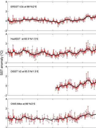
Data for return migrant adult 1 sea-winter (1SW) salmon were sampled repeatedly throughout each Fig. 2. Monthly sea surface temperature (SST) anomalies (grey dots) for the

annotated grid point, derived from a 1971−2000 climatology, for 3 gridded datasets and OWS Mike. The fitted trend line (black) is a weighted running mean with a Gaussian window of σ= 1 yr. Residuals between the trend line

summer netting season (June–August) at Strathy Point (SP), North Scotland (58° 36’ N, 4° 00’ W) and in the River North Esk (RNE) estuary, East Scotland (56° 46’ N, 2° 26’ W) (Todd et al. 2008). SP comprises ‘mixed stock’ data for fish originating from multiple (unknown) river populations, whilst RNE data per-tain to that specific river stock. For the present study, we used data collected between 1993 and 2007 inclu-sive, which includes an additional final year of data (up to closure of the SP fishery in 2007) compared to those presented by Todd et al. (2008). Annual sample totals at SP ranged from 115 (1999) to 689 (1996) fish, with a median of 384. Catch data from RNE are com-mercial-in-confidence, but sample sizes were large and typically exceeded those from SP, with the ex -ception of 1995 (434 fish). Todd et al. (2008) computed condition factor as the predicted weight (PWt) of fish at a standard length (60 cm, SP; 58 cm, RNE). Here, we express condition factor as the annual mean Rel-ative Mass Index (Wr; Blackwell et al. 2000; see Todd et al. 2008 for details). PWt and mean Wrare highly correlated (SP: r = 0.998, n = 14, p < 0.001; RNE: r = 0.997, n = 14, p < 0.001) and the time-series for PWt (Todd et al. 2008) and Wr (Fig. 4) for either sets of salmon data showed an identical pattern of residuals. Previously, Todd et al. (2008) analysed spatial ker-nels of SST variation centred at 67.5° N, 4.5° E, which was the assumed centre of distribution of Scottish salmon exploiting the Norwegian Sea. Because of the constraint of the fixed position of OWS Mike (at 66° N, 2° E) the kernels utilised in the present com-parative study are further south and east of those of the previous study. This had no effect on the de -tection of significant results for SP salmon and the comparable analyses of residuals for OISST V2.

Autocorrelation

All the present time-series show progressive change, with a high degree of positive autocorrela-tion. This presents a major statistical and analytical challenge in not conforming to the assumption of serial independence of the data. One approach to resolving this problem is to remove autocorrelation by predicting a sample based on information from each of the time-series. The difference between the predicted value and the sample value (residual) for a given time-series will be less related to the remain-der of the sample values (‘pre-whitening’). In the case of the SST fields, the first step is to apply the cli-matology for each dataset to generate monthly SST anomaly fields (Fig. 1). This ensures a de-seasoned,

monthly anomaly time-series for each grid point. The data then are de-trended by applying a high-pass filter using a Gaussian-weighted running mean (σ= 1 yr). Finally the residuals between the smoothed time-series and the SST anomalies are calculated (Fig. 2). This is undertaken for each grid point of the 3 SST fields, but more regional estimates were calcu-lated here by using a spatially weighted analysis; spatial kernel widths of σ= 250 and 500 km (centred on 66° N, 2° E for each gridded data set) were gen -erated monthly with data weightings, which were defined using Gaussian kernels, assigned to each SST anomaly grid point according to its distance from the central reference grid point (Fig. 1). These 2 ker-nel sizes provided time-series that are independent of the resolution and grid cell centres of the different gridded fields and thereby permitted assessment of spatial scale on the correlations. As before, these time-series then were de-trended by application of a Gaussian-weighted running mean (σ= 1 yr) and the residuals calculated.

The first step is omitted for the annual salmon con-dition factor time-series, which was de-trended using only a Gaussian-weighted running mean (σ= 1 yr). The resulting time-series are essentially free of auto-correlation and classical hypothesis testing is appro-priate. However, as a consequence of the extensive preliminary filtering of data, statistical power of the final correlation analyses might be expected to be redu ced using this technique.

The second approach is to not filter the data, but rather to increase the stringency of the hypothesis testing procedure by applying fewer df for correla-tion analyses. Here, we follow Pyper & Peterman (1998) and utilize their Eqs. 1, 6 & 7 according to their recommendations for short time-series (hereafter the Pyper & Peterman method, PP). The ‘effective’ (= ad -justed) degrees of freedom (df*) then are given as:

(1)

The autocorrelation rXXof the time-series X is esti-mated over the first df/5 lags (j = 1 to df/5) using the Modified Chelton method, as described by Pyper & Peterman (1998), and the estimator recommended by Box et al. (2008):

(2)

This technique depends on being able to identify the autocorrelation functions, which can be only

1 2

1 2

1 5

df df df rXX j r j

j df

YY

*+

(

)

∑

( )

( )

r j df

df j

X X X X

XX

t t j

poorly estimated for short time-series: in such cases, statistical power might be reduced and Type 2 errors thereby increase. For short time-series the resulting df* can be greater than dfand in such cases we con-strained df* to be no greater than df(Pyper & Peter-man 1998).

RESULTS

Comparison of time-series at OWS Mike In order to draw comparisons amongst the 3 grid-ded SST datasets, and to assess them against in situ measurements, data from the single grid point closest to the OWS Mike position at 66° N, 2° E were extrac -ted from each dataset (Fig. 2). All time-series show the same trend pattern, and extreme events (e.g. the cold event in 1989) were captured by the residuals in all data sets.

ERSST V3b shows a dampened curve when com-pared to the other time-series. The residuals also are generally smaller, SD ± 0.26. This is expected be -cause of the 2° grid, which averages in situdata over a greater spatial extent than do the other data sets. HadISST shows more features and SD ± 0.42 for the converse reason. Nonetheless, the timing of extreme points in the curves was very similar, with better con-formation since the mid-1980s, when more detailed

in situoceanographic data became available. Prior to that time, the curves show some differences because the gridded field relies more on its interpolation scheme than on the limited assimilated data. The short OISST V2 time-series shows high variability both for SST anomaly and also for the residuals (± 0.44 SD). HadISST and OISST V2 (Fig. 2) show similar trends because the OISST V2 data (when available) are incorporated into the HadISST fields. The in situ data from OWS Mike show the highest variability for the residuals (SD ± 0.46) and, as ex -pected, the occurrences of warm or cold events typi-cally were of briefer duration than for the gridded time-series. Again, this is attributable to OWS Mike data not being spatially averaged, and extreme events move past the fixed position more quickly than through a 1° or 2° grid cell.

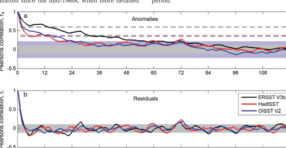
Fig. 3 shows the autocorrelation sequences for the SST anomalies and residuals, normalized so that the values at zero lag are identical (r = 1). These data include all 3 time-series, and are based on their common 29 yr period (1982−2010) and pertain to the same grid cells illustrated in Fig. 2. ERSST V3b showed the highest autocorrelation, which again is attributable to its coarser spatial scale. As before, HadISST and OISST V2 provide very similar results, largely because both datasets include the satellite measurements over this time period.

Fig. 3. Normalized autocorrelation sequences for (a) sea surface temperature (SST) anomalies and (b) residuals taken from the 3 time-series in Fig. 2. The shaded boxes show intervals of r ± 0.11 (grey) and ± 0.22 (blue). The dashed lines in the top panel show the critical values (α = 0.05) based on Pyper & Peterman (1998) for the ERSST V3b (black), HadISST (red) and OISST V2

The standard critical value of r (2-tailed) at a signif-icance level of α = 0.05 and n = 348 observations was ~0.11. The 3 SST anomaly time-series do retain sig-nificant autocorrelation: however, such a long de-correlation scale reflects that although the climato-logical mean values were removed, a systematic change in the mean values remains observable and the time-series were not stationary. It is necessary, therefore, to increase the stringency of the test be cause some of the consecutive observations still re -main strongly correlated. One possibility is to re duce the α-value to account for the number of comparisons (N) being performed. The simplest and most conser-vative approach is the Bonferroni correction (Miller 1981), which sets the α-value for each comparison to αb= α /N, resulting in αb= 0.000144 and a critical value for r of ~0.22. Even so, the results show signifi-cant outcomes for lags up to 2 yr for HadISST and OISST V2, and > 4 yr for ERSST V3b. Accordingly, this simple analytical approach remains highly af fec -ted by the long-term trends seen in Fig. 2. Moreover, all results show some evidence of a sinusoidal sea-sonal cycle (Fig. 3b).

The de-trended residuals (Fig. 3b) show no indica-tion of significant autocorrelaindica-tion be yond a lag of 3 mo, which conforms to the mesoscale time scales expected. Longer time lags do not satisfy Bonferroni correction and are not significant, so the pre-whiten-ing method delivers plausible results. Of interest, however, are the maxima both for the anomalies and residuals detectable at approx. 6 yr. This positive autocorrelation could be the result of a set of har-monic and sub-harhar-monic temperature cycles intro-duced by the Earth’s nutation of 18.6 yr. For example, a similar temperature cycle of 18.6/3 = 6.2 yr has been demonstrated in the Barents Sea (Yndestad 1999), and this effect has an impact on water-mass variations (e.g. Osafune & Yasuda 2012).

The alternative approach in accounting for auto-correlation (the PP method and adjustment of df ) requires recalculation of the significance levels applicable to each time-series (Fig. 3a). ERSST V3b showed the highest autocorrelation and accordingly the adjusted df were reduced to df*E = 10, with the critical value for rraised to 0.58. The dffor OISST V2 were adjusted downwards to df_O*= 27 (critical value of 0.37), whereas HadISST showed the lowest auto-correlation and the adjustment was only reduced to df*_H= 32 (critical value 0.34). Using these time series-specific significance levels, only observations within ca. 15 mo of one another showed significant correla-tion (Fig. 3a). This is significantly longer compared to that for the residual method.

Both methods can be used to investigate long SST time-series, and can resolve the problem of high pos-itive autocorrelation within the time-series. Pre-whitening does, however, result in loss of information because of its conservatism by the removal of the low frequency variability and in being based on a fixed significance level, whilst the PP method is focused on the individual anomaly time-series and estimates a longer (and perhaps more meaningful) de-correla-tion scale. Accordingly, we then proceeded to further assess these 2 methods by comparing amongst the 3 time-series. We used the time-series based on spa-tially-averaged 250 and 500 km Gaussian kernels

Kernel HadISST OISST V2 OWS

250 km

ERSST V3b r 0.814 0.822 0.711

rcrit 0.480 0.532 0.399

N 15 12 23

HadISST r 0.931 0.865

rcrit 0.411 0.327

N 21 34

OISST V2 r 0.884

rcrit 0.360

N 28

500 km

ERSST V3b r 0.814 0.833 0.703

rcrit 0.542 0.613 0.426

N 11 9 20

HadISST r 0.941 0.834

rcrit 0.461 0.335

N 17 33

OISST V2 r 0.851

rcrit 0.380

N 25

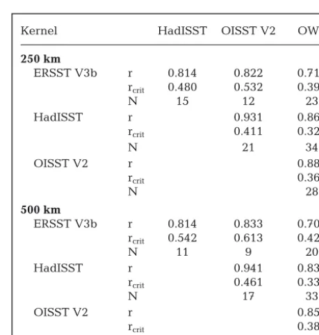
Table 2. Pearson correlation coefficients (r) between differ-ent SST anomalies in the North Atlantic (Fig. 1). Coefficidiffer-ents are based on 2 Gaussian kernels with 250 and 500 km radius

and the in situtime-series at OWS Mike

Kernel HadISST OISST V2 OWS

250 km

ERSST V3b 0.668 0.603 0.548

HadISST 0.872 0.789

OISST V2 0.828

500 km

ERSST V3b 0.661 0.582 0.522

HadISST 0.893 0.735

OISST V2 0.769

centred on the OWS Mike position (66° N, 25° E). These time-series were cross-correlated and we assessed the significance patterns in the residuals (pre-whitening) versus the anomalies based on the PP method.

As expected, all the time-series were highly cross-correlated and all results were significant, because they represent the same SST both in time and space. HadISST and OISST V2 showed the highest correla-tions both for anomalies (Table 2) and residuals (Table 3), owing to their shared satellite data. The weaker correlations for ERSST V3b are attributable to its coarser grid and consequential inability to resolve mesoscale oceanographic features. These differing data sources will not necessarily show closely comparable results when correlated against biological or ecological time-series data. Choice of SST database can therefore have important qualita-tive and quantitaqualita-tive consequences for the outcomes of targeted biological analyses (see also Reynolds & Chelton 2010).

Effect of SST on salmon condition

In light of the contrasting results in Tables 2 & 3, we here extend the previous analysis of Todd et al. (2008) for the 2 salmon time-series to include comparisons with ERSST V3b and HadISST, and apply also the PP method. Fig. 4 shows the close conformity between the 2 independent salmon time-series, and the gen-eral decline in condition factor as SST anomalies rose. The correlation coefficients between the raw values of salmon condition and OISST V2 anomalies were consistently negative, with the strongest corre-lations at a time lag of −2 yr (Table 4); that is, 1 yr before the salmon cohorts migrated to sea. Analyses between de-trended residuals of sal mon condition factor and SST anomalies show similarity of pattern, and OISST V2 and HadISST (which share satellite data during the period analysed) delivered closely similar results (Figs. 5 & 6); but, importantly, there are some clear differences to ERSST V3b, especially for the SP sal mon time-series (Fig. 6).

River North Esk (RNE) salmon time-series

The results herein for the 15 lagged months’ correlations between the re -siduals of RNE salmon condition factor and SST anomaly for OISST V2 (Fig. 5) are almost identical to those presented

Fig. 4. Raw values (dots) and smoothed time-series (solid lines) of annual mean condition factor for adult 1 sea-winter Atlantic salmon Salmo salarcaptured at the River North Esk (black) and Strathy Point (blue), Scotland. Weighted running means (σ= 1 yr) were used to de-trend these data and to generate residuals (red) for lagged correlation analysis. For visual comparison with the salmon time-series, the mean smoothed monthly sea surface temperature (SST) anomalies from OISST V2 are shown in grey

Time lag of July SST (yr)

0 −1 −2 −3 −4 −5 −6

River North Esk −0.464 −0.697 −0.718 −0.595 −0.356 −0.085 0.058 Strathy Point −0.402 −0.550 −0.754 −0.550 −0.326 −0.267 0.034 Table 4. Pearson correlation coefficients between raw condition factor for Atlantic salmon Salmo salar from Scotland (1993−2007), and raw monthly

by Todd et al. (2008). Minor differences are attributa-ble to the additional year of data included in the pres-ent analysis, and the differpres-ent location of the kernels utilised. The inclusion of the year 2007 provides not only an extra empirical annual value, but also influ-ences the fitted smooth curve (and hence the residu-als) in the final years of the time-series. The analysis

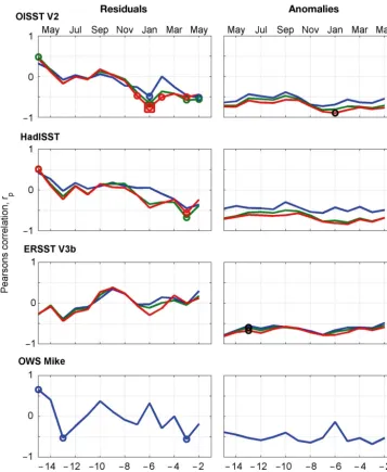
assessed monthly lags from −2 mo (May of the year of capture) to −15 mo (April of the previous year, when the juvenile smolt cohorts will have commenced emigration to sea). As a comparison with the gridded data -sets, the correlations with OWS Mike are shown also. There were strong negative correlations at −2 mo (May) and −5 mo (February), and positive results Fig. 5. Left panels: Correlation analyses between residuals for the Atlantic salmon Salmo salarcondition factor time-series (1993−2007) for the River North Esk, Scotland, and sea surface temperature (SST) residuals from mean monthly SST anomalies (lag in months on x-axis) extracted from the 3 gridded datasets and the in situtime-series at OWS Mike. Significant correla-tions (α= 0.05) are denoted by a circle, and results satisfying Bonferroni correction are denoted by a square. Right panels: Analyses between salmon condition factor time-series and monthly SST raw anomalies. Significant outcomes for df* according to the Pyper & Peterman (1998) method are denoted by a circle (but note that the one significant result did not pass Bonferroni correction for multiple tests). The analyses included grid point data (blue) and weighted Gaussian kernels of 250 km

at −9 mo (October) and −10 mo (September). For HadISST, the correlations at the shorter time lags were weaker. Whilst some results satisfied the standard significance level, none passed Bonferroni correction (αb = 0.0036). ERSST V3b conformed to OISST V2 and HadSST in showing positive correla-tions, but differed in indicating these at shorter time lags. The only correlation satisfying Bonferroni cor-rection was the positive ERSST V3b result for Octo-ber. Results for the in situOWS Mike time-series fol-lowed the same general pattern as HadISST and OISST V2, but none were significant.

The patterns of correlation between RNE salmon condition factor and the SST anomaly time-series

were negative for all time lags, and with only minor differences apparent for the 3 gridded data sources. Only 1 correlation at −11 mo for OWS Mike was significant following correction for autocorrelation using the PP method, but that result did not pass Bon-ferroni correction for multiple tests.

−6 mo (January) for OISST V2 anomalies was signifi-cant, but did not satisfy Bonferroni correction. By contrast, ERSST V3b anomalies showed no sig ni -ficant winter results, but a negative correlation at −13 mo (June of the year of river emigration). No significant results were detected for OWS Mike.

The results of the 15 correlations between the re -siduals of SP salmon condition factor and OISST V2 residuals (Fig. 6) are almost identical to the results presented by Todd et al. (2008) for 1993 to 2006. Strong negative correlations at short time lags (<−8 mo) are apparent for OISST V2, HadISST and OWS Mike, but the only result to satisfy Bonferroni correction (αb = 0.0036) was that for OISST V2 at −6 mo (January), as reported by Todd et al. (2008) — albeit for a kernel focus of 67.5° N, 4.5° E. The 2 HadISST kernels showed a qualitatively similar pat-tern, but no results passed Bonferroni correction (αb= 0.0036), and OWS Mike showed no significant results. The particularly striking outcome for SP is that whilst OISST V2 and HadISST did provide some significant outcomes, ERSST V3b showed no signifi-cant results.

With respect to the application of the PP method as an approach to resolving the analytical problem of autocorrelation, we did, in some instances (< 2%), find the estimate of the effective degrees of freedom (df*) to exceed the number of observations. This can arise from variability in the estimates of autocorrela-tion amongst the separate lag calculaautocorrela-tions and, as recommended by Pyper & Peterman (1998), in these cases we constrained df* to a maximum of N. This occurred only for correlations between the salmon and OISST V2 and HadISST time-series at a lag of –10 mo, indicating a high degree of variability in the autocorrelation estimates from these 2 SST ano -maly time-series describing the month of September.

DISCUSSION SST datasets

Our primary focus was to explore the comparability of the 3 freely available and widely used gridded SST data sets as an environmental proxy when studying ecological variation in marine ecosystems. Whilst the ocean area of interest here was determined by the foraging area exploited by the salmon populations sampled, it is fortuitous that this region hosts a high-resolution fixed station time-series of SST observa-tions, and for which comparisons could be drawn. Differences in monthly SST values between gridded

data sets inevitably will arise because of their differ-ing empirical basis, the specific interpolation tech-niques applied in processing their input data, and differences in their climatology year range. Using a high-pass filter to de-trend the gridded data to derive the monthly residuals will also increase likely differ-ences in these datasets. Although we studied here only the one location within the eastern North Atlantic, such differences are highly dependent on location in the global ocean (Yasunaka & Hanawa 2011). Deviations between the in situdata incorpo-rated into HadISST (1° grid) and ERSST V3b (2° grid) are also to be expected because the presently calcu-lated kernel time-series are based on those differing grid cell sizes. As a consequence, mesoscale SST fea-tures will be resolved differently within the respec-tive datasets, resulting in different temperatures yielded for the same kernel centre point. Such differ-ences in SST will be more pronounced in oceano-graphic areas with increased mesoscale activity, such as along the North Atlantic Drift or within the South-ern Ocean (Yasunaka & Hanawa 2011). Notwith-standing this qualification, it was rather unexpected that the monthly residuals between these different data sets for the Norwegian Sea should remain so highly correlated (Table 3). But high correlation alone does not imply that all 3 datasets will provide an equally applicable environmental proxy for bio-logical analyses: small differences in monthly tem-perature can result in differences in residuals, even to the extent of these switching from positive to neg-ative. For biological analyses focusing on the use of residuals this could lead to markedly different correlative outcomes. Choice of data set therefore has im -portant consequences for marine ecological studies. Strong autocorrelations were apparent for all SST anomaly time-series (Fig. 3). For these particular data, both pre-whitening (to derive residuals) and the PP method of adjustment of df for correlation analyses delivered very similar results. In total, 348 observations were compared and the PP method adjusted dfto values ranging between 9 and 34, indi-cating the varying strength of the autocorrelation that had to be taken into account (Pyper & Peterman 1998).

increas-ing kernel size. On comparincreas-ing amongst the gridded timeseries, we observed increasing correlations be -tween the HadISST and ERSST V3b anomaly time-series in relation to OISST V2: here, the correlations were stronger when the kernel size was increased from 250 to 500 km. By increasing the kernel size, the observer will smooth data across a greater ocean area and therefore ‘dampen’ any mesoscale features, resulting in generally stronger correlations between the smoothed time-series.

Whilst OISST V2 is likely to be the data set of choice for studies of recent biological change in the ocean surface environment, its applicability at very high latitude in locations of dense sea ice cover may be compromised. For biological oceanographic stud-ies which pre-date 1982, or for analyses centred on areas with limited observational data coverage (e.g. the Southern Ocean), the essential choice is between ERSST V3b and HadISST. The differing statistical interpolation techniques used in these SST datasets may introduce errors and deviations from one ano -ther in representing the real ocean, and correlations between them can even be negative for some parts of the ocean (Yasunaka & Hanawa 2011).

Hughes et al. (2009) reported a greater variation in time-series for gridded SST datasets compared to in situ data, but such was not apparent in the present analysis. The residuals calculated for OWS Mike gave SD ± 0.46, whilst grid point time-series from OISST V2 (± 0.44), HadISST (± 0.42) and ERSST V3b (± 0.26) all showed less variability (Fig. 2). This, again, is the result of smoothing across small-scale features when interpolating SST estimates because gridded data still represent a large ocean area com-pared to the fixed, in situ point data available from OWS Mike. This further highlights the importance of being aware of spatial patterns and spatial auto -correlations within SST time-series.

Local knowledge is necessary to account for the grid size and chosen spatial kernels, such that oceanographic conditions are properly accounted for. Thus, for example, large variability could be intro-duced when averaging across oceanographic re -gimes, because such regimes extend not only hori-zontally, but also vertically. The present SST data provide a representation only of the ocean’s surface. However, given that the upper ocean layer is homog-enized by turbulence and other mixing processes to the so-called mixed layer depth, and that Atlantic salmon are epipelagic and rarely dive deeper than the mixed layer depth (Holm et al. 2006), SST as a potential environmental driver of prey availability and thence somatic condition factor is a valid

assumption. However, this might not hold true for meso pelagic species and care has to be taken to choose appropriate environmental proxies. For ex -ample, sea bottom temperature can potentially be a better choice (Sims et al. 2001, 2004) for particular species.

Effect of SST on salmon condition

As expected, the outcomes of the present correla-tion analyses and those reported by Todd et al. (2008) for OISST V2 (when using the same residual method and almost identical time-series) show the same results (top left panels in our Figs. 5 & 6; and Fig. 7 of Todd et al. 2008). The overall pattern of the correla-tion analyses also did not change when applying HadISST or ERSST V3b in the present study. For ERSST V3b, the results for RNE salmon (Fig. 5), but especially for SP salmon (Fig. 4), become less inform-ative owing to ERSST V3b not being able to properly resolve small-scale anomalies (Fig. 3). However, the positive correlations at approx. −9 mo (October), and negative correlations at approx. −6 mo (January), can be found in all graphs and support the conclusions drawn by Todd et al. (2008) using only OISST V2. The comparative results for OWS Mike are presented here (Figs. 5 & 6) for illustrative purposes only. Be -cause OWS Mike provides data only from a single point it cannot be considered representative of the potentially expansive ocean area exploited by sal -mon in the Norwegian Sea.

to produce similar results. For example, Fig. 7 illus-trates that a residual for a given month (e.g. Septem-ber) often is highly correlated to the preceding months and neighbouring residuals are not necessar-ily independent. As a consequence, the application of Bonferroni correction may be unnecessarily conser-vative if, for example, the one intense anomaly was de tectable within a grid cell for 2 or 3 consecutive months (e.g. July, August and September in each of 1988, 1989, 1990; see Fig. 7). The correlation be -tween the monthly SST time-series data will contain information relevant to determining the effective number of independent tests being applied, and hence the level of Bonferroni correction, but it is not obvious how the observer might be able to routinely resolve this problem.

With the PP method, the outcomes of the raw anom-aly correlations showed an almost invariant negative correlation (−1 < rp< −0.5) with little tem poral struc-ture, indicating that the time-series was too short (NWr= 15) for the method to resolve monthly detail in SST, and that strong autocorrelation (Table 4) was still dominating. Again, whilst this supports the large-scale, causal relationship between SST anomaly and salmon condition factor (Fig. 4), the time-series proba-bly is too short and/or the auto correlation too strong for the PP method to provide information on intra-annual variation and specific calendar months. In addition, the PP method itself does not consider the foregoing issues concerning multiple testing and re-sults would still need to be adjusted by Bonferroni, or similar methods such as adjustment for False Dis -covery Rate (Todd et al. 2008), which would reduce the number of significant results even further.

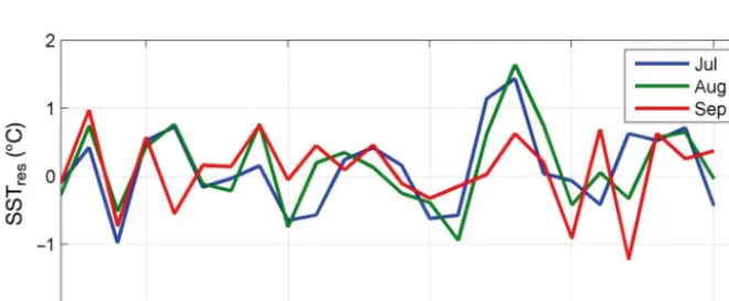
We chose to investigate SST anomalies based on climatologies derived for the period 1971 to 2000 and applied to the time period 1982 to 2010, when all SST data sets are available for comparative purposes. For ecologists with interests in responses to climate change, and seeking to choose a particular SST data-base, temporal and spatial patterns inherent to the data should be considered and the physical and bio-logical datasets should be on matching scales. Here, the assumption that Norwegian Sea SST is an impor-tant indirect driver of the growth condition of salmon permitted comparisons amongst 4 different datasets that describe the ocean temperature within the sur-face mixed layer. Although each grid point for OISST V2, HadISST and ERRST V3b represents an area of ocean surface, the use of kernels can be recommended if the effective ecological spatial scale mar -kedly exceeds the grid size. If no gridded fields are available, fixed point data (here, OWS Mike) can be used as a representation of an area, but their associ-ated limitations almost inevi ta bly will preclude valid applications because oceano graphic scale also has to be considered when defining the spatial area of interest. One possible way forward with gridded fields would be a prior in ves tigation of the temporal variability of SST residuals for spa tial correlation; thus, for example, high variability would indicate restricted spatial autocorrelation and that the grid point perhaps is at the border of 2 distinct regimes. Autocorrelation might easily be allowed for either by de-trending the data or by adjusting df for correlation analyses (Brown et al. 2011). While the latter approach retains more information, an adequate number of observations is needed to account for autocorrelation and this may constrain its ap pli ca tion to short time-series that are highly autocorrelated. Here, the PP method was not able to deliver a meaningful result be -cause the salmon time-series were too short (NWr= 15). Resid-ual analysis of de-seasoned and de-trended SST time-series can represent the other extreme, in that much information can be lost by the preparatory pro -cessing. Residuals calculated for either end of a time-series are more error prone because they are very sensitive to the smooth-ing method used. Nonetheless, in providing a very conservative Fig. 7. Residuals from mean monthly sea surface temperature (SST) anomalies (for

July, August and September) for the OISST V2 dataset at OWS Mike. In 1988, 1989 and 1990, these 3 months reflected essentially the one within-year SST anomaly. This illustrates that, due to slow temporal changes in SST, consecutive anomalies and residuals can be correlated, and comparisons involving them are likely to produce similar results. This has implications for setting the number of tests in applying e.g.

approach, any significant results arising from resid-ual analysis can be considered well supported and the method also is readily applicable to shorter time-series. In the present case, the extension of the SP salmon time-series by an additional year did slightly alter the smoothing of the end of the time-series, but had no influence on the primary significant correla-tion detected by Todd et al. (2008) for January (lag −6 mo; Fig. 6).

Recommendations

For studies similar to the present we endorse the use of OISST V2 for time-series dating from 1982. HadISST is recommended for time-series pre-dating 1982, whilst ERSST V3b could be used for spatial and temporal scale correlations beyond the mesoscale, but not on an anomaly level. Time-series should be a de-seasoned and de-trended prior to the calculation of residuals, and significance levels should also be adjusted based on the df. Whilst the resulting time-series may be free of autocorrelation, and classical hypothesis testing thereby appropriate, statistical power of the final correlation analyses might be expected to be reduced using this technique. A final recommendation to maximize stringency in the iden-tification of significant outcomes might be to accept only those correlations that satisfy Bonferroni correc-tion for both the raw data and the residuals.

Acknowledgements. NOAA_ERSST_V3 and NOAA_ OI_

SST_V2 data provided by the NOAA/OAR/ESRL PSD, Boul-der, Colorado, USA, from their Web site at www. esrl. noaa.gov/psd/. The HadISST 1.1 data are available from the Met Office, Hadley Centre through the NCAS British Atmospheric Data Centre (BADC) from http:// badc. nerc. ac.uk/view/badc.nerc.ac.uk__ATOM__dataent_hadisst. Data from the OWS Mike are available from the EuroSITES Project (www.eurosites.info). The authors acknowledge the support of the MASTS pooling initiative (The Marine Alliance for Science and Technology for Scotland) in the completion of this study (grant reference HR09011).

LITERATURE CITED

Bailleul F, Charrassin JB, Monestiez P, Roquet F, Biuw M, Guinet C (2007) Successful foraging zones of southern elephant seals from the Kerguelen Islands in relation to oceanographic conditions. Philos Trans R Soc Lond B Biol Sci 362: 2169−2181

Biuw M, Boehme L, Guinet C, Hindell M, and others (2007) Variations in behavior and condition of a southern ocean top predator in relation to in situoceanographic condi-tions. Proc Natl Acad Sci USA 104: 13705−13710 Blackwell BG, Brown ML, Willis DW (2000) Relative weight

(Wr) status and current use in fisheries assessment and

management. Rev Fish Sci 8: 1−44

Boehme L, Lovell P, Biuw M, Roquet F and others (2009) Technical note: Animal-borne CTD-satellite relay data loggers for real-time oceanographic data collection. Ocean Sci 5: 685−695

Box GEP, Jenkins GM, Reinsel GC (2008) Autocorrelation function and spectrum of stationary processes. In: Box GEP, Jenkins GM, Reinsel GC (eds) Time series analysis. John Wiley & Sons, Oxford, p 21−46

Bradshaw CJA, Higgins J, Michael KJ, Wotherspoon SJ, Hindell MA (2004) At-sea distribution of female southern elephant seals relative to variation in ocean surface prop-erties. ICES J Mar Sci 61: 1014−1027

Brown CJ, Schoeman DS, Sydeman WJ, Brander K and others (2011) Quantitative approaches in climate change ecology. Glob Change Biol 17: 3697−3713

Charrassin JB, Bost CA (2001) Utilisation of the oceanic habitat by king penguins over the annual cycle. Mar Ecol Prog Ser 221: 285−297

Chavez FP, Messie M, Pennington JT (2011) Marine primary production in relation to climate variability and change. Annu Rev Mar Sci 3: 227−260

Gammelsrod T, Osterhus S, Godoy O (1992) Decadal varia-tions of ocean climate in the Norwegian Sea observed at Ocean Station Mike (66° N 2° E). In: Dickson RR, Malkki P, Radach G and others (eds) Hydrobiological variability in the ICES area, 1980–1989. ICES Mar Sci Symp 195: 68−75

Genner MJ, Sims DW, Wearmouth VJ, Southall EJ, South-ward AJ, Henderson PA, Hawkins SJ (2004) Regional climatic warming drives long-term community changes of British marine fish. Proc R Soc Lond Ser B Biol Sci 271: 655−661

Genner MJ, Sims DW, Southward AJ, Budd GC and others (2010) Body size-dependent responses of a marine fish assemblage to climate change and fishing over a cen-tury-long scale. Glob Change Biol 16: 517−527

Gomes HR, Goes JI, Saino T (2000) Influence of physical processes and freshwater discharge on the seasonality of phytoplankton regime in the Bay of Bengal. Cont Shelf Res 20: 313−330

Gould J, Roemmich D, Wijffels S, Freeland H and others (2004) Argo profiling floats bring new era of in situocean observations. Eos Trans Am Geophys Union 85: 185−191, doi: 10.1029/2004EO190002

Guinet C, Dubroca L, Lea MA, Goldsworthy S and others (2001) Spatial distribution of foraging in female Antarctic fur seals Arctocephalus gazella in relation to oceano-graphic variables: a scale-dependent approach using geographic information systems. Mar Ecol Prog Ser 219: 251−264

Holm M, Jacobsen JA, Sturlaugsson J, Holst JC (2006) Behaviour of Atlantic salmon (Salmo salarL.) recorded by data storage tags in the NE Atlantic — implications for interception by pelagic trawls. ICES CM 2006/Q: 12, p 1−16

Hughes SL, Holliday NP, Colbourne E, Ozhigin V, Valdi -marsson H, Osterhus S, Wiltshire K (2009) Comparison of

in situtime-series of temperature with gridded sea sur-face temperature datasets in the North Atlantic. ICES J Mar Sci 66: 1467−1479

Jacobsen JA, Hansen LP (2000) Feeding habits of Atlantic salmon at different life stages at sea. In: Mills D (ed) The ocean life of Atlantic salmon: environmental and bio -logical factors influencing survival. Fishing News Books,

Oxford, p 170−192

Jensen AJ, Fiske P, Hansen LP, Johnsen BO, Mork KA, Næsje TF (2011) Synchrony in marine growth among Atlantic salmon (Salmo salar)populations. Can J Fish Aquat Sci 68: 444−457

Lutjeharms JRE, Walters NM, Allanson BR (1985) Oceanic frontal systems and biological enhancement. In: Sieg -fried WR, Condy PR, Laws RM (eds) 4th SCAR Symp Antarct Biol. Springer, New York, NY, p 11−21

McClain EP, Pichel WG, Walton CC (1985) Comparative performance of AVHRR-based multichannel sea-surface temperatures. J Geophys Res 90: 11587−11601

Miller RG (1981) Simultaneous statistical inference. Springer, New York, NY

Mills KE, Pershing AJ, Sheehan TF, Mountain D (2013) Climate and ecosystem linkages explain widespread declines in North American Atlantic salmon populations. Glob Chang Biol 19: 3046−3061

Osafune S, Yasuda I (2012) Numerical study on the impact of the 18.6-year period nodal tidal cycle on water masses in the subarctic north pacific. J Geophys Res 117: C05009 Pollard RT, Lucas MI, Read JF (2002) Physical controls on biogeochemical zonation in the southern ocean. Deep-Sea Res II 49: 3289−3305

Pyper BJ, Peterman RM (1998) Comparison of methods to account for autocorrelation in correlation analyses of fish data. Can J Fish Aquat Sci 55: 2127−2140

Rayner NA, Parker DE, Horton EB, Folland CK and others (2003) Global analyses of sea surface temperature, sea ice, and night marine air temperature since the late nine-teenth century. J Geophys Res 108: 4407 doi: 10.1029/ 2002JD002670

Reynolds RW (1988) A real-time global sea surface tem -perature analysis. J Clim 1: 75−86

Reynolds RW, Chelton DB (2010) Comparisons of daily sea surface temperature analyses for 2007–08. J Clim 23: 3545−3562

Reynolds RA, Smith TM (1995) A high-resolution global sea surface temperature climatology. J Clim 8: 1571−1583 Reynolds RW, Rayner NA, Smith TM, Stokes DC, Wang WQ

(2002) An improved in situand satellite SST analysis for climate. J Clim 15: 1609−1625

Reynolds RW, Zhang HM, Smith TM, Gentemann CL, Wentz F (2005) Impacts of in situand additional satellite data on the accuracy of a sea-surface temperature analysis for

climate. Int J Climatol 25: 857−864

Rikardsen AH, Dempson JB (2011) Dietary life-support: the food and feeding of Atlantic salmon at sea. In: Aas Ø, Einum S, Klemetsen A, Skurdal J (eds) Atlantic salmon ecology. Wiley-Blackwell, Oxford, p 115−143

Sims DW, Genner MJ, Southward AJ, Hawkins SJ (2001) Timing of squid migration reflects North Atlantic climate variability. Proc R Soc Lond Ser B Biol Sci 268: 2607−2611 Sims DW, Wearmouth VJ, Genner MJ, Southward AJ, Haw -kins SJ (2004) Low-temperature-driven early spawning migration of a temperate marine fish. J Anim Ecol 73: 333−341

Smith TM, Reynolds RW, Peterson TC, Lawrimore J (2008) Improvements to NOAA’s historical merged land-ocean surface temperature analysis (1880–2006). J Clim 21: 2283−2296

Todd CD, Hughes SL, Marshall CT, MacLean JC, Lonergran ME, Biuw EM (2008) Detrimental effects of recent ocean surface warming on growth condition of Atlantic salmon. Glob Chang Biol 14: 958−970

Ward P, Whitehouse M, Meredith M, Murphy E and others (2002) The southern Antarctic Circumpolar Current front: physical and biological coupling at South Georgia. Deep-Sea Res I 49: 2183−2202

Woodruff SD, Worley SJ, Lubker SJ, Ji ZH and others (2011) ICOADS release 2.5: extensions and enhancements to the surface marine meteorological archive. Int J Climatol 31: 951−967

Wright SP (1992) Adjusted p-values for simultaneous infer-ence. Biometrics 48: 1005−1013

Xing XG, Claustre H, Blain S, D’Ortenzio F, Antoine D, Ras J, Guinet C (2012) Quenching correction for in vivo

chlorophyll fluorescence acquired by autonomous plat-forms: a case study with instrumented elephant seals in the Kerguelen region (Southern Ocean). Limnol Oceanogr Methods 10: 483−495

Xue Y, Smith TM, Reynolds RW (2003) Interdecadal changes of 30-yr SST normals during 1871-2000. J Clim 16: 1601−1612

Yasunaka S, Hanawa K (2011) Intercomparison of historical sea surface temperature datasets. Int J Climatol 31: 1056−1073

Yndestad H (1999) Earth nutation influence on system dynamics of Northeast Arctic cod. ICES J Mar Sci 56: 652−657

Editorial responsibility: Jake Rice, Ottawa, Ontario, Canada

Submitted: March 20, 2014; Accepted: August 29, 2014 Proofs received from author(s): November 15, 2014

➤

➤

➤

➤

➤

➤

➤

➤

➤

➤

➤

➤

➤

➤

➤

➤

➤

➤