Munich Personal RePEc Archive
Does Higher Education Increase Hedonic
and Eudaimonic Happiness?
Nikolaev, Boris
Baylor University
2016
Online at
https://mpra.ub.uni-muenchen.de/78438/
Does Higher Education Increase Hedonic and
Eudaimonic Happiness?
Boris Nikolaev ∗
Oxford College of Emory University
May 29, 2016
Abstract
An increasing number of studies suggest that the relationship between higher education and sub-jective well-being (SWB) is either insignificant or negative. Most of these studies, however, use life satisfaction as a proxy for SWB. In this study, using longitudinal data from the Household Income and Labor Dynamics in Australia (HILDA) survey, I examine the link between higher education and three different measures of subjective well-being: life satisfaction and its different sub-domains (eval-uative), positive and negative affect (hedonic), and engagement and purpose (eudaimonic). Three substantial results emerge: (1) people with higher education are more likely to report higher levels of eudaimonic and hedonic SWB, i.e., they view their lives as more meaningful and experience more positive emotions and less negative ones; (2) people with higher education are satisfied with most life domains (financial, employment opportunities, neighborhood, local community, children at home) but they report lower satisfaction with the amount of free time they have; (3) the positive effect of higher education is increasing, but at a decreasing rate; the SWB gains from obtaining a graduate degree are much lower (on the margin) compared to getting a college degree.
Keywords: Subjective Well-being, Returns to Education, Panel Estimation
JEL Classification Numbers: I0, J24, I21, I31.
1
Introduction
Education is widely acknowledged as one of the most important investments in human
capital that helps individuals develop a multitude of skills that provide many tangible and
intangible benefits. Hundreds of academic studies in different times and places show that
better educated people live longer and healthier lives, are more likely to marry successfully,
experience higher quality of interpersonal relationships, and have more opportunities on
the labor market (Oreopoulos and Salvanes, 2011). Yet, an increasing number of studies
in the emerging field of happiness economics have documented an insignificant relationship
between higher education and subjective well-being with some studies suggesting that the
relationship is strictly negative (Clark and Oswald,1995;Shields et al.,2009;Powdthavee,
2010; Nikolaev, 2015). In a recent review of the happiness literature, Veenhoven (2010)
concludes that school education is the only capability that does not seem to make people
happier.
There are several possible explanations for this puzzling observation. The most
com-mon one is that higher education can make people more ambitious which might reduce life
satisfaction since higher aspirations are more difficult to fulfill (Clark and Oswald,1995).
College graduates, for instance, are known to experience higher levels of stress related to
unemployment than their less educated counterparts. It is also possible that less happy
people are more likley to pursue higher education, which drives the results in many
cor-relational studies (Veenhoven, 2010). Another possible story is that most studies estimate
reduced form happiness regressions that often control for variables such as income, health,
and marital status and thus close these channels through which education may contribute
positively to higher levels of SWB (Powdthavee et al., 2015). A more recent explanation
suggests that people are willing to trade off some of their overall happiness for an upward
trajectory in life (Nikolaev and Rusakov,2015). Finally, it is also likely that people pursue
higher education for the sake of social status. Nikolaev(2016), for example, finds that
peo-ple with relatively higher education within their reference group report much higher levels
of life satisfaction.
Yet, it is by now widely recognized that SWB has multiple dimensions which are only
weakly correlated with each other (Kahneman and Deaton,2010;Stiglitz et al.,2009). More
generally, there are three different types of SWB measures: (1) evaluative, (2) hedonic, and
(3) eudaimonic. The first one, which is most commonly used in happiness studies and is
usually proxied with survey questions on life satisfaction, reflects a cognitive evaluation of
one’s life. Here, individuals are asked to make statements about how their life is going in
general (or as a whole). A second type of measure has to do with the balance between
positive and negative emotions in people’s daily lives. This type of SWB is often called
hedonic or affective well-being (Diener et al.,2002). Lastly, there are non-hedonic/evaluative
measures, which usually capture meaning, purpose, or accomplishment, which are often
called eudaimonic (Clark,2016). These measures reflect people’s innate psychological needs
for belonging, autonomy, self-esteem, or mastery and are sometimes related to Maslow’s
hierarchy of needs (Maslow,1943) or the theory of self-determination (Deci and Ryan,2002).
Seligman(2012), for example, argues that well-being, or what he calls authentic happiness,
is a function of these three different types of SWB. He puts an emphasis on the eudaimonic
happiness, which according to him is the most lasting one. It is also important to mention
that while most economists recognize that SWB is an important argument in the utility
function, they also believe that there are many others. In that sense, people constantly make
trade-offs between their SWB, and its different dimensions (positive emotion vs meaning)
and other aspects of their lives such as achievement or their personal relationships.
In this paper, I contribute to this line of research in three ways. First, I provide a
number of empirical tests using longitudinal data from the HILDA dataset on all three types
of SWB: (1) evaluative, (2) hedonic, and (3) eudaimonic. Second, following the approach
proposed byVan Praag et al.(2003), I furthermore examine the relationship between higher
education and ten different life domain satisfactions (DS). Finally, I investigate the effect for
four different levels of educational attainment – less than high school, high school, college,
and graduate school. Since an increasing number of people pursue advanced degrees today
(beyond a college diploma), it is important to understand the incremental SWB benefits
associated with each level of educational attainment and not just the return from a college
me to control for a large set of confounding variables including personality traits and to use
variation within a person’s lifetime as well as across individuals.
Three substantial results emerge: (1) people with higher education are more likely to
report higher levels of eudaimonic and hedonic SWB, i.e., they view their lives as more
meaningful and experience more positive emotions and less negative ones; (2) people with
higher education are satisfied with most life domains (financial, employment opportunities,
neighborhood, local community, children at home) but they consistently report lower
satis-faction with the amount of free time they have; (3) the positive effect of higher education is
increasing, but at a decreasing rate; the SWB gains from obtaining a graduate degree are
much lower (on the margin) compared to getting a college degree.
These results shed light on some of the previous contradictory empirical findings in the
literature and suggest that higher education has large SWB returns, especially when it
comes to eudaimonic and hedonic happiness. The findings also suggest one possible reason
why more educated people report lower levels of life satisfaction–while people with higher
degrees have more fulfilling and meaningful jobs, they also have less time to enjoy other
aspects of their lives. Finally, the results in this study point to important trade-offs between
these three different types of SWB that people could be making when choosing to go to
college.
2
Theoretical Considerations
The role of education in promoting individual well-being has been widely explored in the
academic literature. Most of the earlier studies examine the indirect effect of education
on happiness through the income channel. Starting with Becker (2009), the emphasis of
economic analysis has been on the financial return from schooling.1
The basic assumption
is that higher income leads to greater consumption which increases individual utility. A
large number of studies using different estimation techniques and considering factors such
as intelligence, ability, and family background find that, on average, an additional year of
schooling increases personal income from 7 to 12 percent (Card,1999).
1
Almost all of these studies are indebted in the human capital earnings model first developed byMincer
More recently, economists have started investigating the effect of education on a variety
of other, non-pecuniary outcomes, such as enjoyment from work, health, marriage, and
par-enting decisions that are also linked to subjective well-being. In a recent study,Oreopoulos
and Salvanes(2011) conclude that these non-pecuniary returns from education are as large
as the pecuniary ones. In this section, I review the literature on the non-pecuniary benefits
which are realized directly by the student.2
2.1 Non-monetary Returns in the Labor Force
An obvious benefit of education is that it facilitates students in the process of self-discovery
and helps them find careers that are a better match for their talents, interests, and
aspira-tions. Another form of non-pecuniary benefit in the labor force is that education provides
individuals with the option to obtain even higher education. Higher educational credentials
usually come with more employment choices. A third benefit is the increased ability to
adjust to changing job opportunities (for example, due to rapid technological change).3
In
this case, adaptability is seen as an output from obtaining a higher degree.
Having a good education, then, increases the likelihood of finding a job and earning
higher income and decreases the reliance on social assistance. The long-term and negative
effect of unemployment on subjective well-being is well-established in the economic literature
(e.g., see Di Tella and MacCulloch (2006)). But more education can also increase the
likelihood of finding not just a job, but a job that is more interesting, meaningful, safer,
more prestigious, and ultimately more enjoyable. Several recent studies find that people
with more education are also more likely to find a more satisfying job, and have greater
autonomy and independence at work (Albert and Davia,2005). Similarly, Oreopoulos and
Salvanes(2011) show that workers with similar backgrounds, but more schooling, have jobs
that offer a greater sense of accomplishment and are more prestigious.
2
In this study, I discuss the private return from education. There is a large literature that is dedicated to the external benefits of education to society. Higher education, for example, is positively correlated with economic growth and development.
3
2.2 Non-monetary Returns Outside of the Labor Force
Even though economist usually focus on the returns of higher education in the labour force,
a great deal of the value of education is realized in terms of better choices and
opportu-nities outside of the labor market. Grossman (2006) provides a more general (theoretical)
framework that outlines how cognitive development generates returns to students in other
domains of life through productive and allocative efficiency. The productive efficiency model
suggests that education teaches students time and resource management skills that allow
them to achieve better outcomes with less resources – more educated people are able to
do more with less. On the other hand, the allocative efficiency model suggests that
educa-tion helps people make better choices which allows them to achieve superior outcomes with
the same level of resources. In this respect, a key non-monetary benefit from additional
education is improvement in physical and mental health.
The most obvious benefit from better health is reduced health care costs and longer life
which may translate into higher productivity and lifetime earnings. But good health can
also increase access to education, jobs, and improve social relations which may also enhance
economic opportunities. The positive association between higher education and health is
well-established in the literature [e.g., see Cutler and Lleras-Muney (2006); Mirowsky and
Ross (2003)]. People with higher education are also more likely to have stronger social
networks and to experience a greater sense of control over their life which is associated with
better health and happiness (Verme,2009). More importantly, the better educated are less
likely to engage in risky personal habits such as smoking and drinking and are more likely
to exercise and get a regular health check-up (Ross and Wu,1995).
Another non-pecuniary benefit from higher education is that well-educated people,
per-haps due to their higher earning potential and higher socio-economic ranking, are more
at-tractive on the competitive marriage market (Becker,1973;Chiappori et al.,2009). Married
people often report significant happiness premium compared to singles (Frey and Stutzer,
2002). Qari (2010), for example, argues that individuals do not fully adapt to the positive
spike in happiness from marriage. He estimates the monetary equivalent of these long-term
There is also abundant evidence that women with more education have fewer children
(Jones et al., 2008). Having fewer children is associated with higher life satisfaction. This
negative correlation is often explained by differences in family structure (White et al.,1986).
For example, having more children is often correlated to more financial dissatisfaction and
more traditionalism in the division of labor. More importantly, educated people tend to be
better parents (Leigh, 1998) and parental education is one of the strongest determinants
of child development. Recent research, for example, suggests that parental education is
correlated with a myriad of positive outcomes – from children’s cognitive development
in early life to their educational attainment and job prospects later in life (Cunha and
Heckman,2009). One explanation of these findings is that more educated people differ in
their parenting styles. For example, better educated parents not only spend more time with
their children, but they are also less likely to discipline them and more likely to encourage
them to pursue new knowledge and to think independently.
Education is also often described as one of the most robust predictors of social capital and
civic engagement (Helliwell and Putnam,2007). Social capital reflects the idea that social
connections – friendships, volunteering, and other relationships – generate value beyond
the intrinsic pleasure that people derive from interacting with others.Recent studies also
show that spending time with family, friends, and colleagues is associated with higher
average levels of positive feelings (Kahneman and Krueger, 2006). But even beyond the
intrinsic pleasure that people derive from spending time with others, social connections
have a positive external effect on individuals and society. Social networks, for example,
provide both material and emotional support in good and bad times. Helliwell et al.(2004)
find that social capital (measured by the strength of family, neighborhood, religious, and
community ties) is independently and robustly positively correlated with life satisfaction,
both directly and through their impact on health.
2.3 Education and Subjective Well-being
Based on the literature review above, it is easy to see why some of the recent empirical
findings that higher education is not significantly or even negatively correlated with SWB
2015). Education, after all, can lead to a more successful, meaningful, and happy life
through variety of economic and non-economic channels.
Of course higher education may come with some negative non-pecuniary returns. For
example, better paid jobs also come with more responsibilities and expectations for improved
performance which may lead to longer work hours and more stress at work. Employees that
work longer hours may find it challenging to balance their work and daily living. Using data
from the General Social Survey,Oreopoulos and Salvanes(2011) point out the tendency for
college graduates to report wanting to spend more time with friends and family. Yet, this
could be because more educated people value family, friendships, and hobbies more than
those who are less educated.
Another negative effect from higher education is the price of unemployment. People
with higher degrees have better jobs and earn higher incomes and losing a job has a higher
economic cost to them. Clark and Oswald (1994) find that better educated people tend
to cope with unemployment less successfully than do those who have lower degrees. In
a separate study, Clark and Oswald (1995) show that more educated people report lower
levels of life satisfaction. One possible explanation of their findings is that education raises
job expectations, which are more difficult to fulfill. Another explanation is that inequality
of income increases with social class, and relative income tends to play an important role
in determining individual happiness. Several other studies also find a negative association
between education and life satisfaction or the absence of a significant relationship between
the two (Clark and Oswald,1995;Shields et al.,2009;Powdthavee,2010;Klein and Maher,
1966;Warr,1992;Blanchflower et al.,1992;Nikolaev,2015,2016). In a review of this
liter-ature from the World Database of Happiness, Veenhoven (2010) concludes that education
does not seem to increase the happiness of pupils.
Other studies, however, report a positive and significant relationship even after
account-ing for some of the indirect channels through which better education may positively affect
well-being such as income, marriage, and health. For example, (Cu˜nado and de Gracia,
2012) study the impact of education on happiness in Spain using individual level data from
the European Social Survey and discover that education has a positive (and direct) effect on
which, as they argue, is a result from acquiring knowledge. Oreopoulos and Salvanes(2011)
find that more schooling leads individuals to make better decisions about health, marriage,
and parenting, and, ultimately, to a happier life. The authors argue that an important
way in which school makes people happy is to make individuals more patient, goal-oriented,
and less likely to engage in more risky behaviors. And, Powdthavee et al. (2015) find that
once you account for the positive effect of higher education on income, health and marriage
outcomes, the overall (both direct and indirect) effect of education on happiness is actually
positive and substantial.
To the best of my knowledge, majority of these previous studies examine the relationship
between education and evaluative happiness, which is most often proxied by life
satisfac-tion. In this study, I complement prior work by examining the link between education and
three different types of SWB, including measures of eudaimonic and hedonic SWB. I
fur-thermore, examine individuals satisfaction from ten different life domains–from satisfaction
with job opportunities to satisfaction with the amount of free time. Thus, the results in
this study provide additional empirical evidence that help better understand the underlying
relationship between higher education and SWB.
3
Data
Data for the analysis were collected from the Household Income and Labour Dynamics in
Australia (HILDA) survey, waves 1-13. The dataset is a large nationally representative
panel that collects annually a wide range of information on respondent’s socio-demographic
characteristics, subjective well-being, labor market participation, and family circumstances.
The final sample consists of 20,143 individuals between 22 and 65 years of age and 126,265
individual-year observations for the period 2001-2013. I choose my sample to include people
22 years or older for two reasons. First, majority of people in the sample have completed
the highest level of educational attainment by the age of 22 (college degree). This mitigates
problems associated with endogeneity since SWB today is less likely to affect the level of
education people obtain in the past. Second, this allows me to exclude people who may be
attainment and as a consequence may not have realized many of the benefits that a higher
degree offers. Nikolaev and Rusakov(2015), for example, shows that the SWB returns from
college education increase with age.
Table 1 provides a complete list and summary statistics for all variables used in this
study. Due to attrition, which arises when a non-random sample of individuals chooses not
to respond, the number of individuals varies from year to year. However, the proportion
of respondents from one wave who successfully re-interview in the next wave is reasonably
high, from a low of 87 percent in wave 2 to a high of 97 percent in wave 9 (Watson and
Wooden,2012). Finally, many of the previous studies that document a negative relationship
between education and happiness use data from the HILDA dataset, which makes it ideal
for testing the hypothesis in this paper (Nikolaev,2015;Powdthavee,2010).
[Table 1 around here]
3.1 Life Satisfaction
The dependent variable, life satisfaction, is collected with the following question: “All things
considered, how satisfied are you with your life?” The scale of possible answers is presented
using a visual aid in which the extreme points of the scale were labeled 0 ‘totally dissatisfied’
and 10 ‘totally satisfied’. In that sense, the question reflects an cognitive assessment
involv-ing evaluative judgment of one’s life as a whole (on the meta level) and requires an effort
to remember and evaluate past experiences. Data on domain satisfactions are collected in
a similar fashion. In this study, I utilize responses to ten separate life domains that include
satisfaction with: (1) employment opportunities, (2) financial satisfaction, (3) amount of
free time, (4) the home in which you live, (5) feeling part of your local community, (6) the
neighborhood you live, (7) how safe you feel, (8) relationship with children, (9) relationship
with partner, and (10) children in household get along with each other. These questions
3.2 Eudaimonic SWB
The HILDA dataset contains a unique module that asks respondents a series of questions
that evaluate their psychological well-being (distress). A number of these questions are
related to concepts of meaning, self-worth, and engagement in daily activities. These
mea-sures, although not perfect, provide a good first approximation for eudaimonic SWB. To
create a measure of eudaimonic well-being, I use the average of the responses to four
differ-ent questions that ask responddiffer-ents to answer how often in the past four weeks they have felt
(1) worthless, (2) hopeless, (3) tired for no good reason, and (4) that everything in life was
an effort. The first two questions are related to the concept of self-worth and meaning while
the latter two to the concept of positive engagement and flow. More specifically, data were
collected with: “The following questions are about your feelings in the past 4 weeks. In the
last four weeks, about how often did you feel...worthless?” with possible answers recoded as
1 ‘all of the time’, 2 ’most of the time’, 3 ‘some of the time’, 4 ‘a little of the time’, and
5 ’none of the time’. The index that I create, then, is increasing in eudaimonic SWB. The
data are available only for waves 7, 9, 11, and 13 of the survey, which limits the sample to
53,182 observations.
3.3 Hedonic SWB
Similarly, the set of questions that assess psychological distress also asks respondents to
evaluate their emotional (hedonic) well-being in the past four weeks. I use the average
of five such questions to calculate a measure of hedonic well-being. These questions use
the format described above and include: (1) feeling sad, (2) feeling restless or fidgety, (3)
feeling nervous, (4) cannot sit still, and (5) cannot calm down. All of these measures are
also measured on a scale from 1 ‘all of the time” to 5 ‘none of the time’ with higher values
reflecting higher emotional well-being (less psychological distress).
Cumulatively, the questions on eudaimonic and hedonic well-being described above are
part the Kessler Psychological Distress Scale (K10), which is measured on a scale of 10 to 50
and was first developed for screening populations for clinical depression and anxiety (Kessler
3.4 Positive and Negative Affect
As an alternative measure of hedonic well-being, I use responses from a separate module
on mental health that include questions about positive and negative feelings that people
experience in their daily lives. Specifically, responses were collected using the following
format: “These questions are about how you feel and how things have been with you during
the past 4 weeks . For each question, please give the one answer that comes closest to the
way you have been feeling. How much of the time during the past 4 weeks...Have you been
a happy person?” The recoded scale of answers ranged from 1 ‘none of the time’ to 6 ‘all of
the time’. The index of positive affect, then, is created as an average of the following: (1)
been a happy person and (2) felt calm and peaceful. Negative affect, on the other hand,
reflects answers to questions about: (1) been a nervous person, (2) nothing could cheer you
up, (3) felt down, (4) felt worn out, and (5) felt tired. Overall, this second set of measures,
positive and negative affect, are closely related to the hedonic measures above and provide
an important robustness test.
3.5 Education
The measure of education is continuos and reflects years of formal education and is imputed
from data that asks respondents to answer what is the highest level of education they have
achieved. A respondent who has completed secondary school, for example, is assumed to
have completed 12 years of education while somebody with a college degree is assumed
to have completed 16 years of education. While we are not measuring the actual number
of years spent obtaining a degree, which can vary with the number of degrees or time
spent studying that did not lead to a degree, this approach is common in the economics
of education literature (Card, 1999). As an alternative measure, I use the highest level of
educational attainment, which is recoded as 1 ‘less than high school’, 2 ‘high school’ 3 ‘some
3.6 Other Controls
There are a number of common socio-demographic variables that are used as controls in this
study. The list of these variables includes: age, marital status, sex, employment situation,
log of labor income, self-rated health, exercise habits, personality traits, and region and
year (wave) dummies. All of these variables also came from the HILDA dataset and are
described in Table 1.
4
Empirical Results
In this section, I first describe the estimation model and then present the main results.
4.1 Model
Even though the dependent variables are measured on a scale (e.g., life satisfaction is
measured from 0 to 10) and require an ordered logit estimation, I use a random-effects
(RE) linear estimator with robust standard errors clustered at the individual level. I do
this for two reasons. First, Kahneman and Krueger (2006) provide extensive evidence for
interpreting survey data on SWB as cardinal and comparable, which is common in sociology
and psychology. Second, Ferrer-i Carbonell and Frijters (2004) show that the results from
OLS and ordered logit regressions hardly ever differ in the context of SWB research. Of
course, an additional benefit of using linear estimates is the practical advantage of
easy-to-interpret marginal effects. Thus, I estimate the following reduced form model which is
common in the happiness literature:
SW Bit=αlogyit+βEducationit+γ′X+ǫit (1)
where i = individual, t=year, andX= k explanatory variables (including age, age squared,
marital status, employment situation, and a logarithmic transformation of personal income,
an idiosyncratic error:
ǫit=νi+µit (2)
whereνi represents individual specific fixed-effects andµi is the usual error term. As
com-mon, the error terms are assumed to be random and not correlated with the explanatory
variables. However, this assumption is likely to be violated, especially when it comes to the
fixed-effects term. For example, each individual may be using his or her own scale when
answering the happiness question, which is unobserved to the researcher. This issue is still
one of the major methodological stumbling blocks in happiness research. Moreover,
unob-served individual specific characteristics such as ability, motivation, or family background
are most likely correlated with both SWB and other explanatory variables such as income
and education.
In the context of longitudinal data, there are two methods to deal with the correlation
of the individual observations over time: (1) random-effects (RE) and (2) fixed-effects (FE)
model. I choose the first approach for several reasons. First, the random-effects estimator is
largely preferred in most branches of applied statistics (Cameron and Trivedi,2009). More
importantly, however, the educational variable does not vary substantially over the course of
most adults lifetime, which makes relying only onwithin individual variation problematic.
In addition,Van Praag and Ferrer-i Carbonell(2008) suggest that the use of RE model
is more appropriate in the context of happiness reserach. This is becauseνi is an unknown
parameter in the FE model that needs to be estimated. This means that for 20,000
individ-uals (as in the case of this study), 20,000 extra parameters (1 extra parameter per person)
need to be estimated. This is hardly what we call a parsimonious model. Even more
im-portantly, using a RE model allows for the possibility of estimating both level and shock
effects. However, by using N individual fixed effects, there is no place for a level effects to
be estimated and only shock effects can be estimated that require significant variation over
time. This, again, is not intuitively reasonable in the case of this study. Finally, using a
RE model also allows me to control for other time-invariant characteristics such as gender
4.2 Main Results
We start the analysis in Table 2 which presents the main results in this paper. The basic
specification includes standard socio-demographic controls for age, age squared, sex, marital
status, employment status, log of personal labor income, and regional and year fixed-effects.
All regressions are estimated using a random-effects estimator with robust standard errors
clustered at the individual level.
The main finding in this table is that people with higher education are more likely to
report higher levels of life satisfaction, eudaimonic, and hedonic SWB (models 1-3). The
results in model 4 and 5 furthermore suggest that more educated people tend to experience
more positive affect and less negative affect in their day to day lives. Finally, model 6 shows
that education is negatively correlated with psychological distress (the summary measure
from the Kessler Psychological Distress Scale). The coefficient on education is statistically
significant in all models, although it is significant only at the 10 percent level in model 1
where the dependent variable is life satisfaction.
[Table 2 around here]
The rest of the coefficients in most estimations also have the expected signs and are
statistically significant which provides confidence in the foundations of the model. For
example, the relationship between happiness and age is found to be non-linear with the
least happy years occurring around the age of 40, and with women, married, employed, and
richer people reporting higher levels of SWB.
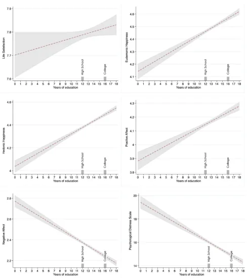
To better understand the magnitude of these relationships, Figure 1 shows the average
predicted value for each one of the SWB measures of interest while holding constant the
other socio-demographic controls in the model at their sample means. The shaded areas in
this figure represent 95 percent confidence intervals for the predictions. The relationship
between higher education and SWB displays a strong and significant correlation in all graphs
with the exception of life satisfaction. The ”average” person,4
for example, who has only a
college degree will report virtually the same level of life satisfaction as their less educated
4
counterpart who has only a high school degree. The effect, however, appears to be far more
substantial when it comes to eudaimonic and hedonic SWB. The average person with a
college degree will report eudaimonic SWB score of close to 4.6 (on a scale from 1 to 5)
while a person with only 8 years of education will score a little over 4.3, a difference of close
to one half of a standard deviation in the dependent variable. To put this in perspective,
the effect of one additional year of schooling is twice as strong as the negative effect from
personal unemployment. The other four graphs display similar patterns.
4.3 Decomposing the Hedonic and Eudaimonic Indexes
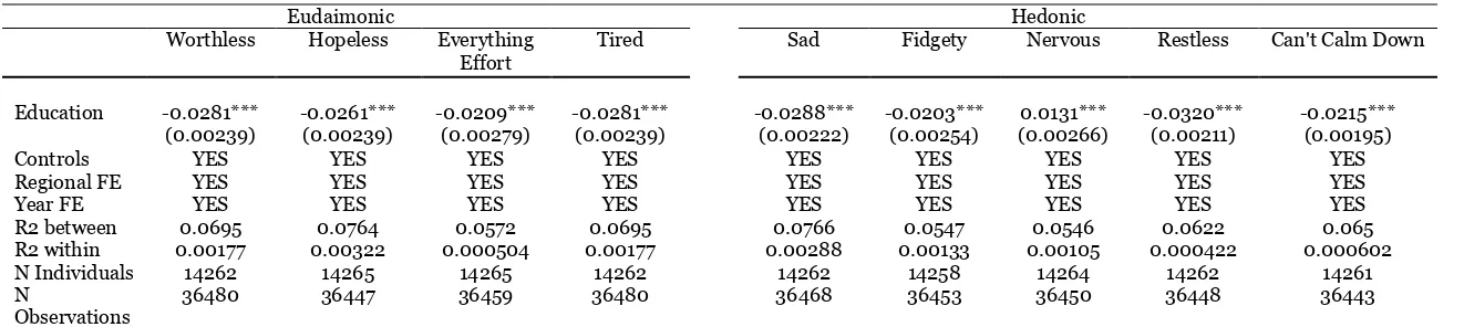
Next, to get even more detailed picture on the relationship between higher education and
SWB, I decompose the two indexes on hedonic and eudaimonic SWB into their more specific
measures and re-estimate the main model from Table 2. The results, which are presented
in Table 3, suggest that people with lower education tend to report being more worthless
and hopeless about their lives. They also report less positive engagement in their daily
activities–they are more likely to be tired for no particular reason and to believe that most
of what they do in life is an effort. On the hedonic side, better educated people are less
likely to report being said, fidgety, restless and not being able to calm down. However,
more educated people are also more likely to report feeling nervous.
[Table 3 around here]
The coefficients on all SWB variables are statistically significant at the 0.000 level and
the magnitude of the relationships are similar to the ones suggested in Table 2.
4.4 Domain Satisfactions
Next, following the approach proposed by Van Praag et al. (2003), I examine how higher
education is associated with ten different domain satisfactions. This approach has previously
been in the context of self-employment (Binder and Coad, 2013). The results, which are
summarized in Table 4, suggest that people with higher education report higher satisfaction
in most life domains. For example, better educated people are more likely to be satisfied
to report higher satisfaction with the neighborhoods they live, being part of their local
community, how safe they feel, and the relationship of their children at home. This is
consistent with the discussion in section 2. Nevertheless, the results in this table also point
out that more educated people report lower life satisfaction with the amount of free time
they have and the home they live in.
[Table 4 around here]
4.5 Results by Gender
Table 5 presents the re-estimation of the main model by gender. The main findings of this
table suggest that the SWB benefits from a higher degree tend to be higher for women.
This is especially true for the measures of eudaimonic and hedonic SWB. The estimated
coefficient for hednic SWB, for example, has a 50 percent larger magnitude. This observation
might help explain the difference in educational attainment between genders that has shifted
over the past few decades. In 1980, for example, there was virtually no difference in the high
school completion rate between females (86 percent) and males (86 percent), but in 2011 the
percentage of females with a high school diploma (91 percent) was higher by four percentage
points than males (87 percent) for the United States. Similarly, in 1980 the percentage of
females (21 percent) with a college degree was three percentage points lower than males (24
percent), but by 2011 significantly more females (36 percent) were graduating college than
males (28 percent). Across the OECD countries, for examples, women with university level
degrees are also twice as likely to find a job as are men (OECD,2012).
4.6 Robustness Check
As a robustness check, I first re-estimate my main model using instead of years of
educa-tion, a recoded variable that measures five levels of education attainment–less than high
school, high school, some college, college, and graduate degree. The so called sheepskin
effect proposes that what matters when it comes to formal education is not the number of
additional years of schooling, but the degree (or certification) that an individual completes.
the main findings so far. They also more clearly show that the positive SWB effect from
higher education is increasing, but at a decreasing rate. For example, the coefficients on
educational attainment from model 2 imply that a high school degree (compared to less
than high school dimploma) increases eidaimonic happiness with close to 0.1 points while
the coefficient on college is only .082 points higher compared to that of a high school degree.
The coefficients on college degree and graduate diploma suggest virtually the same SWB
premium from college and graduate school compared to less than a high school degree.
Similar patterns emerge with respect to the other SWB measures in the table.
[Table 6 around here]
As another robustness check, I re-estimate the main model in Table 2 by adding
ad-ditional controls for health and exercise habits as well as the big five personality traits–
agreeableness, conscientiousness, emotional stability, extroversion, and openness. These
results are reported in Table 7 and significantly limit my sample since the variables on
personality are available only for three years. Even after controlling for these additional
variables, however, I still find that people with higher education are more likely to report
higher levels of eudaimonic and hedonic SWB. They are significantly less likely to report
negative feelings and have psychological distress in their daily lives. However, once I control
for these additional variables, the coefficients on life satisfaction and positive affect become
negative and significant. This suggests that much of the positive effect on life satisfaction
and positive emotions is likely associated with better health and exercise habits or linked
to people’s personality.
[Table 7 around here]
5
Concluding Remarks
An increasing number of studies have documented an insignificant or negative relationship
between higher education and subjective well-being. Majority of these previous studies,
however, use life satisfaction as a proxy for SWB. In this study, I contribute to this line
measures of SWB: (1) evaluative, (2) hedonic, and (3) eudaimonic. I also examine the
relationship between higher education and 10 different life domain satisfactions.
Three substantial results emerge: (1) people with higher education are more likely to
report higher levels of eudaimonic and hedonic SWB, i.e., they view their lives as more
meaningful and experience more positive emotions and less negative ones; (2) people with
higher education are satisfied with most life domains (financial, employment opportunities,
neighborhood, local community, children at home) but they consistently report lower
satis-faction with the amount of free time they have; (3) the positive effect of higher education is
increasing, but at a decreasing rate; the SWB gains from obtaining a graduate degree are
much lower (on the margin) compared to getting a college degree.
These results shed light on some of the previous contradictory empirical findings in the
literature and suggest that higher education has large SWB returns, especially when it
comes to eudaimonic and hedonic happiness. The findings also suggest one possible reason
why more educated people report lower levels of life satisfaction–while people with higher
degrees have more fulfilling and meaningful jobs, they also have less time to enjoy other
aspects of their lives. Finally, the results in this study point to important trade-offs between
these three different types of SWB that people could be making when choosing to go to
college.
6
Bibliography
Albert, C. and Davia, M. A. (2005). Education, wages and job satisfaction. In Epunet
conference. Citeseer.
Alwin, D. F. (1991). Family of origin and cohort differences in verbal ability. American
Sociological Review, pages 625–638.
Becker, G. S. (1973). A theory of marriage: Part i. The Journal of Political Economy,
Becker, G. S. (2009). Human capital: A theoretical and empirical analysis, with special
reference to education. University of Chicago Press.
Binder, M. and Coad, A. (2013). Life satisfaction and self-employment: a matching
ap-proach. Small Business Economics, 40(4):1009–1033.
Blanchflower, D. G. and Oswald, A. J. (2004). Well-being over time in britain and the usa.
Journal of Public Economics, 88(7):1359–1386.
Blanchflower, D. G., Oswald, A. J., and Sanfey, P. (1992). Wages, profits and rent-sharing.
Technical report, National Bureau of Economic Research.
Brist, L. E. and Caplan, A. J. (1999). More evidence on the role of secondary education
in the development of lower-income countries: Wishful thinking or useful knowledge?
Economic Development and Cultural Change, 48(1):155–175.
Cameron, A. C. and Trivedi, P. K. (2009). Microeconomics using stata. College Station,
TX: Stata Press Publications.
Card, D. (1999). The causal effect of education on earnings. Handbook of Labor Economics,
3:1801–1863.
Cascio, E. U. and Lewis, E. G. (2006). Schooling and the armed forces qualifying test
evidence from school-entry laws. Journal of Human Resources, 41(2):294–318.
Chiappori, P.-A., Iyigun, M., and Weiss, Y. (2009). Investment in schooling and the
mar-riage market. American Economic Review, 99(5):1689–1713.
Clark, A. and Oswald, A. (1995). Satisfaction and comparison income. Journal of Public
Economics, 61:359–381.
Clark, A. E. (2016). Swb as a measure of individual well-being. Handbook of Well-being
and Public Policy, forthcoming.
Clark, A. E. and Oswald, A. J. (1994). Unhappiness and unemployment. The Economic
Journal, 104(424):648–659.
Cu˜nado, J. and de Gracia, F. P. (2012). Does education affect happiness? evidence for
spain. Social Indicators Research, 108(1):185–196.
Cunha, F. and Heckman, J. J. (2009). The economics and psychology of inequality and
Cutler, D. M. and Lleras-Muney, A. (2006). Education and health: evaluating theories and
evidence. Technical report, National Bureau of Economic Research.
Deci, E. L. and Ryan, R. M. (2002). Handbook of Self-determination Research. University
Rochester Press.
Dee, T. S. (2004). Are there civic returns to education? Journal of Public Economics,
88(9):1697–1720.
Di Tella, R. and MacCulloch, R. (2006). Some uses of happiness data in economics. The
Journal of Economic Perspectives, 20(1):25–46.
Di Tella, R., MacCulloch, R. J., and Oswald, A. J. (2003). The macroeconomics of
happi-ness. Review of Economics and Statistics, 85(4):809–827.
Diener, E., Lucas, R. E., and Oishi, S. (2002). Subjective well-being. Handbook of Positive
Psychology, pages 63–73.
Ferrer-i Carbonell, A. and Frijters, P. (2004). How important is methodology for the
esti-mates of the determinants of happiness?*. The Economic Journal, 114(497):641–659.
Frey, B. S. and Stutzer, A. (2002). What can economists learn from happiness research?
Journal of Economic Literature, 40(2):402–435.
Frey, B. S. and Stutzer, A. (2010). Happiness and economics: How the economy and
institutions affect human well-being. Princeton University Press.
Green, D. A. and Riddell, W. C. (2003). Literacy and earnings: an investigation of the
interaction of cognitive and unobserved skills in earnings generation. Labour Economics,
10(2):165–184.
Green, F. (2011). Unpacking the misery multiplier: How employability modifies the impacts
of unemployment and job insecurity on life satisfaction and mental health. Journal of
Health Economics, 30(2):265–276.
Grogger, J. (1997). Local violence and educational attainment. Journal of Human
Re-sources, pages 659–682.
Grossman, M. (2006). Education and nonmarket outcomes. Handbook of the Economics of
Education, 1:577–633.
and treatment effects: The mincer equation and beyond. Handbook of the Economics of
Education, 1:307–458.
Helliwell, J. F. and Putnam, R. D. (2007). Education and social capital. Eastern Economic
Journal, 33(1):1–19.
Helliwell, J. F., Putnam, R. D., et al. (2004). The social context of well-being. Philosophical
transactions-royal society of London series B biological sciences, pages 1435–1446.
Inglehart, R., Foa, R., Peterson, C., and Welzel, C. (2008). Development, freedom, and
rising happiness: A global perspective (1981–2007).Perspectives on Psychological Science,
3(4):264–285.
Jones, L. E., Schoonbroodt, A., and Tertilt, M. (2008). Fertility theories: can they explain
the negative fertility-income relationship? Technical report, National Bureau of Economic
Research.
Kahneman, D. and Deaton, A. (2010). High income improves evaluation of life but not
emotional well-being. Proceedings of the National Academy of Sciences, 107(38):16489–
16493.
Kahneman, D. and Krueger, A. B. (2006). Developments in the measurement of subjective
well-being. The Journal of Economic Perspectives, 20(1):3–24.
Kessler, R. C. and Mroczek, D. K. (1995). Measuring the effects of medical interventions.
Medical Care, pages AS109–AS119.
Klein, S. M. and Maher, J. (1966). Education level and satisfaction with pay. Personnel
Psychology, 19(2):195–208.
Layard, P. R. and Layard, R. (2011). Happiness: Lessons from a new science. Penguin UK.
Layard, R., Mayraz, G., and Nickell, S. (2008). The marginal utility of income. Journal of
Public Economics, 92(8):1846–1857.
Leigh, J. P. (1998). Parents’ schooling and the correlation between education and frailty.
Economics of Education Review, 17(3):349–358.
Li, M. (2006). High school completion and future youth unemployment: New evidence from
high school and beyond. Journal of Applied Econometrics, 21(1):23–53.
Machin, S., Salvanes, K. G., and Pelkonen, P. (2012). Education and mobility. Journal of
Maslow, A. H. (1943). A theory of human motivation. Psychological Review, 50(4):370.
Mincer, J. (1974). Schooling, earnings and experience.
Mirowsky, J. and Ross, C. E. (2003). Education, social status, and health. Transaction
Publishers.
Nikolaev, B. (2015). Living with mom and dad and loving it...or are you? Journal of
Economic Psychology, 51:199–209.
Nikolaev, B. (2016). Does other people’s education make us less happy? Economics of
Education Review, 52(2):176–191.
Nikolaev, B. and Rusakov, P. (2015). Education and happiness: an alternative hypothesis.
Applied Economics Letters, pages 1–4.
OECD (2012).OECD Factbook 2011-2012: Economic, Environmental and Social Statistics.
OECD.
Oreopoulos, P. and Salvanes, K. G. (2011). Priceless: The nonpecuniary benefits of
school-ing. Journal of Economic Perspectives, 25(1):159–184.
Pink, D. H. (2011). Drive: The surprising truth about what motivates us. Penguin.
Powdthavee, N. (2010). How much does money really matter? estimating the causal effects
of income on happiness. Empirical Economics, 39(1):77–92.
Powdthavee, N., Lekfuangfu, W. N., and Wooden, M. (2015). What’s the good of
educa-tion on our overall quality of life? a simultaneous equaeduca-tion model of educaeduca-tion and life
satisfaction for australia. Journal of Behavioral and Experimental Economics, 54:10–21.
Qari, S. (2010). Marriage, adaptation and happiness: Are there long-lasting gains to
mar-riage? Journal of Socio-Economics.
Ross, C. E. and Wu, C.-l. (1995). The links between education and health. American
Sociological Review, pages 719–745.
Sacks, D. W., Stevenson, B., and Wolfers, J. (2010). Subjective well-being, income, economic
development and growth. Technical report, National Bureau of Economic Research.
Seligman, M. E. (2012). Flourish: A visionary new understanding of happiness and
well-being. Simon and Schuster.
social characteristics of neighbourhoods. Journal of Population Economics, 22(2):421–
443.
Stiglitz, J. E., Sen, A., and Fitoussi, J.-P. (2009). Report by the commission on the
mea-surement of economic performance and social progress.
Van Praag, B. M. and Ferrer-i Carbonell, A. (2008). Happiness quantified: A satisfaction
calculus approach. Oxford University Press.
Van Praag, B. M., Frijters, P., and Ferrer-i Carbonell, A. (2003). The anatomy of subjective
well-being. Journal of Economic Behavior & Organization, 51(1):29–49.
Veenhoven, R. (2010). Capability and happiness: Conceptual difference and reality links.
The Journal of Socio-Economics, 39(3):344–350.
Verme, P. (2009). Happiness, freedom and control. Journal of Economic Behavior &
Organization, 71(2):146–161.
Warr, P. (1992). Age and occupational well-being. Psychology and Aging, 7(1):37.
Watson, N. and Wooden, M. P. (2012). The hilda survey: a case study in the design
and development of a successful household panel survey. Longitudinal and Life Course
Studies, 3(3):369–381.
Weisbrod, B. A. (1962). Education and investment in human capital. In Investment in
Human Beings, pages 106–123. The Journal of Political Economy Vol. LXX, No. 5, Part
2 (University of Chicago Press).
White, L. K., Booth, A., and Edwards, J. N. (1986). Children and marital happiness why
the negative correlation? Journal of Family Issues, 7(2):131–147.
Yamada, T., Yamada, T., and Kang, J. M. (1991). Crime rates versus labor market
con-ditions; theory and time-series evidence. Technical report, National Bureau of Economic
Appendix
Table 1: Summary Statistics
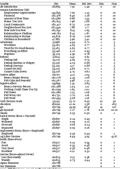
Variable Obs Mean Std. Dev. Min Max Life Satisfaction 182663 7.91 1.49 0 10 Domain Satisfactions (DS)
Employment Opportunities 145,835 7.00 2.41 0 10
Financial 182,576 6.40 2.28 0 10
Amount of Free Time 182,580 6.68 2.53 0 10 Home You Live 182,613 7.96 1.86 0 10 Local Community 182,427 6.73 2.20 0 10 Neighborhood You Live 182,540 7.88 1.77 0 10 How Safe You Feel 182,631 8.15 1.65 0 10 Relationship w Children 106,785 8.42 1.87 0 10 Relationship w Partner 115,879 8.26 2.06 0 10 Children in Household 47,882 5.96 3.42 0 10
Eudaimonic 52966 4.49 0.72 1 5
Worthless 53,182 4.65 0.77 1 5
Tired for No Good Reason 53,182 4.65 0.77 1 5 Everything an Effort 53,148 4.22 0.93 1 5
Hopeless 53,125 4.59 0.78 1 5
Hedonic 52624 4.41 0.61 1 5
Feeling Sad 53,173 4.65 0.73 1 5
Feeling Restless or Fidgety 53,130 4.29 0.86 1 5 Feeling Nervous 53,129 4.17 0.88 1 5 Cannot Sit Still 53,120 4.66 0.71 1 5 Cannot Calm Down 53,128 4.75 0.62 1 5 Positive Affect 161707 4.21 1.04 1 6 Been a Happy Person 162,278 4.43 1.08 1 6 Felt Calm and Peaceful 162,267 3.98 1.22 1 6 Negative Affect 159899 2.32 0.85 1 6 Been a Nervous Person 162,388 2.04 1.11 1 6 Nothing Could Cheer You Up 162,095 1.65 1.02 1 6
Felt Down 162,080 2.15 1.06 1 6
Felt Worn Out 161,732 2.70 1.16 1 6
Felt Tired 162,443 3.08 1.16 1 6
Psych Distress Scale 53235 15.72 6.30 10 50
Education 180292 12.01 2.58 0 18.5
Age 182799 43.95 18.52 14 101
Age Squared 182799 2.27 1.78 0.20 10.20
Female 182799 0.53 0.50 0 1
Marital Status (Base = Married)
Single 182697 0.24 0.43 0 1
Widowed 182697 0.05 0.22 0 1
Divorced 182697 0.06 0.24 0 1
Separated 182697 0.03 0.16 0 1
Employment Status (Base = Employed)
Employed 182799 0.59 0.49 0 1
Log Labor Income 182799 6.49 5.03 0 13.67 Health (Base=Poor)
Fair 161527 0.14 0.34 0 1
Good 161527 0.35 0.48 0 1
Very Good 161527 0.36 0.48 0 1
Excellent 161527 0.12 0.32 0 1
Exercise [Base=Almost Never]
Less than weekly 162813 0.15 0.36 0 1
Weekly 162813 0.73 0.44 0 1
Region Dummies 182788 0 1
Year Dummies 182788 0 1
Table 2: Main Results, Subjective Well-being and Education (1) Life Satisfaction (2) Eudaimonic (3) Hedonic (4) Positive Affect (5) Negative Affect (6) Distress Scale
Education 0.00717* 0.0265*** 0.0284*** 0.0221*** -0.0331*** -0.283***
(0.00382) (0.00226) (0.00195) (0.00254) (0.00215) (0.0200)
Age -0.0664*** -0.0119*** -0.00369 -0.0370*** 0.00676*** 0.0657**
(0.00431) (0.00306) (0.00258) (0.00302) (0.00249) (0.0265)
Age Squared 0.809*** 0.202*** 0.105*** 0.454*** -0.170*** -1.374***
(0.0501) (0.0350) (0.0296) (0.0352) (0.0288) (0.304)
Female 0.138*** -0.0696*** -0.0437*** -0.0650*** 0.153*** 0.546***
(0.0171) (0.0105) (0.00902) (0.0124) (0.0104) (0.0933)
Single -0.409*** -0.134*** -0.123*** -0.117*** 0.0716*** 1.339***
(0.0187) (0.0145) (0.0117) (0.0138) (0.0115) (0.122)
Widowed -0.457*** -0.131*** -0.138*** -0.155*** 0.131*** 1.509***
(0.0818) (0.0428) (0.0413) (0.0476) (0.0401) (0.409)
Divorced -0.519*** -0.165*** -0.135*** -0.0831*** 0.0982*** 1.508***
(0.0313) (0.0221) (0.0182) (0.0204) (0.0168) (0.192)
Separated -0.761*** -0.244*** -0.190*** -0.224*** 0.196*** 2.217***
(0.0345) (0.0284) (0.0226) (0.0223) (0.0178) (0.240)
Employed 0.0291 0.0411*** 0.0161* 0.0150 -0.0387*** -0.279***
(0.0183) (0.0123) (0.00957) (0.0126) (0.0102) (0.0997)
Log Labor Income 0.00909*** 0.0130*** 0.00921*** 0.00676*** -0.00510*** -0.102***
(0.00199) (0.00141) (0.00111) (0.00138) (0.00112) (0.0116)
Regional FE YES YES YES YES YES YES
Year FE YES YES YES YES YES YES
R2 between 0.0746 0.0791 0.0791 0.0321 0.0684 0.0863
R2 within 0.0124 0.00274 0.00189 0.00311 0.00414 0.00297
N Individuals 20143 14254 14228 18992 18951 14267
N Observations 126265 36370 36194 112603 111582 36504
Table 3: Decomposing Hedonic and Eudemonic Indexes
Eudaimonic Hedonic
Worthless Hopeless Everything Effort
Tired Sad Fidgety Nervous Restless Can't Calm Down
Education -0.0281*** -0.0261*** -0.0209*** -0.0281*** -0.0288*** -0.0203*** 0.0131*** -0.0320*** -0.0215*** (0.00239) (0.00239) (0.00279) (0.00239) (0.00222) (0.00254) (0.00266) (0.00211) (0.00195)
Controls YES YES YES YES YES YES YES YES YES
Regional FE YES YES YES YES YES YES YES YES YES
Year FE YES YES YES YES YES YES YES YES YES
R2 between 0.0695 0.0764 0.0572 0.0695 0.0766 0.0547 0.0546 0.0622 0.065
R2 within 0.00177 0.00322 0.000504 0.00177 0.00288 0.00133 0.00105 0.000422 0.000602
N Individuals 14262 14265 14265 14262 14262 14258 14264 14262 14261
N
Observations
36480 36447 36459 36480 36468 36453 36450 36448 36443
Notes: Data HILDA, 2001-2013. Sample includes individuals aged 22-65 years old. Robust standard errors clustered at the individual level reported in parentheses. All models are estimated with a random effects model and include regional and year (wave) fixed effects. The categories male and married are used as base
categories. Statistical significance reported: *** p<0.01, ** p<0.05, * p<0.1
Table 4: Domain Satisfactions
Domain Satisfaction Education (St. error) Controls Regional/Year FE R2 between R2 within Individuals N
Life Satisfaction 0.00717* (0.00382) YES YES 0.0746 0.0124 20143 126265
Employment Opportunities 0.0802*** (0.00603) YES YES 0.251 0.0298 18150 100418
Financial Satisfaction 0.0893*** (0.00548) YES YES 0.189 0.0331 18977 111807
Amount of Free Time -0.0349*** (0.00582) YES YES 0.103 0.0181 18976 111783
The Home You Live -0.00888** (0.00431) YES YES 0.0795 0.00479 18973 111771
Part of Local Community 0.0310*** (0.00520) YES YES 0.0945 0.0101 18973 111716
Neighborhood 0.0126*** (0.00420) YES YES 0.102 0.0100 18971 111736
How Safe You Feel 0.0226*** (0.00416) YES YES 0.114 0.0136 18977 111788
Relationship with Children -0.000367 (0.00586) YES YES 0.0978 0.0238 13567 80732
Relationship with Partner -0.00746 (0.00560) YES YES 0.180 0.0563 16266 89389
Children in Household 0.0409*** (0.00723) YES YES 0.0469 0.0164 10822 51912
Notes: Data HILDA, 2001-2013. Sample includes individuals aged 22-65 years old. Robust standard errors clustered at the individual level reported in
Table 5: Main Results by Gender
Education St. Error Controls Regional FE Year FE R2 between R2 within Individuals N Male
Life Satisfaction 0.00313 (0.00583) YES YES YES 0.0789 0.0137 9803 59963
Eudemonic 0.0243*** (0.00324) YES YES YES 0.0815 0.00385 6748 17020
Hedonic 0.0239*** (0.00288) YES YES YES 0.0772 0.00260 6734 16948
Pos Affect 0.0219*** (0.00376) YES YES YES 0.0386 0.00410 9157 52778
Neg Affect -0.0345*** (0.00306) YES YES YES 0.0597 0.00439 9138 52345
Psych Distress -0.244*** (0.0293) YES YES YES 0.0858 0.00419 6755 17070
Female
Life Satisfaction 0.0125** (0.00508) YES YES YES 0.0715 0.0122 10340 66302
Eudemonic 0.0291*** (0.00316) YES YES YES 0.0732 0.00218 7506 19350
Hedonic 0.0326*** (0.00268) YES YES YES 0.0807 0.00174 7494 19246
Pos Affect 0.0229*** (0.00347) YES YES YES 0.0259 0.00264 9835 59825
Neg Affect -0.0333*** (0.00303) YES YES YES 0.0599 0.00458 9813 59237
Psych Distress -0.322*** (0.0276) YES YES YES 0.0846 0.00256 7512 19434
Table 6: Main Results by Educational Attainment (Degree)
Life Satisfaction Eudemonic Hedonic Pos Affect Neg Affect Psych Distress
High School -0.0189 0.0917*** 0.103*** 0.0638*** -0.0927*** -1.005***
(0.0233) (0.0154) (0.0131) (0.0156) (0.0137) (0.136)
Some College 0.000159 0.150*** 0.165*** 0.101*** -0.151*** -1.632***
(0.0242) (0.0158) (0.0133) (0.0166) (0.0143) (0.139)
College 0.0469 0.151*** 0.182*** 0.106*** -0.178*** -1.763***
(0.0346) (0.0204) (0.0171) (0.0245) (0.0198) (0.176)
Graduate 0.0568 0.175*** 0.190*** 0.161*** -0.221*** -1.898***
(0.0359) (0.0218) (0.0186) (0.0269) (0.0224) (0.189)
Controls YES YES YES YES YES YES
Regional FE YES YES YES YES YES YES
Year FE YES YES YES YES YES YES
R2 between 0.0740 0.0781 0.0771 0.0309 0.0638 0.0847
R2 within 0.0125 0.00271 0.00208 0.00311 0.00415 0.00305
N Individuals 20164 14269 14243 19007 18966 14282
N Observations 126396 36403 36227 112684 111663 36537
Notes: Data HILDA, 2001-2013. Sample includes individuals aged 22-65 years old. Robust standard errors clustered at the
Table 7: Robustness Check (Additional Controls)
Life Satisfaction Eudemonic Hedonic Pos Affect Neg Affect Psych Distress
Education -0.0249*** 0.00861*** 0.0124*** -0.0155*** -0.00713*** -0.115***
(0.00443) (0.00235) (0.00200) (0.00288) (0.00234) (0.0203)
Age -0.0763*** -0.00685** 0.00202 -0.0300*** 0.00396 0.0230
(0.00565) (0.00322) (0.00270) (0.00387) (0.00310) (0.0272)
Age Squared 0.951*** 0.144*** 0.0380 0.388*** -0.154*** -0.872***
(0.0656) (0.0366) (0.0308) (0.0447) (0.0355) (0.310)
Female 0.00386 -0.122*** -0.0830*** -0.165*** 0.197*** 0.997***
(0.0199) (0.0107) (0.00892) (0.0136) (0.0110) (0.0908)
Single -0.386*** -0.0889*** -0.0904*** -0.0998*** 0.0418*** 0.996***
(0.0274) (0.0157) (0.0127) (0.0180) (0.0149) (0.130)
Widowed -0.261*** -0.118** -0.117*** -0.0633 0.0614 1.368***
(0.0869) (0.0466) (0.0412) (0.0533) (0.0422) (0.436)
Divorced -0.600*** -0.152*** -0.129*** -0.112*** 0.117*** 1.464***
(0.0424) (0.0230) (0.0180) (0.0263) (0.0208) (0.189)
Separated -0.847*** -0.245*** -0.176*** -0.232*** 0.246*** 2.184***
(0.0576) (0.0333) (0.0268) (0.0346) (0.0290) (0.277)
Employed 0.0362 0.0564** 0.0112 0.0131 -0.0116 -0.340*
(0.0466) (0.0234) (0.0177) (0.0281) (0.0230) (0.186)
Log Labor Income -0.00330 0.00518** 0.00637*** 0.000796 -0.00610*** -0.0583***
(0.00469) (0.00236) (0.00178) (0.00283) (0.00234) (0.0188)
Fair Health 0.940*** 0.492*** 0.356*** 0.403*** -0.531*** -3.998***
(0.0852) (0.0487) (0.0417) (0.0427) (0.0391) (0.418)
Good Health 1.424*** 0.869*** 0.640*** 0.878*** -0.977*** -7.197***
(0.0834) (0.0470) (0.0407) (0.0421) (0.0383) (0.407)
Very Good Health 1.803*** 1.019*** 0.789*** 1.213*** -1.207*** -8.753***
(0.0837) (0.0470) (0.0407) (0.0425) (0.0386) (0.407)
Excellent Health 2.165*** 1.066*** 0.865*** 1.428*** -1.352*** -9.435***
(0.0857) (0.0478) (0.0415) (0.0448) (0.0403) (0.414)
Exercise (rarely) 0.0821** 0.114*** 0.0842*** 0.0988*** -0.102*** -0.920***
(0.0367) (0.0218) (0.0175) (0.0239) (0.0199) (0.180)
Every week 0.137*** 0.152*** 0.105*** 0.169*** -0.183*** -1.168***
(0.0336) (0.0199) (0.0163) (0.0221) (0.0185) (0.167)
Agreeableness 0.125*** -0.000225 0.00419 0.104*** 0.00111 -0.0172
(0.0121) (0.00695) (0.00577) (0.00792) (0.00665) (0.0591)
Conscientiousness 0.0581*** 0.0651*** 0.0399*** 0.0388*** -0.0469*** -0.490***
(0.00987) (0.00556) (0.00450) (0.00675) (0.00533) (0.0458)
Emotional Stability 0.167*** 0.179*** 0.172*** 0.223*** -0.209*** -1.790***
(0.0100) (0.00586) (0.00467) (0.00668) (0.00546) (0.0479)
Extroversion 0.105*** 0.0713*** 0.0492*** 0.112*** -0.0805*** -0.598***
Openness -0.0360*** -0.0279*** -0.0216*** -0.0146** 0.0213*** 0.244***
(0.00999) (0.00542) (0.00441) (0.00665) (0.00545) (0.0455)
Regional FE YES YES YES YES YES YES
Year FE YES YES YES YES YES YES
R2 between 0.259 0.359 0.371 0.333 0.386 0.401
R2 within 0.0823 0.120 0.120 0.127 0.146 0.143
N Individuals 13964 12163 12135 13914 13845 12194