Attempts to delineate functional regions in Hungary based on commuting data

Attempts to delineate functional regions

in Hungary based on commuting data

Pálóczi, Gábor and Pénzes, János and Hurbánek, Pavol and

Halás, Marián and Klapka, Pavel

University of Debrecen, Catholic University in Ruzomberok, Palacký

University Olomouc

10 October 2016

Online at

https://mpra.ub.uni-muenchen.de/74497/

Attempts to delineate functional regions in Hungary

based on commuting data

Gábor Pálóczi

University of Debrecen, Hungary E-mail: paloczig@gmail.com

János Pénzes

University of Debrecen, Hungary E-mail: penzes.janos@science.unideb.hu

Pavol Hurbánek

Catholic University in Ruzomberok Slovakia E-mail: pavolhurbanek@gmail.com

Marián Halás

Pavel Klapka

The issue of defining functional regions in Hungary is presented in this paper, which contains detailed methodological description with the help of relevant studies from the Czech Republic and Slovakia. The use of Smart’s measure together with the CURDS algorithm and the relatively new concept of trade-off constraint function with four different sets of parameter values provided four optional solutions for this issue, based on the analysis of daily travel-to-work flows from the 2011 census. The resulting regions correspond to the micro-regional level and give valuable additions to the discussion about regionalization. The paper provides basic descriptive statistics for each of the four variants of functional region systems, which enables their overall evaluation (seeing advantages and disadvantages) and mutual comparison (seeing similarities and differences), and thus facilitates an informed debate on future work in functional regionalisation in Hungary carried out with respect to different purposes.

Keywords:

Introduction

introduced into human geography by American geographers such as Philbrick (1957) and Nystuen–Dacey (1961).

The challenge of delineating functional regions is well expressed by Hartshorne (Hartshorne 1939: 275 – cited by Paasi 2009: 4736):

‘The problem of establishing the boundaries of a geographic region presents a problem for which we have no reason to even hope for an objective solution. The most that we can say is that any particular unit of land has significant relations with all the neighbouring units and that in certain respects it may be more closely related with a particular group of units than with others, but not necessarily in all respects’.

Functional, nodal regions can be regarded as open systems. Investigation of the build-up of such systems would first require an analysis of movements (channels along which movements occur), networks, nodes and their hierarchical organisation, acknowledging that this complex system ultimately forms surfaces. According to the orientation of the flows and interactions, four types of functional regions can be identified (oriented, channelled, circular and nodal) besides the random structure (Klapka et al. 2013a).

The objective of the delineation of functional regions is to maximise the ratio of within-region and between-region flows, so the analysis is based on relational dataset (Haggett 1965). During the delimitation process, the horizontal functional relations should be maximised within a region and minimised across its boundaries in order to fulfil the principle of internal cohesiveness and external separation (Smart 1974; Karlsson–Olsson 2006; Farmer–Fotheringham 2011; Klapka et al. 2014).

Administrative or political territorial divisions are not able to reflect the rapid changes in geographical reality, thus correctly defined functional regions can be more appropriate as a geographical tool for normative use (Haggett 1965) than administrative regions.

The interactions most commonly used in functional region delineations are travel-to-work flows, particularly the daily ones. Commuting to work or labour commuting is one of the most frequent and regular movement of the population with daily or rare periodicity. Functional regions based on these relations and flows are referred to as local labour market areas (LLMA) or travel-to-work areas (TTWA).

This study contributes to the discussion of the functional regional system in Hungary by applying a sophisticated regionalisation algorithm using daily travel-to-work flow data. A significant part of the current study emphasises the filtering process of the dataset. Current delimitation is the first attempt to delineate functional units based on the census data with the help of this methodology.

Methods of functional regionalisation

From all possible combinations, the literature tends to favour three approaches to functional regional taxonomy: clustering methods using numerical taxonomy (e.g. Smart 1974) or graph theory procedures (e.g. Nystuen–Dacey 1961; Karlsson–Olsson 2006; Benassi et al. 2015) and the multistage (or rule-based) procedures (e.g. the approach developed by the Centre for Urban and Regional Development Studies [CURDS] in Newcastle, UK – see Coombes et al. 1986 and Coombes–Bond 2008 for more information).

The approach developed by the research team at CURDS became one of the most successful and acknowledged approach to functional regional taxonomy. Considerable European experiences are available from Italy (Sforzi 1997), Slovakia (Bezák 2000; Halás et al. 2014), Spain (Casado-Díaz 2000; Flórez-Revuelta et al. 2008), Belgium (Persyn–Torfs 2011), Poland (Gruchociak 2012), and the Czech Republic (Klapka et al. 2013b; Tonev 2013).

The measure proposed by Smart (1974) [1] is the most frequently used as, mathematically, it is the most appropriate way for the relativisation and symmetrisation of statistical interaction data. It was also used by the second and third variants of the CURDS algorithm (Coombes et al. 1986; Coombes–Bond 2008); its notation is as follows:

Smart’s measure: ,

) T T ( T ) T T ( T ki k jk k 2 i j kj k ik k 2 ij         Σ ∗ Σ + Σ ∗

Σ [1]

where Tij denotes the flow from spatial zone i to spatial zone j and Tji denotes the

flow from j to I; kTik denotes all outgoing flows from i; kTkj denotes all ingoing

flows to j; kTjk denotes all outgoing flows from j; and finally kTkidenotes all ingoing

flows to i.

The second interaction measure was proposed by Coombes et al. (1982) in the first variant of the CURDS algorithm [2], and its notation is as follows:

CURDS measure: ,

) T ( T ) T ( T ) T ( T ) T ( T ki k i j jk k i j kj k ij ik k ij         Σ + Σ + Σ +

Σ [2]

Regionalisation attempts in Hungary

It is important to emphasise that the methodology used in the current analysis represents a new approach among the Hungarian regionalisation attempts even though numerous considerable delimitations were published during the last few decades. This is why it is relevant to overview the previous studies and methods to delineate functional regions in Hungary (some part of these were briefly summarised in a preceding paper about Local Labour Systems – Pénzes et al. 2015).

The issues of territorial division in Hungarian literature are generally discussed by Dusek (2004), Nemes Nagy (2009), and Barancsuk et al. (2014), among others.

As early as the 1960s, the definition of functional regions appeared in the Hungarian human geography (Mendöl 1963), followed by additional researches focusing on the spheres of influences of larger towns (Beluszky 1967). However, this approach avoided the utilisation of commuting data. Functional urban regions were delimited for the whole of Hungary by using commuting relations that assigned each settlement to a single centre and conforming to the hierarchical scheme of the national development concept (Lackó et al. 1978). The country’s territory was segmented based on the public transport connections forming spheres of influences (Szónokyné Ancsin–Szinger 1984) that could also be regarded as functional units. Commuting to work purposes was used as the basis for the dynamic examination of catchment areas (Erdősi 1985). Numerous functional analyses were made for the limited extent of the area – typically for towns and their hinterlands, for example, with the help of inter-urban telephone calls (inter alia Tóth 1974), commercial relations (Kovács 1986) or complex approaches (Timár 1983; Bujdosó et al. 2013).

After the year 2000, as a part of the Regional Polycentric Urban System (RePUS) project, local labour market systems, or the Local Labour Systems (LLSs), were delineated based on the commuting for work data of the 2001 census (Radvánszki– Sütő 2007). Functional Urban Districts (Sütő 2008) were aggregated by utilising these results. The LLS delimitation was updated and modified according to the last census data from 2011 (Pénzes et al. 2015). This approach provided a two-stage model in which the centres were assigned first and then the catchment areas were identified. In this approach, employment centres were in the core of the delimitation, and commuter’s flows were simplified to those oriented towards them. In this respect, the methodology can be regarded as appropriate to identify nodal regions (Klapka et al. 2014). Complex and combined aspects were applied in an extended case study comprising gravity-based theoretical investigations (Hardi–Szörényiné Kukorelli 2014).

role in the study of inter-municipal relations (e.g. Szalkai 2010 and Tóth 2013). Some recent analyses delineated the functional regions based on the online social network (Lengyel et al. 2015).

Methodology of the applied functional regionalisation and

parameters during the procedure

The current delimitation analysis is the first attempt to adapt a methodology tested previously in other Central European countries listed above. This is why we disregarded the detailed description of the methodology. See Klapka et al. (2014) and Halás et al. (2015) for more information on this. However, some of the steps of the calculation need to be reviewed in order to understand the current analysis.

The process of the algorithm’s application can be separated into three stages, which includes four steps and other operations. As part of the first stage, the process starts with the identification of proto-regions (by critical values of the interaction measure), followed by the assignment of remaining spatial zones and finally the assessment of the validity of the solution.

A potential regional core – as part of the interaction measure – must fulfil the criteria of job ratio function (the ratio of total ingoing flows of commuters and total outgoing flows above 0.8) and supply-side (or residence-based) self-containment (ratio of the inner flow and total outgoing flows above 0.5). If these potential cores do not fulfil the criteria, they are identified again based on the mutual relations between them and the value of the interaction measure. This iterative process is repeated until every basic spatial zone is attached to some of the proto-regions. The resulting set of cores and multiple cores is considered as a set of the proto-regions.

Constraint function is used in the following step to set a minimum size and self-containment criteria for the resulting regions. The constraint function is an essential part of the regionalisation algorithm and determines which regions will be maintained and will appear in the resulting regionalisation through the optimisation of the size and self-containment. The constraint function controls these two parameters of the resulting regions and the so-called trade-off between them.

At the same time, the minimum size of the functional region is modifiable. The size of a region can be defined by different criteria. The most general feature of a region is its population size, which is a standard and easily accessible indicator.

The constraint function applied in the current research has the form of a continuous curve (Figure 1), and its shape is determined by four parameters that can be easily set by the user: the upper and lower size limits and the upper and lower self-containment limits (Klapka et al. 2014). The referred methodology of the continuous constraint function is a modified version of the formula –see Halás et al. (2015) for details.

Plotting the resulting regions on a graph is the following step as part of the delineation process. Each region, according to the values of its size and self-containment, can be plotted on an x–y graph as a point (β1 and β2 are lower and upper

limits of the self-containment; β3 and β4 are lower and upper limits of the size in Figure

1). Regions will appear in the upper-right part of the graph from the curve of the constraint function. In practice, the plotting of regions on the graph provides a refinement tool that can help identify more appropriate values for the parameters.

Figure 1

Continuous constraint function

Source: Halás et al. 2015, Figure 3.

The refinement process of testing parameters should start with lower values of size and self-containment. The algorithm produces more regions when smaller parameter values β1–β4 are used, but their position on the x–y graph and knowledge

of the settlement and regional system of a given territory help to make an informed decision as to which regions should be eliminated by setting the size and self-containment parameters to higher values. A graphical assessment of the results can help identify the course and position of the constraint function on the graph. If there is a significant gap in the field of points, that is an area with relatively small density of points, then it is the area of discontinuity of the size and self-containment values of the individual regions, in which a new trade-off constraint function can be located

β1

β4 β3

β2

Employed residents

Sel

f-c

on

ta

in

me

nt o

f re

gio

n re

si

dent

without placing it too close to the size and self-containment values of too many regions. This concept is similar to the one behind the graphical cluster analysis methods or behind the methods for identification of natural breaks in data distribution (e.g. for choropleth map intervals).

Dataset and data corrections within the analysis

The analysis was based on the commuting dataset of the Hungarian census in 2011 carried out by the Central Statistical Office (for the characteristics of the commuting, see Kiss–Szalkai 2014). The survey was realised using harmonised international methodology in which commuting data were derived from the residence and locality of the workplace. The dataset contains aggregated data for the level of settlements (not personal microdata).

Some modifications were necessary. First of all, employees working abroad (83,822) and in more or changing localities (153,410) were filtered out. The districts of Budapest and existing commuting relations were unified. The dataset contains relations that do not conform to the possibility of daily commuting, because of great geographical distance and inadequate transport connections (similar errors were indicated in the Czech dataset as well – see Tonev 2013). In order to use an appropriate value as criteria, the relating literature was necessary to be overviewed.

There is characteristic distribution in the time of travelling, with daily periodicity regarded as constant in time and space since the Neolithic period (Marchetti's constant), apart from the location, way of travelling and other different conditions in the lifestyle. Regional scale analyses since the 1960s defined the characteristic travel time as 1.1–1.3 hours per day (e.g. Zahavi 1976). This suggests that increasing travelling speed is accompanied by increasing travelling distance instead of time-saving. Newest results tend to confute theories about travel time budget (Barthélemy 2011). As a consequence, universal travelling distance or time cannot be determined expressly as a threshold for daily commuting in a given relation.

Commuting with outstanding distance or time is called extreme commuting. The definition of extreme commuting is varied country by country – it is 100 miles (167 km) for the United States, 50 miles (83 km) for the United Kingdom, 100 km for Sweden and Norway, according to the European long-distance travel mobility survey (Vincent-Geslin–Ravalet 2016). Five to ten per cent of the active European population is assumed to commute more than two hours per day, at least three days a week on average (Lück–Rupperthal 2010).

It is important to emphasise that modelled travelling time is generally lower than the real values, as the optimised conditions were calculated using the maximum legal speed, and quality of road infrastructure or traffic jams were not considered. At the same time, commuters using public transport facilities must necessarily expect even greater travelling time (disregarding some main railways where public transport is competitive against individual transport).

Figure 2

Relative frequency of travelling time and number of relations

Source: Calculated by the authors based on the census dataset.

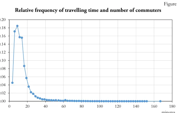
In order to separate the daily and weekly commuting, the relative frequency of the relations between settlements and number of commuters was analysed in the context of travelling time and distance. Travelling time and the number of relations represent a characteristic peak at five minutes of travelling time in the frequency followed by a steep increase (Figure 2). The curve flattens at 40 minutes of travelling time, and commuting became incidental from 90 minutes. Additional features regarding commuters are provided by the numbers in the context of travelling time. It is clear that large-scale commuting radically decreases between the 15 and 20 minutes interval of travelling time and becomes marginal after 40 minutes of travelling time (Figure 3). The most intensive sphere of employment centres can be generally delimited at the 20 minutes travelling time isochron.

Travelling distance was also analysed. The relative frequency of the relations represented a similar distribution to the previous ones. The maximum distance value was 10 km, presenting a steep increase after. However, the number and ratio of relations was regarded as significant between 50 km and 100 km (Figure 4). At the same time, the number of commuters was negligible over 50 km (Figure 5).

0.00 0.02 0.04 0.06 0.08 0.10 0.12

0 20 40 60 80 100 120 140 160 180

Figure 3

Relative frequency of travelling time and number of commuters

Source: Calculated by the authors based on the census dataset.

Figure 4

Relative frequency of travelling distance and number of relations

Source: Calculated by the authors based on the census dataset.

0.00 0.02 0.04 0.06 0.08 0.10 0.12 0.14 0.16 0.18 0.20

0 20 40 60 80 100 120 140 160 180

minutes

0.00 0.01 0.02 0.03 0.04 0.05 0.06 0.07 0.08 0.09 0.10

0 20 40 60 80 100 120 140 160 180 200 220 240 260 280 300

Figure 5

Relative frequency of travelling distance and number of commuters

Source: Calculated by the authors based on the census dataset.

According to the listed features, commuters who were non-daily commuters with place of residence further than 100 km and travelled 90 minutes by car from their place of work were filtered out of the matrix. These thresholds ensured the involvement of not only the most intensive part of the commuting but also the considerable relations assumed as daily periodicity. As the result of this approach, weak connections in terms of network analysis were also involved in the investigation. Relations of over 90 minutes (hypothetically, three hours of travelling per day) and a 100-km distance were assumed as non-daily commutes.

The accessibility and distance matrix was created based on the road network layer of Geox Ltd. from 2013. Travelling time and distance were optimised to the quickest solution between settlements based on the maximum speed of personal cars by running the ArcGIS Network Analyst application (Tóth 2014). Before filtering, the commuting matrix contained 84,747 flows (directional pairs of settlements between which at least one person commutes) and 3,705,491 interactions (commuters); after the filtering, it contained only 70,459 flows (83.14%) and 3,660,953 interactions (89.80 %), of which the inner (within a settlement) commuting amounts to only 3,151 flows (0.04 % of the filtered matrix), but up to 2,545,198 interactions (69.52 % of the filtered matrix), i.e. persons having both residence and employment in the same settlement.

Daily and non-daily periodicity commuting could be detected using microdata of the census, but it was not possible to analyse this case in this way.

0.00 0.02 0.04 0.06 0.08 0.10 0.12 0.14 0.16 0.18

0 20 40 60 80 100 120 140 160 180 200 220 240 260 280 300

Results of the analysis by the case study of Hungary

The algorithm was run four times (1, 2, 3a and 3b versions) based on the commuting dataset using four different sets of parameter values pertaining to the size and self-containment of the regions – in the following, the resulted variants of the regional system are denoted as ‘FRD’ standing for functional regions based on daily interactions (Figure 6). The first run resulted in a general overview of the features of potential functional regions in the Hungarian settlement system due to the set of very small parameter values. During subsequent runs of the algorithm, regions that did not meet the criteria set by the constraint function were dissolved into individual settlements/municipalities and then assigned to other regions (a small village – Gagyapáti – was not assigned to any region because of its local labour isolation). The decrease in the number of functional regions resulted in an increase in their average size regarding the number of settlements and number of employed residents (Table 1).

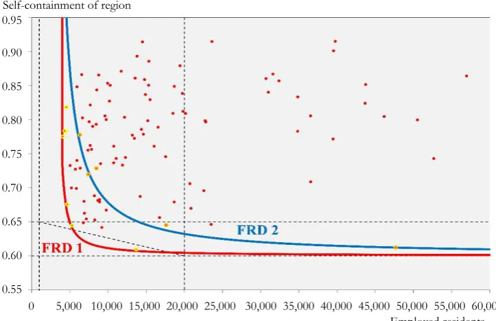
Figure 6

Use of the constraint function on x–y graph by the example of FRD 1 and 2

Source: Calculated by the authors based on the census dataset.

The algorithm provides contiguous regions without the need for further adjustments with several insignificant exceptions (the step of elimination exclave and enclave settlements is not part of the present analysis).

In the second variant, the constraint function is moved up and right to the most distinct visual gap within the red dots in the graph (Figure 6). The modification of the

Employed residents Self-containment of region

0.95

0.90

0.85

0.80

0.75

0.70

0.65

0.60

0.55

parameters in creating a new trade-off constraint function curve (blue line in Figures 6 and 7 with parameters β1=0.60, β2=0.65, β3=3,000 and β4=125,000) served as basis

for the new functional region system FRD 2 with medium-size regions (blue dots in Figure 7). Twenty-four functional regions were present between the red and blue curves. The heuristic character of the methodology is indicated by the fact that Tokaj FR and Szentgotthárd FR (the two orange-red dots closest to the blue line in the left part of Figure 6) might have made it to FRD 2 and/or Komárom FR, Tiszavasvári FR and Vác FR (the other three orange-red dots relatively near the blue line in Figure 6) might have not made it to FRD 2, only if slightly different parameters for the new trade-off constraint function curve were chosen. Subjective decisions appear during the acceptance of the parameters.

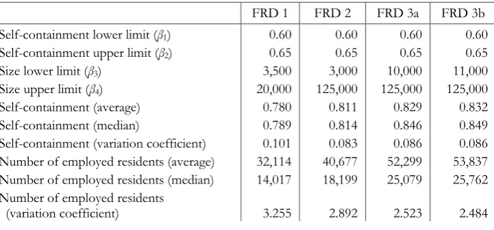
Table 1

Parameters of the constraint function in the case of variants

FRD 1 FRD 2 FRD 3a FRD 3b

Self-containment lower limit (β1) 0.60 0.60 0.60 0.60

Self-containment upper limit (β2) 0.65 0.65 0.65 0.65

Size lower limit (β3) 3,500 3,000 10,000 11,000

Size upper limit (β4) 20,000 125,000 125,000 125,000

Self-containment (average) 0.780 0.811 0.829 0.832

Self-containment (median) 0.789 0.814 0.846 0.849

Self-containment (variation coefficient) 0.101 0.083 0.086 0.086

Number of employed residents (average) 32,114 40,677 52,299 53,837

Number of employed residents (median) 14,017 18,199 25,079 25,762

Number of employed residents

(variation coefficient) 3.255 2.892 2.523 2.484

Source: Calculated by the authors based on the census dataset.

Table 2

Basic features of the function regions in the case of variants

Feature FRD 1 FRD 2 FRD 3a FRD 3b

Number of functional regions 114 90 70 68

Average number of settlements in the FRs 28 35 45 46

Maximum number of settlements in the FRs 129 137 201 201

Minimum number of settlements in the FRs 1 1 5 5

Average number of employed residents 32,504 41,172 52,935 54,492

Maximum number of employed residents 1,190,256 1,196,851 1,196,851 1,196,851

Minimum number of employed residents 3,689 5,917 12,185 13,586

Weight of the centre (average, %) 60 58 54 53

Weight of the centre (maximum, %) 100 100 88 88

Weight of the centre (minimum, %) 13 20 24 24

According to the third variant, the constraint function is moved up and right to the most distinct visual gap again (just slightly to the right of the red-blue dot representing Kunszentmárton FR in Figure 7). As the most distinct visual gap has two dots (representing the Mezőkövesd FR and Nyírbátor FR orange-blue dots in Figure 7) in its centre this time, two variants of the FR system with large-sized regions are proposed (FRD 3a and 3b). FRD 3a preserves the two mentioned functional regions (dark green line with parameters β1=0.60, β2=0.65, β3=10,000 and β4=125,000), whereas FRD 3b (light green line with parameters β1=0.60, β2=0.65, β3=11,000 and β4=125,000) does not contain these two functional regions (Cegléd

FR, represented by the third orange-blue dot near the green lines in Figure 7, remained undissolved). Settlements from Mezőkövesd FR were primarily included into Eger FR and partly into Tiszaújváros FR. Settlements from Nyírbátor FR became part of Mátészalka FR (except for Ófehértó; Figures 10 and 11).

The largest functional regions integrating more than 100 settlements were Budapest FR and Pécs FR as the result of the first variant (FRD 1; Table 3). The modified parameter caused a significant increase in the size of the functional regions in the territories with micro and small villages. Zalaegerszeg FR in the second variant (FRD 2) and Miskolc FR and in the third and fourth variants (FRD 3a and 3b) also surpassed the number of 100 settlements. Pécs FR was the largest region by number of settlements after integrating the remaining parts of Komló FR, Szigetvár FR, and Siklós FR.

Figure 7

Use of the constraint function on x–y graph by the example of FRD 2, 3a and 3b Self-containment of region

0.95

0.90

0.85

0.80

0.75

0.70

0.65

0.60

Table 3

Distribution of the functional regions and participation of persons employed locally categorised by number of persons employed locally

Categories by number employed

residents

Number of functional regions Percentage of the total number of _{employed residents in Hungary}

FRD 1 FRD 2 FRD 3a FRD 3b FRD 1 FRD 2 FRD 3a FRD 3b

1,000,000– 1 1 1 1 32.1 32.3 32.3 32.3

100,000–999,999 3 3 5 5 8.9 8.9 14.9 14.9

50,000– 99,999 9 11 10 10 18.0 21.9 19.5 19.8

20,000– 49,999 21 22 27 27 18.8 18.9 21.6 22.0

10,000– 19,999 36 37 27 25 14.2 14.7 11.7 11.0

– 10,000 44 16 0 0 7.9 3.3 0.0 0.0

Total 114 90 70 68 100 100 100 100

Source: Calculated by the authors based on the census dataset.

Budapest FR was unambiguously the largest territory in light of the number of employed residents followed by Debrecen FR, Székesfehérvár FR, and Miskolc FR (in the first parameter variant – FRD 1). The size of Pécs FR and Szeged FR also exceeded 100,000 employed residents in the FRD 3a and FRD 3b variants. The number and proportion of the smaller functional regions (less than 20,000 employed residents) shrank significantly as the critical parameter values increased from the first to the fourth variant.

Debates about the most appropriate version of these delimitations and comparative spatial analysis with other territorial divisions (administrative or statistical units) were not involved in the current study. These issues might be the most important objectives of further studies.

Conclusions

In the analysis, the Smart’s measure and second variant of the CURDS algorithm were used. Optimisation and tests could be conducted using the modification of the size (number of employed residents) and self-containment of regions. The usage of the continuous constraint function allowed the consideration of the trade-off between the two parameters. The only subjective components within the whole complex procedure were the choices of the exact position of gap within points on the graph and of the exact position of the trade-off function curve within that gap. Except for that, the method provided precise quantitative results that facilitated informed decisions with respect to the desired scale of functional regionalisation. The Hungarian results provide the possibility to continue the discussion about the delimitation of micro-regional level territorial units.

Acknowledgement

This research was supported by the Slovak Scientific Grant Agency VEGA project no. 1/0275/13 ‘Production, verification and application of population and settlement spatial models based on European land monitoring services’.

Figure 8

Functional regions in 2011 by the FRD 1 variant

Figure 9

Functional regions in 2011 by the FRD 2 variant

Source: Edited by the authors based on the census dataset.

Figure 10

Functional regions in 2011 by the FRD 3a variant

Figure 11

Functional regions in 2011 by the FRD 3b variant

Source: Edited by the authors based on the census dataset.

REFERENCES

BARANCSUK,Á.–GYAPAY,B.–SZALKAI,G. (2014): Theoretical and Practical Possibilities of Lower-Medium-Level Spatial Division. Regional Statistics 4 (1): 76–99.

BARTHÉLEMY,M. (2011): Spatial networks. Physics Reports 499: 1–101.

BARTUS, T. (2012): Területi különbségek és ingázás. In: FAZEKAS, K.–SCHARLE, Á. (eds.):

Nyugdíj, segély, közmunka. pp. 247–258., Budapest Szakpolitikai Elemző Intézet –

MTA KRTK KTI, Budapest.

BELUSZKY,P. (1967): A magyarországi városok vonzáskörzetei. Theses of candidate dissertation. Debrecen. KLTE.

BENASSI, F.–DEVA, M.–ZINDATO, D. (2015): Graph Regionalization with Clustering and Partitioning: an Application for Daily Commuting Flows in Albania Regional Statistics

5 (1): 25–43.

BEZÁK,A. (2000): Funkčné mestské regióny na Slovensku Geographia Slovaca, 15, Geografický ústav SAV, Bratislava.

BUJDOSÓ, Z.–DÁVID, L.–UAKHITOVA, G. (2013): The effect of country border on the catchment area of towns on the example of Hajdú-Bihar Country – methodology and practice. Bulletin of Geography Socio-Economic Series 22: 21–32.

CASADO-DÍAZ,J.M. (2000): Local Labour Market Areas in Spain: A Case Study Regional Studies

34 (9): 843–856.

COOMBES, M.–BOND, S. (2008): Travel-to-Work Areas: the 2007 review Office for National Statistics, London.

R.J. (eds.): Geography and the Urban Environment Progress in Research and Applications 5. pp. 63–112., John Wiley and Sons Ltd., Chichester.

COOMBES, M.–GREEN, A. E.–OPENSHAW, S. (1986): An Efficient Algorithm to Generate Official Statistical Reporting Areas: The Case of the 1984 Travel-to-Work Areas Revision in Britain The Journal of the Operational Research Society 37 (10): 943–953. DUSEK,T. (2004): A területi elemzések alapjai. Regionális Tudományi Tanulmányok 10. ELTE

Regionális Földrajzi Tanszék – MTA-ELTE Regionális Tudományi Kutatócsoport, Budapest.

ERDŐSI,F.(1985):Az ingázás területi-vonzáskörzeti szerkezete Magyarországon. Demográfia 28 (4): 489–498.

FALUVÉGI,A. (2008): A foglalkoztatás területi-települési szerkezete Magyarországon Statisztikai

Szemle 86 (12): 1077–1102.

FARMER,C.J.Q.–FOTHERINGHAM,A.S. (2011): Network-based functional regions Environment

and Planning A 43 (11): 2723–2741.

FLÓREZ-REVUELTA, F.–CASADO-DÍAZ, J. M.–MARTÍNEZ-BERNABEU, L. (2008): An Evolutionary Approach to the Delineation of Functional Areas Based on Travel-to-work Flows International Journal of Automation and Computing 5 (1): 10–21.

GRUCHOCIAK,H.(2012):Delimitacja lokalnych rynków pracy w Polsce. Przegląd Statystyczny 59 (special number 2) pp. 277–297.

HAGGETT,P. (1965): Locational analysis in human geography London. Edward Arnold

HALÁS,M.–KLAPKA,P.–BLEHA,B.–BEDNÁŘ,M. (2014): Funkčné regióny na Slovensku podľa denných tokov do zamestnania Geografický časopis/Geographical Journal 66 (2): 89–114. HALÁS,M.–KLAPKA,P.–TONEV,P.–BEDNÁŘ,M. (2015): An alternative definition and use for the constraint function for rule-based methods of functional regionalisation

Environment and Planning A.47: 1175–1191.

HARDI,T.–SZÖRÉNYINÉ KUKORELLI,I. (2014): Complex gravity zones and the extension of labour catchment areas in North Transdanubia. Dela – Oddelek za geografijo Filozofske

Fakultete v Ljubljani 42: 95–114.

HARTSHORNE,R. (1939): The Nature of Geography. A Critical Survey of Current Thought in the Light of

the Past Association of American Geographer, Lancaster.

KARLSSON,C.–OLSSON,M. (2006): The identification of functional regions: theory, methods, and applications The Annals of Regional Science 40 (1): 1–18.

KESERŰ,I. (2013): Post-suburban transformation in the functional urban region of Budapest in the context of

changing commuting patterns PhD dissertation. SZTE TTIK, Szeged.

KISS, J. P.– SZALKAI, G. (2014): A foglalkoztatás területi koncentrációjának változásai Magyarországon a népszámlálások ingázási adatai alapján, 1990–2011. Területi

Statisztika 54 (5): 415–447.

KLAPKA,P.–HALÁS,M.–TONEV,P. (2013a): Functional Regions: Concept and Types.In: 16th

International Colloquim on Regional Science Conference Proceedings (Valtice

19–21.6.2013). pp. 94–101., Masarykova Univerzita, Brno.

KLAPKA, P.–HALÁS, M.–TONEV, P.–BEDNÁŘ, M. (2013b): Functional regions of the Czech Republic: comparison of simple and advanced methods of regional taxonomy Acta

Universitatis Palackianae Olomucensis, Facultas Rerum Naturalium, Geographica 44 (1): 45–57.

KLAPKA, P.– HALÁS, M.– ERLEBACH, M.–TONEV, P.–BEDNÁŘ, M. (2014): A Multistage Agglomerative Approach for Defining Functional Regions of the Czech Republic: The Use of 2001 Commuting Data Moravian Geographical Reports 22 (4): 2–13. KOVÁCS,Z.(1986):Gyöngyös kiskereskedelmi vonzáskörzetének értékelése. Földrajzi Értesítő

KOVÁCS, Z.–EGEDY, T.–SZABÓ, B. (2015): Az ingázás területi jellemzőinek változása Magyarországon a rendszerváltozás után Területi Statisztika 55 (3): 233–253.

LAAN VAN DER,L.–SCHALKE,R. (2001): Reality versus Policy: The Delineation and Testing of Local Labour Market and Spatial Policy Areas. European Planning Studies 9 (2): 201–221. LACKÓ,L.–ENYEDI,GY.–KŐSZEGFALVI,GY. (1978): Functional Urban Regions in Hungary. Studia Geographica 24. International Institute for Applied Systems Analysis, Laxenburg. LENGYEL, B.–VARGA, A–SÁGVÁRI,B.–JAKOBI, Á.–KERTÉSZ, J. (2015): Geographies of an

Online Social Network PLOS ONE 10 (9): e0137248.

LÜCK, D.–RUPPENTHAL, S. (2010): Insights into Mobile Living: Spread, Appearances and Characteristics In: SCHNEIDER,N.F.–COLLET,B.(eds.): Mobile Living across Europe

II. Causes and Consequences of Job-Related Spatial Mobility in Cross-National Perspective. pp.

37–68,. Barbara Budrich Publishers, Opladen and Farmington Hills. MENDÖL,T. (1963): Általános településföldrajz. Akadémiai Kiadó, Budapest.

NEMES NAGY, J. (2009): Terek, helyek, régiók. A regionális tudomány alapjai Akadémiai Kiadó, Budapest.

NYSTUEN,J.D.–DACEY,M.F. (1961): A graph theory interpretation of nodal regions Regional

Science Association, Papers and Proceedings 7: 29–42.

PAASI, A. (2009): Regional Geography I. In: KITCHIN, R.–THRIFT, N. (eds.): International

Encyclopedia of Human Geography pp. 4725–4738. Elsevier Science, Oxford.

PÉNZES, J.–MOLNÁR, E.–PÁLÓCZI, G. (2015): Local Labour System after the turn of the millennium in Hungary Regional Statistics 5 (2):62–81.

PERSYN,D.–TORFS,W. (2011): Functional Labor Markets in Belgium: Evolution over time and intersectoral comparison. Discussion Paper 17. Vlaams Instituut voor Economie en

Samenleving. Katholieke Universiteit, Leuven.

PHILBRICK, A. K. (1957): Principles of areal functional organization in regional human geography Economic Geography 33 (4): 299–336.

RADVÁNSZKI, Á.–SÜTŐ, A. (2007): Hol a határ? Helyi munkaerőpiaci rendszerek Magyarországon – Egy közép-európai transznacionális projekt újdonságai a hazai településpolitika számára. Falu Város Régió 14 (3): 45–54.

SFORZI,F. (ed.) (1997): I sistemi locali del lavoro Istat, Roma.

SMART,M.W. (1974): Labour market areas: uses and definition Progress in Planning 2 (4): 239–353. SÜTŐ,A. (2008): Város és vidéke rendszerek és típusaik Magyarországon Falu Város Régió 15 (3):

51–64.

SZALKAI,G. (2010): Várostérségek lehatárolása a közúti forgalom nagysága alapján a magyar határok mentén Tér és Társadalom 24 (4): 161–184.

SZÓNOKYNÉ ANCSIN, G.–SZINGER, E. (1984): Közlekedési vonzáskörzetek a magyar településhálózatban Földrajzi Értesítő 33 (3): 249–258.

TIMÁR,J.(1983):Vonzáskörzet-vizsgálatok Szarvas és Gyoma térségében Alföldi Tanulmányok 5: 231–254.

TONEV,P. (2013): Změny v dojížďce za prací v období transformace: komparace lokálních trhů práce PhD dissertation, Masaryk University, Brno.

TÓTH, G. (2013): Az elérhetőség és alkalmazása a regionális vizsgálatokban Központi Statisztikai Hivatal, Budapest.

TÓTH,G. (2014): Térinformatika a gyakorlatban közgazdászoknak University of Miskolc, Miskolc. TÓTH,J.(1974): A dél-alföldi vonzásközpontok vonzásterületének elhatárolása az interurbán telefonhívások

alapján. Földrajzi Értesítő 23 (1): 55–61.

VINCENT-GESLIN,S.–RAVALET,E. (2016): Determinants of extreme commuting. Evidence from Brussels,

Geneva and Lyon. Journal of Transport Geography 54: 240–247.