A Random Walk Approach to Selectional Preferences Based on Preference Ranking and Propagation

A Random Walk Approach to Selectional Preferences Based on

Preference Ranking and Propagation

Zhenhua Tian†_{, Hengheng Xiang, Ziqi Liu, Qinghua Zheng}‡

Ministry of Education Key Lab for Intelligent Networks and Network Security Department of Computer Science and Technology

Xi’an Jiaotong University Xi’an, Shaanxi 710049, China

{zhhtian†_,qhzheng‡_{}@mail.xjtu.edu.cn}

Abstract

This paper presents an unsupervised ran-dom walk approach to alleviate data spar-sity for selectional preferences. Based on the measure of preferences between predi-cates and arguments, the model aggregates all the transitions from a given predicate to its nearby predicates, and propagates their argument preferences as the given predi-cate’s smoothed preferences. Experimen-tal results show that this approach out-performs several state-of-the-art method-s on the pmethod-seudo-dimethod-sambiguation tamethod-sk, and it better correlates with human plausibility judgements.

1 Introduction

Selectional preferences (SP) or selectional restric-tions capture the plausibility of predicates and their arguments for a given relation. Kaze and Fodor (1963) describe that predicates and their arguments have strict boolean restrictions, either satisfied or violated. Sentences are semantically anomalous and not consistent in reading if they violated the restrictions. Wilks (1973) argues that “rejecting utterances is just what humans do not. They try to understand them.” He further states s-electional restrictions as preferencesbetween the predicates and arguments, where the violation can be less preferred, but not fatal. For instance, given the predicate wordeat, wordfood is likely to be its object,iPhoneis likely to be implausible for it, andtigeris less preferred but not curious.

SP have been proven to help many natural lan-guage processing tasks that involve attachment

de-∗_{Partial of this work was done when the first author}

vis-iting at Language Technologies Institute of Carnegie Mellon University sponsored by the China Scholarship Council.

cisions, such as semantic role labeling (Resnik, 1993; Gildea and Jurafsky, 2002), word sense dis-ambiguation (Resnik, 1997), human plausibility judgements (Spasi´c and Ananiadou, 2004), syn-tactic disambiguation (Toutanova et al., 2005), word compositionality (McCarthy et al., 2007), textual entailment (Pantel et al., 2007) and pro-noun resolution (Bergsma et al., 2008) etc.

A direct approach to acquire SP is to extract triples(q, r, a)of predicates, relations, and

argu-ments from a syntactically analyzed corpus, and then conduct maximum likelihood estimation (M-LE) on the data. However, this strategy is infea-sible for many plauinfea-sible triples due to data spar-sity. For example, given the relation< verb-dobj-noun>in a corpus, we may see plausible triples:

eat -{food, cake, apple, banana, candy...}

But we may not see plausible and implausible triples such as:

eat -{watermelon, ziti, escarole, iPhone...}

Then how to use a smooth model to alleviate data sparsity for SP?

Random walk models have been successful-ly applied to alleviate the data sparsity issue on collaborative filtering in recommender systems. Many online businesses, such as Netflix, Ama-zon.com, and Facebook, have used recommender systems to provide personalized suggestions on the movies, books, or friends that the users may prefer and interested in (Liben-Nowell and Klein-berg, 2007; Yildirim and Krishnamoorthy, 2008).

In this paper, we present an extension of using the random walk model to alleviate data sparsi-ty for SP. The main intuition is to aggregate all the transitions from a given predicate to its near-by predicates, and propagate their preferences on arguments as the given predicate’s smoothed

ment preferences. Our work and contributions are summarized as follows:

• We present a framework of random walk ap-proach to SP. It contains four components with

flexibleconfigurations. Each component is cor-responding to a specific functional operation on the bipartite and monopartite graphs which rep-resenting the SP data;

• We propose an adjusted preference ranking

method to measure SP based on the popularity and association of predicate-argument pairs. It better correlates with human plausibility judge-ments. It also helps to discover similar predi-cates more precisely;

• We introduce aprobability functionfor random walk based on the predicate distances. It con-trols the influence of nearby and distant predi-cates to achieve more accurate results;

• We find out thatpropagatethe measured prefer-ences of predicate-argument pairs is more prop-er and natural for SP smooth. It helps to im-prove the final performance significantly.

We conduct experiments using two sections of the LDC English gigaword corpora as the general-ization data. For thepseudo-disambiguationtask, we evaluate it on the Penn TreeBank-3 data. Re-sults show that our model outperforms several pre-vious methods. We further investigate the correla-tions of smoothed scores with human plausibili-ty judgements. Again our method achieves better correlations on two third party data.

The remainder of the paper is organized as fol-lows: Section 2 introduces related work. Section 3 briefly formulates the overall framework of our method. Section 4 describes the detailed model configurations, with discussions on their roles and implications. Section 5 provides experiments on both the pseudo-disambiguation task and human plausibility judgements. Finally, Section 6 sum-marizes the conclusions and future work.

2 Related Work

2.1 WordNet-based Approach

Resnik (1996) conducts the pioneer work on corpus-driven SP induction. For a given predi-cateq, the system firstly computes its distribution

of argument semantic classes based on WordNet. Then for a given argumenta, the system collects

the set of candidate semantic classes which con-tain the argumenta, and ensures they are seen in q. Finally the system picks a semantic class from

the candidates with the maximal selectional asso-ciation score, and defines the score as smoothed score of(q, a).

Many researchers have followed the so-called WordNet-based approach to SP. One of the key issues is to induce the set of argument semantic classes that are acceptable by the given predicate. Li and Abe (1998) propose a tree cut model based on minimal description length (MDL) principle for the induction of semantic classes. Clark and Weir (2002) suggest a hypothesis testing method by ascending the noun hierarchy of WordNet. Cia-ramita and Johnson (2000) model WordNet as a Bayesian network to solve the “explain away” am-biguity. Beyond induction on argument classes on-ly, Agirre and Martinez (2001) propose a class-to-class model that simultaneously learns SP on both the predicate and argument classes.

WordNet-based approach produces human in-terpretable output, but suffers the poor lexical cov-erage problem. Gildea and Jurafsky (2002) show that clustering-based approach has better cover-age than WordNet-based approach. Brockman-n aBrockman-nd Lapata (2003) fiBrockman-nd out that sophisticated WordNet-based methods do not always outperfor-m sioutperfor-mple frequency-based outperfor-methods.

2.2 Distributional Models without WordNet

2007; Erk et al., 2010). They compare several sim-ilarity functions and weighting functions in their model. Furthermore, instead of employing various similarity functions, Bergsma et al. (2008) pro-pose a discriminative approach to learn the weight-s between the predicateweight-s, baweight-sed on theverb-noun

co-occurrences and other kinds of features. Random walk model falls into the non-class based distributional approach. Previous literatures have fully studied the selection of distance or sim-ilarity functions to find out similar predicates and arguments (Dagan et al., 1999; Erk et al., 2010), or learn the weights between the predicates (Bergsma et al., 2008). Instead, we put effort in following issues: 1) how to measure SP; 2) how to trans-fer between predicates using random walk; 3) how to propagate the preferences for smooth. Experi-ments show these issues are important for SP and they should be addressed properly to achieve bet-ter results.

3 RSP: A Random Walk Model for SP In this section, we briefly introduce how to address SP using random walk. We propose a framework of RSP with four components (functions). Each of them are flexible to be configured. In summary, Algorithm 1 describes the overall process.

Algorithm 1RSP: Random walk model for SP

Require: Init bipartite graphGwith raw counts 1: // Ranking on the bipartite graphG;

2: R= Ψ(G); //ranking function

3: // ProjectRto monopartite graphD 4: D= Φ(R); //distance function 5: // TransformDto stochastic matrixP 6: P = ∆(D); //probability function

7: // Get the convergencePe

8: Pe=∑∞_t=1|(_(dPdP)₎tt_| =dP(I−dP)−1; 9: return Smoothed bipartite graphRe 10: Re=Pe_∗R; //propagation function

Bipartite Graph Construction: For a giv-en relation r, the observed predicate-argument

pairs can be represented by a bipartite graph

G=(X, Y, E). Where X=_{q₁, q₂, ..., q_m} are the mpredicates, andY={a1, a2, ..., an}are then

ar-guments. We initiate the links E with the raw

co-occurrence counts of seen predicate-argument pairs in a given generalization data. We represent the graph by an adjacency matrix with rows repre-senting predicates and columns as arguments. For

convenience, we use indicesi, jto represent pred-icatesq_i, q_j, andk, lfor argumentsa_k, a_l.

We employ a preference ranking functionΨto

measure the SP between the predicates and argu-ments. It transforms Gto a corresponding

bipar-tite graphR, with links representing the strength

of SP. Each row of the adjacency matrixRdenotes

the predicate vectorqi⃗ orqj⃗. We discuss the

selec-tion ofΨin section 4.1.

Ψ :=G7→R (1)

Argument Nodes

Predicate Nodes

can fish

food

crop flower

soil

fruit eat

cook harvest

cultivate

irrigate consume

harvest consume

cook eat cultivate irrigate

chicken

crop food fruit flower can

chicken fish

Predicate Projection Argument Projection

soil

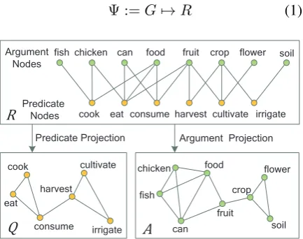
Figure 1: Illustration of (R) the bipartite graph of the verb-dobj-noun relation, (Q) the

predicate-projection monopartite graph, and (A)

the argument-projection monopartite graph.

Monopartite Graph Projection: In order to conduct random walk on the graph, we project the bipartite graph R onto a monopartite graph Q=(X, E) between the predicates, or A=(Y, E)

between the arguments (Zhou et al., 2007). Fig-ure 1 illustrates the intuition of the projection. The links inQrepresent the indirect connects between

the predicates inR. Two predicates are connected

inQif they share at least one common neighbor

argument inR. The weight of the links inQcould

be set by arbitrary distance measures. We referD

as an instance of the projectionQby a given dis-tance functionΦ.

Φ :=R_7→D (2)

Stochastic Walking Strategy: We introduce a

probability function∆to transform the predicate

distancesDinto transition probabilitiesP. Where P is a stochastic matrix, with each element pij

represents the transition probability from predicate

qi to qj. Generally speaking, nearby predicates

gain higher probabilities to be visited, while dis-tant predicates will be penalized.

Follow Equation 4, we aggregate over all orders of the transition probabilities P as the final

sta-tionary probabilitiesPe. According to the

Perron-Frobeniustheory, one can verify that it converges to dP(I −dP)−1 when P is non-negative and

regular matrix (Li et al., 2009). Where t

repre-sents the orders: the length of the path between two nodes in terms of edges. The damp factor

d_∈(0,1), and its value mainly depends on the

da-ta sparsity level. Typicallydprefers small values

such as0.005. It means higher order transitions

are much less reliable than lower orders (Liben-Nowell and Kleinberg, 2007).

e

P =

∞

∑

t=1

(dP)t

|(dP)t_|=dP(I−dP)−

1 ₍₄₎

Preference Propagation: in Equation 5, we combine the converged transition probabilities Pe with the measured preferences R as the propa-gation function: 1) for a given predicate, firstly it transfers to all nearby predicates with designed probabilities; 2) then it sums over the arguments preferred by these predicates with quantified s-cores to get smoothedRe. We further describe it-s configuration detailit-s in Section 4.4 and Equa-tion 12 with two propagaEqua-tion modes.

e

R=Pe∗R (5)

4 Model Configurations

4.1 Preference Ranking: Measure the Selectional Preferences

In collaborative filtering, usually there are explic-it and scaled user ratings on their item prefer-ences. For instance, a user ratings a movie with a score∈[0,10] on IMDB site. But in SP, the

pref-erences between the predicates and arguments are implicit: their co-occurrence counts follow the power law distribution and vary greatly.

Therefore, we employ a ranking function Ψto

measure the SP of the seen predicate-argument pairs. We suppose this could bring at least two benefits: 1) a proper measure on the preferences can make the discovering of nearby predicates with similar preferences to be more accurate; 2) while propagation, we propagate the scored pref-erences, rather than the raw counts or condition-al probabilities, which could be more proper and agree with the nature of SP smooth. We denote SelPref(q, a)as Pr(q, a)for short.

SelP ref(q, a) = Ψ(q, a) (6)

Previous literatures have well studied on various smooth models for SP. However, they vary great-ly on the measure of preferences. It is still not clear how to do this best. Lapata et al. investigate the correlations between the co-occurrence counts (CT)c(q, a), or smoothed counts with the human

plausibility judgements (Lapata et al., 1999; Lap-ata et al., 2001). Some introduce conditional prob-ability (CP)p(a_|q)for the decision of preference

judgements (Chambers and Jurafsky, 2010; Erk et al., 2010; S´eaghdha, 2010). Meanwhile, the point-wise mutual information (MI) is also employed by many researchers to filter out incorrect infer-ences (Pantel et al., 2007; Bergsma et al., 2008).

Ψ_CT =c(q, a) Ψ_{M I} =log p(q, a) p(q)p(a)

Ψ_CP = c(q, a)

c(q,_∗) ΨT D =c(q, a)log( m

|a_|)

(7)

In this paper, we present an adjusted ranking function (AR) in Equation 8 to measure the SP of seen predicate-argument pairs. Intuitively, it mea-sures the preferences by combining both the pop-ularity and association, with parameters control the uncertainty of the trade-off between the two. We define the popularity as the joint probability

p(q, a)based on MLE, and the association as MI.

This is potentially similar to the process of human plausibility judgements. One may judge the plau-sibility of a predicate-argument collocation from two sides: 1) if it has enough evidences and com-monly to be seen; 2) if it has strong association according to the cognition based on kinds of back-ground knowledge. This metric is also similar to the TF-IDF (TD) used in information retrieval.

Ψ_AR(q, a) =p(q, a)α1

(

p(q, a)

p(q)p(a)

)α₂

s.t. α1, α2 ∈[0,1]

(8)

We verify if a metric is better by two tasks: 1) how well it correlates with human plausibility judgements; 2) how well it helps with the smooth inference to disambiguate plausible and implausi-ble instances. We conduct empirical experiments on these issues in Section 5.3 and Section 5.4.

4.2 Distance Function: Projection of the Monopartite Graph

In Equation 9, the distance function Φis used to

discover nearby predicates with distance dij. It

guides the walker to transfer between predicates. We calculateΦbased on the vectorsqi, ⃗⃗ qj

repre-sented by the measured preferences inR.

dij = Φ(q⃗i, ⃗qj) (9)

WhereΦcan be distance functions such as Eu-clidean (norm) distance or Kullback-Leibler diver-gence (KL) etc., or oneminusthe similarity func-tions such as Jaccard and Cosine etc. The selection of distributional functions has been fully studied by previous work (Lee, 1999; Erk et al., 2010). In this paper, we do not focus on this issue due to page limits. We simply use theCosinefunction:

Φ_cosine(q⃗i, ⃗qj) = 1− ⃗ qi·q⃗j

∥qi⃗∥∥qj⃗∥ (10) 4.3 Probability Function: the Walk Strategy

We define the probability function ∆ as

Equa-tion 11. Where the transiEqua-tion probabilityp(qj|qi)

in P is defined as a function of the distance dij

with a parameterδ. Intuitively, it means in a given

walk step, a predicateqj which is far away from qi will get much less probability to be visited, and qi has high probabilities to start walk from itself

and its nearby predicates to pursue good precision. Once we get the transition matrixP, we can

com-putePeaccording to Equation 4.

p(qj|qi) = ∆(dij) =

(1₋dij)δ Z(qi)

s.t. δ_≥0, dij ∈[0,1]

(11)

Where the parameterδis used to control the

bal-ance of nearby and distant predicates.Z(qi)is the

normalize factor. Typically, δ around 2 can pro-duce good enough results in most cases. We verify the settings ofδin section 5.3.2.

4.4 Propagation Function

The propagation function in Equation 5 is repre-sented by the matrix form. It can be expanded and rewritten as Equation 12. Where pe(qj|qi) is the

converged transition probability from predicateqi

to qj. Pr(ak, qj) is the measured preference of

predicateqj with argumentak.

f

Pr(ak, qi) = m

∑

j=1

e

p(qj|qi)·Pr(ak, qj) (12)

We employ two propagation modes (PropMode) for the preference propagation function. One is

’CP’ mode. In this mode, we always set Pr(q, a)

as the conditional probabilityp(a|q)for the

prop-agation function, despite what Ψ is used for the

distance function. This mode is similar to previ-ous methods (Dagan et al., 1999; Keller and Lap-ata, 2003; Bergsma et al., 2008). The other is ’PP’ mode. We set ranking functionΨ=Pr(q, a)always

to be the same in both the distance function and the propagation function. That means what we propa-gated is the designed and scored preferences. This could be more proper and agree with the nature of SP smooth. We show the improvement of this extension in section 5.3.1.

5 Experiments

5.1 Data Set

Generalization Data: We parsed the Agence France-Presse (AFP) and New York Times (NYT) sections of the LDC English Gigaword corpo-ra (Parker et al., 2011), each from year 2001-2010. The parser is provided by the Stanford CoreNLP package1_{. We filter out all tokens containing} non-alphabetic characters, collect the <verb-dobj-noun>triples from the syntactically analyzed

da-ta. Predicates (verbs) whose frequency lower than

30 and arguments (noun headwords) whose

fre-quency less than5are excluded out. No other

fil-ters have been done. The resulting data consist of:

• AFP: 26,118,892 verb-dobj-noun

observa-tions with1,918,275distinct triples, totally

4,771predicates and44,777arguments.

• NYT: 29,149,574 verb-dobj-noun

observa-tions with3,281,391distinct triples, totally 5,782predicates and57,480arguments.

Test Data: For pseudo-disambiguation, we em-ploy Penn TreeBank-3 (PTB) as the test data (Mar-cus et al., 1999)2_{. We collect the 36,400} manu-ally annotatedverb-dobj-noundependencies (with

23,553distinct ones) from PTB. We keep depen-dencies whose predicates and arguments are seen in the generalization data. We randomly selec-t20% of these dependencies as the test set. We split the test set equally into two parts: one as the

developmentset and the other as thefinaltest set.

Human Plausibility Judgements Data: We employ two human plausibility judgements data

1_{http://nlp.stanford.edu/software/corenlp.shtml}

2_{PTB includes2,499stories from the Wall Street Journal}

for the correlation evaluation. In each they col-lect a set of predicate-argument pairs, and anno-tate with two kinds of human ratings: one for an argument takes the role as thepatient of a predi-cate, and the other for the argument as theagent. The rating values are between1 and7: e.g. they

assignhunter-subj-shootwith a rating6.9but2.8

forshoot-dobj-hunter.

• PBP: Pad´o et al. (2007) develop a set of hu-man plausibility ratings on the basis of the Penn TreeBank and FrameNet respectively. We refer PBP as their 212 patient ratings

from the Penn TreeBank.

• MRP: This data are originally contributed by McRae et al. (1998). We use all their 723

patient-nnratings.

Without explicit explanation, we remove all the selected PTB tests and human plausibility pairs from AFP and NYT to treat them unseen.

5.2 Comparison Methods

Since RSP falls into the unsupervised distribu-tional approach, we compare it with previous similarity-based methods and unsupervised gener-ative topic model3_.

Erk et al. (Erk, 2007; Erk et al., 2010) are the pioneers to address SP using similarity-based method. For a given(q, a)in relationr, the

mod-el sums over the similarities between a and the

seen headwords a′ ∈ Seen(q, r). They

investi-gated several similarity functionssim(a, a′)such

as Jaccard, Cosine, Lin, and nGCM etc., and dif-ferent weighting functionswtq,r(a′).

S(q, r, a) =∑

a′

wtq,r(a′) Zq,r ·

sim(a, a′) (13)

For comparison, we suppose the primary cor-pus and generalization corcor-pus in their model to be the same. We set the similarity function of their model as nGCM, use both the FREQ and DISCR weighting functions. The vector space is in SYN-PRIMARY setting with2,000basis elements.

Dagan et al. (1999) propose state-of-the-art similarity based model for word co-occurrence probabilities. Though it is not intended for SP, but it can be interpreted and rewritten for SP as:

Pr(a_|q) = ∑

q′_∈Simset(q)

sim(q, q′)

Z(q) p(a|q

′_{) (14)}

3_{The implementation of RSP and listed previous methods}

are available at https://github.com/ZhenhuaTian/RSP

They use the k-closest nearbys as Simset(q), with a parameter β to revise the similarity

func-tion. For comparison, we use the Jensen-Shannon divergence (Lin, 1991) which shows the best per-formance in their work assim(q, q′), and optimize

the settings ofkandβin our experiments.

LDA-SP: Another kind of sophisticated unsu-pervised approaches for SP are latent variable models based on Latent Dirichlet Allocation (L-DA). ´O S´eaghdha (2010) applies topic models for the SP induction with three variations: LDA, Rooth-LDA, and Dual-LDA; Ritter et al. (2010) focus on inferring latent topics and their distribu-tions over multiple arguments and reladistribu-tions (e.g., the subject and direct object of a verb).

In this work, we compare with ´O S´eaghdha’s original LDA approach to SP. We use the Mat-lab Topic Modeling Toolbox4 _{for the inference} of latent topics. The hyper parameters are set as suggestedα=50/T andβ=200/n, whereT is the

number of topics and n is the number of argu-ments. We testT=100,200,300, each with1,000

iterations of Gibbs sampling.

5.3 Pseudo-Disambiguation

Pseudo-disambiguation has been used for SP e-valuation by many researchers (Rooth et al., 1999; Erk, 2007; Bergsma et al., 2008; Chambers and Jurafsky, 2010; Ritter et al., 2010). First the sys-tem removes a portion of seen predicate-argument pairs from the generalization data to treat them as unseen positive tests (q, a+). Then it introduces

confounder selection to create a pseudo negative test (q, a−) for each positive (q, a+). Finally it

evaluates a SP model by how well the model dis-ambiguates these positive and negative tests.

Confounder Selection: for a given(q, a+_{), the}

system selects an argumenta′ from the

argumen-t vocabulary. Then by ensure(q, a′) isunseen in

the generalization data, it treatsa′ as pseudo a−.

This process guarantees that(q, a−)to be negative

in real case with very high probability. Previous work have made advances on confounder selec-tion with random, bucket and nearest confounder-s. Random confounder (RND) most closes to the realistic case; While nearest confounder (NER) is reproducible and it avoids frequency bias (Cham-bers and Jurafsky, 2010).

In this work, we employ both RND and NER confounders: 1) for RND, we randomly select

confounders according to the occurrence probabil-ity of arguments. We sample confounders on both the development and final test data with100

itera-tions. 2) for NER, firstly we sort the arguments by their frequency. Then we select the nearest con-founders with two iterations. One iteration selects the confounder whose frequency is more than or equal toa+, and the other iteration with frequency

lower than or equal toa+.

Evaluation Metric: we evaluate performance on both thepairwiseandpointwisesettings:

1) On pairwise setting, we combine correspond-ing(q, a+, a−)together as test instances. The

per-formance is evaluated based on the accuracy (AC-C) metric. It computes the portion of test instances

(q, a+, a−) which correctly predicted by the

s-mooth model with score(q, a+) > score(q, a−).

We weight each instance equally formacroACC, and weight each by the frequency of the positive pair(q, a+)formicroACC.

2) On pointwise setting, we use each positive test (q, a+) or negative test (q, a−) as test

in-stances independently. We treat it as a binary classification task, and evaluate using the standard area-under-the-curve (AUC) metric. This metric is firstly employed for the SP evaluation by Ritter et al (2010). FormacroAUC, we weight each in-stance equally; formicroAUC, we weight each by its argument frequency (Bergsma et al., 2008).

Parameters Tuning: The parameters are tuned on the PTB development set, using AFP as the generalization data. We report the overall perfor-mance on thefinal test set. While using NYT as the generalization data, we hold the same parame-ter settings as AFP to ensure the results are robust. Note that indeed the parameter settings would vary among different generalization and test data.

5.3.1 Verify Ranking Function and Propagation Method

This experiment is conducted on the PTB

devel-opment set with RND confounders. We use AFP

and NYT as the generalization data. For compari-son, we set the distance functionΦasCosine, with

defaultd=0.005, andδ=1.

In Table 1, the evaluation metric is Accuracy. The first 4 rows are the results of ’CP’ PropMode, and the latter 3 rows are the ’PP’ PropMode. With respect to the ranking function Ψ, CP performs

the worst as it considers only the popularity rather than association. The heavy bias on frequent pred-icates and arguments has two major drawbacks: a)

The computation of predicate distances would re-ly much more on frequent arguments, rather than those arguments they preferred; b) While propaga-tion, it may bias more on frequent arguments, too. Even these frequent arguments are less preferred and not proper to be propagated.

Crit. _{macro micro macro micro}AFP NYT

Ψ_CP 71.7 76.7 78.2 81.2 Ψ_{M I} 70.9 75.8 79.1 81.8 Ψ_{T D} 73.4 78.2 80.9 83.4 Ψ_AR 72.9 77.8 81.0 83.5 Ψ_{M I} 76.8 80.6 81.9 83.8 Ψ_{T D} 74.4 79.1 81.8 84.2

Ψ_AR 82.5 85.2 87.7 88.6

Table 1: Comparing different ranking functions.

For MI, it biases infrequent arguments with strong association, without regarding to the popu-lar arguments with more evidences. Furthermore, the generalization data is automatically parsed and kind of noisy, especially on infrequent predicates and arguments. The noises could yield unreliable estimations and decrease the performance. For T-D, it outperforms MI method on ’CP’ PropMode, but it not always outperforms MI on ’PP’ Prop-Mode. It is no surprise to find out the adjusted ranking AR achieves better results on both AFP and NYT data, withα1=0.2andα2=0.6. Finally,

it shows the ’PP’ mode, which propagating the de-signed preference scores, gains significantly better performance as discussed in Section 4.4.

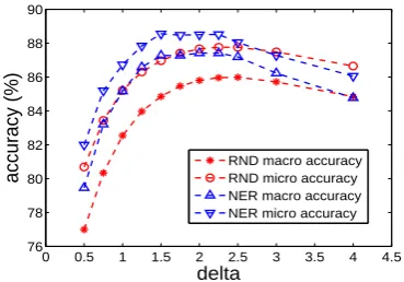
5.3.2 Verifyδof the Probability Function

This experiment is conducted on the PTB develop-menttests with both RND and NER confounders. The generalization data is AFP.

0 0.5 1 1.5 2 2.5 3 3.5 4 4.5 76

78 80 82 84 86 88 90

accuracy (%)

delta

RND macro accuracy RND micro accuracy NER macro accuracy NER micro accuracy

Criterion RND AFP NER RND NYT NER macro micro macro micro macro micro macro micro Erk et al.F REQ 73.7 73.6 73.9 73.6 68.3 68.4 63.8 63.0

Erk et al.DISCR 76.0 78.3 79.1 78.1 83.3 84.2 82.4 82.6

Dagan et al. 80.6 82.8 84.7 85.0 87.0 87.6 86.9 87.3

LDA-SP 82.0 83.5 83.7 82.9 89.1 89.0 87.9 87.8

RSPnaive 72.6 76.4 79.4 81.1 78.5 80.4 74.8 78.0

+Rank 74.0 77.7 83.5 85.2 81.4 83.1 84.5 86.9

+Rank+P P 83.5 85.2 87.2 87.0 88.2 88.2 88.0 88.3

+Rank+P P+Delta 86.2 87.3 88.4 88.1 90.6 90.1 91.1 89.3

Table 2: Pseudo-disambiguation results of different smooth models. Macro and micro Accuracy.

0 0.2 0.4 0.6 0.8 1

0 0.2 0.4 0.6 0.8 1

False Positive (FP)

True Positive (TP)

Erk et al. macroAUC=0.72 Dagan et al. macroAUC=0.80 LDA−SP macroAUC=0.77 RSP−ALL macroAUC=0.84

0 0.2 0.4 0.6 0.8 1

0 0.2 0.4 0.6 0.8 1

False Positive (FP)

True Positive (TP)

Erk et al. microAUC=0.62 Dagan et al. microAUC=0.83 LDA−SP microAUC=0.73 RSP−ALL microAUC=0.89

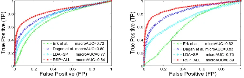
Figure 3: Marco and micro ROC curves of different smooth models.

We set the ranking function Ψ as AR (with

tuned α1=0.2and α2=0.6), the distance function

ΦasCosine, defaultd=0.005, and we restrictδ _∈

[0.5,4]. Figure 2 shows δ has significant impact

on the performance. Starting fromδ=0.5, the

sys-tem gains better performance while δ increasing.

It achieves good results around δ=2. This

mean-s for a given predicate, the penalty on itmean-s dimean-stant predicates helps to get more accurate smooth. The performance will drop ifδbecomes too big. This

means closest predicates are useful for smooth. It it not better to penalize them heavily.

5.3.3 Overall Performance

Finally we compare the overall performance of d-ifferent models. We report the results on the PTB

finaltest set, with RND and NER confounders. Table 2 shows the overall performance on Accu-racy metric. Among previous methods in the first 4 rows, LDA-SP performs the best in most cas-es. In the last 4 rows, RSPnaive means both the

ranking function and PropMode are set as ’CP’ and δ=1. This configuration yields poor

perfor-mance. Iteratively, by employing the adjusted

ranking function, smoothing with preference prop-agation method, and revising the probability func-tion with the parameter δ, RSP outperforms all

previous methods. The parameter settings of RSP-All areα1=0.2, α2=0.6, δ=1.75andd=0.005.

Figure 3 show the macro (left) and micro (right) receiver-operating-characteristic (ROC) curves of different models, using AFP as the generalization data and RND confounders. For each kind of previous methods, we show the best AUC they achieved. RASP-All still performs the best on the terms of AUC metric, achieving macroAUC at84% and microAUC at89%. We also verified

the AUC metric using NYT as the generalization data. The results are similar to the AFP data. It is also interesting to find out that the ACC met-ric is not always bring into correspondence with the AUC metric. The difference mainly raise on the pointwise and pairwise test settings of pseudo-disambiguation.

5.4 Human Plausibility Judgements

func-Criterion Spearman’s ρAFP Kendall’s τ Spearman’s ρNYT Kendall’s τ

PBP MRP PBP MRP PBP MRP PBP MRP

CT 0.49 0.36 0.37 0.28 0.54 0.44 0.41 0.34

CP 0.47 0.39 0.35 0.30 0.51 0.48 0.39 0.37

MI 0.56 0.39 0.43 0.31 0.54 0.49 0.41 0.38

TD 0.53 0.36 0.39 0.28 0.56 0.45 0.42 0.34

AR 0.58 0.40 0.44 0.31 0.58 0.50 0.44 0.39

Erk et al.F REQ 0.30 0.08 0.22 0.06 0.25 0.09 0.18 0.06

Erk et al.DISCR 0.06 0.21 0.04 0.15 0.16 0.23 0.11 0.16

Dagan et al. 0.32 0.24 0.24 0.18 0.46 0.29 0.34 0.21

LDA-SP 0.31 0.32 0.23 0.23 0.38 0.38 0.28 0.28

LDA-SP+Bayes 0.39 0.25 0.30 0.18 0.40 0.32 0.30 0.23

RSP-All 0.46 0.31 0.34 0.23 0.53 0.38 0.40 0.28

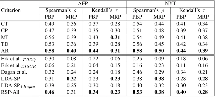
Table 3: Correlation results on the human plausibility judgements data.

tions and human ratings. Follow Lapata et al. (2001), we first collect the co-occurrence counts of predicate-argument pairs in the human plausibility data from AFP and NYT (before re-moving them as unseen pairs). Then we score them with different ranking functions (described in Section 4.1) based on MLE. Inspired by Erk et al. (2010), we do not suppose linear correlations between the estimated scores and human ratings. We use the Spearman’s ρ and Kendal’s τ rank

correlationcoefficient.

We also compare the correlations between the

smoothed scores of different models with human ratings. With respect to upper bounds, Pad´o et al. (2007) suggest that the typical agreement of human participants is around a correlation of0.7

on their plausibility data. We hold that automatic models of plausibility can not be expected to sur-pass this upper bound.

In Table 3, all coefficients are verified at signif-icant levelp<0.01. The first 5 rows are the

corre-lations between the preference ranking function-s and human ratingfunction-s bafunction-sed on MLE. On both the PBP and MRP data, the proposed AR metric better correlates with human ratings than others, withα2

>0.5andα1around[0.2,0.35]. The latter 6 rows

are the results of smooth models. It shows LDA-SP performs good correlation with human ratings, where LDA-SP+Bayes refers to the Bayes

predic-tion method of Ritter et al. (2010). RSP model gains the best correlation on the two plausibility data in most cases, where the parameter settings are the same as pseudo-disambiguation.

6 Conclusions and Future Work

In this work we present an random walk approach to SP. Experiments show it is efficient and effec-tive to address data sparsity for SP. It is also flex-ible to be applied to new data. We find out that a proper measure on SP between the predicates and arguments is important for SP. It helps with the discovering of nearby predicates and it makes the preference propagation to be more accurate. An-other issue is that it is not good enough to direct-ly applies the similarity or distance functions for smooth. Potential future work including but not limited to follows: investigate argument-oriented and personalized random walk, extend the model in heterogenous network with multiple link types, discover soft clusters using random walk for se-mantic induction, and combine it with discrimina-tive learning approach etc.

Acknowledgments

References

Eneko Agirre and David Martinez. 2001. Learning class-to-class selectional preferences. In Proceed-ings of the 2001 workshop on Computational Natu-ral Language Learning.

Shane Bergsma, Dekang Lin, and Randy Goebel. 2008. Discriminative learning of selectional pref-erence from unlabeled text. InEMNLP.

Carsten Brockmann and Mirella Lapata. 2003. Evalu-ating and combining approaches to selectional pref-erence acquisition. InEACL.

Nathanael Chambers and Dan Jurafsky. 2010. Improv-ing the use of pseudo-words for evaluatImprov-ing selection-al preferences. InACL.

Massimiliano Ciaramita and Mark Johnson. 2000. Ex-plaining away ambiguity: Learning verb selectional preference with bayesian networks. InCOLING.

Stephen Clark and David J. Weir. 2002. Class-based probability estimation using a semantic hierarchy. Computational Linguistics, 28(2):187–206.

Ido Dagan, Lillian Lee, and Fernando C. N. Pereira. 1999. Similarity-Based Models of Word Cooccur-rence Probabilities. Machine Learning, 34:43–69.

Katrin Erk, Sebastian Pad´o, and Ulrike Pad´o. 2010. A flexible, corpus-driven model of regular and inverse selectional preferences. Computational Linguistics, 36(4):723–763.

Katrin Erk. 2007. A simple, similarity-based model for selectional preferences. InACL.

Daniel Gildea and Daniel Jurafsky. 2002. Automatic labeling of semantic roles. Computational Linguis-tics, 28(3):245–288.

Jerrold J. Katz and Jerry A. Fodor. 1963. The structure of a semantic theory. Language, 39(2):170–210.

Frank Keller and Mirella Lapata. 2003. Using the web to obtain frequencies for unseen bigrams. Computa-tional Linguistics, 29(3):459–484.

Maria Lapata, Scott McDonald, and Frank Keller. 1999. Determinants of adjective-noun plausibility. In EACL, pages 30–36. Association for Computa-tional Linguistics.

Maria Lapata, Frank Keller, and Scott McDonald. 2001. Evaluating smoothing algorithms against plausibility judgements. In ACL, pages 354–361. Association for Computational Linguistics.

Lillian Lee. 1999. Measures of distributional similar-ity. In ACL, pages 25–32, Stroudsburg, PA, USA. Association for Computational Linguistics.

Hang Li and Naoki Abe. 1998. Generalizing case frames using a thesaurus and the mdl principle. Computational linguistics, 24(2):217–244.

Ming Li, Benjamin M Dias, Ian Jarman, Wael El-Deredy, and Paulo JG Lisboa. 2009. Grocery shop-ping recommendations based on basket-sensitive random walk. In SIGKDD, pages 1215–1224. ACM.

David Liben-Nowell and Jon Kleinberg. 2007. The link-prediction problem for social networks. Jour-nal of the American society for information science and technology, 58(7):1019–1031.

Jianhua Lin. 1991. Divergence measures based on the shannon entropy. IEEE Transactions on Information Theory, 37(1):145–151.

Mitchell P. Marcus, Beatrice Santorini, Mary Ann Marcinkiewicz, and Ann Taylor. 1999. Treebank-3.

Diana McCarthy, Sriram Venkatapathy, and Aravind K. Joshi. 2007. Detecting compositionality of verb-object combinations using selectional preferences. InEMNLP-CoNLL.

Ken McRae, Michael J. Spivey-Knowltonb, and Michael K. Tanenhausc. 1998. Modeling the influ-ence of thematic fit (and other constraints) in on-line sentence comprehension. Journal of Memory and Language, 38(3):283–312.

Sebastian Pad´o, Ulrike Pad´o, and Katrin Erk. 2007. Flexible, corpus-based modelling of human plausi-bility judgements. InEMNLP/CoNLL, volume 7. Patrick Pantel, Rahul Bhagat, Bonaventura Coppola,

Timothy Chklovski, and Eduard Hovy. 2007. Is-p: Learning inferential selectional preferences. In NAACL-HLT.

Robert Parker, David Graff, Junbo Kong, Ke Chen, and Kazuaki Maeda. 2011. English gigaword fifth edi-tion.

Philip Resnik. 1993. Selection and information: a class-based approach to lexical relationships. IRCS Technical Reports Series.

Philip Resnik. 1996. Selectional constraints: An information-theoretic model and its computational realization.Cognition, 61(1):127–159.

Philip Resnik. 1997. Selectional preference and sense disambiguation. InProceedings of the ACL SIGLEX Workshop on Tagging Text with Lexical Semantics: Why, What, and How. Washington, DC.

Alan Ritter, Mausam, and Oren Etzioni. 2010. A la-tent dirichlet allocation method for selectional pref-erences. InACL.

Mats Rooth, Stefan Riezler, Detlef Prescher, Glenn Carroll, and Franz Beil. 1999. Inducing a semanti-cally annotated lexicon via em-based clustering. In ACL.

Irena Spasi´c and Sophia Ananiadou. 2004. Us-ing automatically learnt verb selectional preferences for classification of biomedical terms. Journal of Biomedical Informatics, 37(6):483–497.

Kristina Toutanova, Christopher D. Manning, Dan Flickinger, and Stephan Oepen. 2005. Stochas-tic hpsg parse disambiguation using the redwood-s corpuredwood-s. Research on Language & Computation, 3(1):83–105.

Yorick Wilks. 1973. Preference semantics. Technical report, DTIC Document.

Hilmi Yildirim and Mukkai S. Krishnamoorthy. 2008. A random walk method for alleviating the sparsity problem in collaborative filtering. InProceedings of the 2008 ACM conference on Recommender system-s, pages 131–138. ACM.