Modelling the Electricity and Natural Gas Sectors for the Future Grid: Developing Co Optimisation Platforms for Market Redesign

Munich Personal RePEc Archive

Modelling the Electricity and Natural

Gas Sectors for the Future Grid:

Developing Co-Optimisation Platforms

for Market Redesign

Foster, John and Wagner, Liam and Liebman, Ariel

University of Queensland, Griffith University, Monash University

1 December 2015

Online at

https://mpra.ub.uni-muenchen.de/70114/

1

Modelling the Electricity and Natural Gas Sectors for the Future Grid:

Developing Co-Optimisation Platforms for Market Redesign

By

Prof John Foster,

Dr Liam Wagner,

Dr Ariel Liebman

Deliverables 4 and 5

:

CSIRO Future Grid Flagship Cluster

Project 3:Economic and investment models for future grids

2

Table of Contents

1 Introduction ... 5

2 Co-optimisation and Expansion of transmission networks and electricity generation for the Future Grid .... 6

2.1 Collaboration with Projects 1 and 2 ... 9

3 Electricity Market Simulation Platform. ... 10

3.1 Optimal Power Flow Solution ... 11

3.2 LT Plan ... 12

3.3 PASA... 13

3.4 MT Schedule ... 13

3.5 ST Schedule and Spot Market Dispatch ... 14

3.6 Short Run Marginal Cost Recovery Algorithm ... 16

3.7 Long Run Marginal Cost Recovery ... 16

3.8 Data and assumptions ... 17

3.8.1 Generation capacity and investment ... 17

3.8.2 Fuel Prices ... 18

3.8.3 Network ... 18

4 Natural Gas Market Modelling ... 19

4.1 Data ... 22

4.1.1 Natural Gas Demand ... 30

4.2 Base Case Simulation Results ... 33

5 Future Grid Scenario Modelling ... 36

5.1 The four influences ... 37

5.2 Scenario Kernels ... 38

5.3 Scenario Planning: BAU/Counter Factual ... 40

5.4 Scenario Correspondence between CFGF and the Project 3 CFGC ... 43

5.5 Representing the Scenarios for the CSIRO Future Grid Cluster ... 44

5.6 Scenario 1: “Set and Forget” ... 47

5.6.1 Assumptions and Data for Scenario 1 ... 48

5.6.2 Fuel Price Projections ... 50

5.6.3 Demand Projections ... 51

5.7 Initial Modelling Results ... 59

5.7.1 Wholesale market spot prices ... 59

5.7.2 Generation Profile ... 60

5.7.3 Concluding remarks ... 64

3

List of Figures

Figure 1: PLEXOS Simulation Core... 11

Figure 2: PLEXOS Least Cost Expansion Modelling Framework ... 13

Figure 3: World Gas Production Optimistic Case ... 20

Figure 4: The effects of international market linkage ... 21

Figure 5: Australia’s natural gas basins. Source: Geoscience Australia ... 24

Figure 6: Marginal Cost Curve for the Eastern Australian Gas Market ... 27

Figure 7: Sensitivity of the Golombek marginal cost of supply curve ... 28

Figure 8: Cooper Eromanga/Golombek marginal cost of supply curve ... 28

Figure 9: Stylized Network Diagram of the Eastern Australian Natural Gas Market ... 32

Figure 10: Marginal cost curve shift associated with a delay supply ... 34

Figure 11: Natural Gas Spot Prices Base Case Scenario ... 35

Figure 12: Supply node production schedule over time ... 35

Figure 13: Future Grid Forum core scenarios [78] ... 36

Figure 14: Projected Coal Prices (Medium Forecast) ... 50

Figure 15: NEM Demand Projections for Scenario 1 ... 51

Figure 16: Technology Costs for Conventional Electricity Generation ... 58

Figure 17: Technology Costs for Renewable Electricity Generation ... 58

Figure 18: Yearlywholesale electricity market spot prices (Load Weighted Average) ... 60

Figure 19: Installed Capacity by technology type for Scenario 1 ... 61

Figure 20: Generation profile by technology type for Scenario 1 ... 62

Figure 21: Installed Generation Capacity with respect to technological share ... 63

Figure 22: Generation Dispatch Quantities with respect to Conventional and Renewable Technologies ... 63

4

List of Tables

Table 1: Natural Gas Reserves within the Eastern States... 25

Table 2: Natural gas reserves by resource type ... 25

Table 3: Field reserve and production cost data example ... 26

Table 4: Golomobek Function Coefficients for Example Fields ... 29

Table 5: Main Transmission Pipelines ... 30

Table 6: Kernel elements ... 39

Table 7: BAU/Counter Factual Scenario Assumptions ... 41

Table 8: BAU/Counter Factual Scenario Kernels ... 42

Table 9: Project 3 and CSIRO Future Grid Forum Scenarios ... 45

Table 10: CFGF Scenarios and drivers ... 46

Table 11: CSIRO Future Grid Forum and the Cluster Project 3 Scenario drivers ... 47

Table 12: Mapping of the CSIRO Future Grid Forum “Set and Forget” Scenario to Project 3 Scenario Framework ... 52

Table 13: Representation of the CSIRO Future Grid Forum Scenario 1 Domestic Policy ... 53

Table 14: Representation of the CSIRO Future Grid Forum Scenario 1 International Forces ... 54

Table 15: Representation of the CSIRO Future Grid Forum Scenario 1 Demand Side Forces ... 55

Table 16: Representation of the CSIRO Future Grid Forum Scenario 1 Technological Development ... 56

5

1

Introduction

This report provides detail on the modelling and scenario frameworks for the economic

analysis of the Future Grid. These frameworks and modelling platforms have been

constructed to support the Future Grid Cluster in examining policy and market issues which

will affect the electricity and natural gas markets in Australia.

Initially we provide an overview of the co-optimisation and expansion of transmission

networks and electricity generation for the future grid. In this section we outline not only the

key mechanisms and analyses required, but also how we have and will continue to

collaborate with the other projects within the Future Grid Cluster.

In section 3 we provide an extensive analysis of the electricity market modelling platform

PLEXOS. This section will outline, not only the mechanistic components of modelling

electricity markets, but also some of the assumptions which are required to examine issues

such as generation investment under uncertainty.

The following section is a discussion of the natural gas modelling platform ATESHGAH.

This model has been in construction for several years prior to the commencement of the

Future Grid Cluster and represents a significant shift in gas market modelling methodology

for Australia, compared to previous approaches. This model is capable of examining multiple

issues associated with policy, market, economic, and physical aspects of gas production,

transmission, sale and liquefied natural gas (LNG) export simultaneously. We have used this

model to examine how Australia’s eastern gas market could be affected by the

commencement of LNG exports from Curtis Island in 2015/16.

In the remaining section, we present the scenario modelling framework as an overview and

present some initial results for Scenario 1: Set and Forget. These results represent the first set

of simulations and should thus be viewed as an initial attempt to undertake the large search

6

2

Co-optimisation and Expansion of transmission networks and

electricity generation for the Future Grid

The expansion of energy systems and its planning aims to address the problem of expanding

and augmenting electricity and natural gas infrastructure, while serving growing demand and

fulfilling a variety of technical, economic and policy constraints. Previously, the majority of

the energy system had been characterised by vertical integration, which allowed for the

optimal least-cost expansion subject to reliability and system constraints.

Since the implementation of market liberalisation [1-3], and the deregulation of the previous

vertically integrated supply chain into a number of horizontal components [4], there have

been a number of conflicting planning objectives which include:

1. The promotion of competition amongst electricity market participants by the

implementation of an aggregated spot market pool [5, 6]:

 The maximization of social welfare now occurs in a market based environment (i.e. the pool based market mechanisms [7, 8] and bilateral

contracts)

 Market participants can hedge risk via forward contract markets (contracts for

difference) which lower the probability of wholesale energy price spikes

affecting consumers [9]

 These market features provide non-discriminatory access to the lowest cost generation sources for all consumers connected to the main grid [10].

2. Facilitation of the early adoption of more efficient and lower cost generation

technology types [11]:

 Enhances the proliferation of generation assets which have a higher level of operational flexibility [12]

 The development of advanced technology such as Ultra-Super Critical Coal fired power stations [13].

3. Promoting the deployment and integration of renewable energy sources such as wind

and solar [14], which will lead to:

7  Diversification of fuel sources [16, 17].

4. Encouraging demand side participation via:

 Demand side management (DSM) [18, 19]

 Distributed Generation (DG) [20]

 Localisation of Storage [21, 22].

5. Constructing a robust and resilient physical electricity network which can adapt to and

enable processes which will:

 Ensure that the occurrence of network congestion remains low [23, 24]

 Reduce transmission losses

 Provide fair and adequate supply-side and demand-side reserves for all economic agents in the system (for supply-side agents [25, 26] and demand-side agents [27,

28])

 Promote resilience to uncertainties such as weather-related extreme events [29]

 Fairly price consumer security of supply requirements based on actual risks [30], rather than via fault-tolerant risk criterion values [31].

The deregulation and vertical restructuring of the power sector may lead to a significant

increase in the uncertainties and risk that central planner’s face when trying to maintain

adequacy of the energy system. Furthermore, this increase in risk and uncertainty may

decrease the potential options available to policy makers [32]. We now briefly outline the

uncertainties for power system planning in the future grid, which can be categorised into two

main elements:

1. Random uncertainties [33]

 Demand (load)

 Generation costs

 Bidding behaviour of generating units

 Availability of transmission capacity

 Generation asset availability

 Production from renewable energy sources. 2. Non-random uncertainties [34-36]

8  Load expansion and removal

 Transmission network augmentation

 Market rules and regulatory processes

 Fuel costs and availability

 Inflation or interest rates

 Environmental regulation

 Public Perception

 The dynamics of other energy and financial markets.

This project utilizing its gas and electricity market modelling platforms (outlined in Sections

3 and 4) has the capability to examine gas scheduling and its influence on outputs of both the

gas and power sectors. Furthermore, this combined modelling approach has the potential to

integrate gas market operations into system adequacy questions which relate to power system

reliability.

This project however, will not examine the effects of contracts, be they short- or long-term on

the natural gas market. It is likely that long-term contracts will be priced at the expected

value of long-term production costs with an added risk premium. However, we briefly

mention how our analysis could take into account gas market contracts and operations.

Medium- to long-term gas market scheduling is executed somewhat in accordance with gas

supply contracts.

In general terms, there are usually four types of gas supply contracts which warrant

discussion: long-term contracts; fixed delivery of volume and timing; flexible delivery of

volume and timing, and; the Take-or-Pay (ToP) contract arrangement. While supplementary

to bilateral over-the-counter arrangements, transactions on the gas spot market are mainly to

offset quantity deviations [37] and provide market liquidity and an indexed price for

long-term contracts.

To remain competitive, the majority of Open Cycle Gas Turbines (OCGT) require the use of

the more flexible and ToP type gas contracts. This reflects the price of these contract types

are typically below the other contract types previously mentioned. Thus, a consequence of

these types of contracting is that during periods of gas market infrastructure and supply

9

Furthermore, from a market operations perspective, non-electricity/LNG based consumers

(such as residential customers) should have a higher positioning on the schedule for dispatch.

This project has the capability to examine the prospect of insufficient gas supplies and how

this may compromise the power outputs of GPG units which may jeopardize the reliability of

the power system. Thus, gas transmission limits should also be taken into account when

examining the electricity generation capacity of GPG units as well as the possible shifts in

gas supply due to system curtailment and gas system operations.

In collaboration with the Universities of Newcastle and Sydney, our co-planning objective is

to maximize the overall social welfare function of consumers and to minimize total network

expansion and generation capacity costs.

In collaboration with Projects 1 and 2, our goal is to establish an integrated natural gas and

electricity market suite of constraints to understand system operational limits. The

fundamental constraints are transmission and supply constraints that involve the

combinations of generation/production, demand and line/pipeline flow. The transmission

constraints refer to technical limits for both gas pipelines and power lines. The supply

constraints refer to both gas production fields and power generators.

2.1 Collaboration with Projects 1 and 2

There are two ways in which Project 3’s database can be used: 1) some scenarios proposed by

P3 will be incorporated into P1 and P2 models, such as carbon prices, renewable energy

certificate prices forecast, fuel prices, etc. ;2) the gas price forecast, which can be considered

as gas production costs by basin/node. Next, a central gas dispatch scheme is performed

based on those costs of gas providers. Then we simulate gas prices in spot markets (bidding

to provide gas) to better inform the cluster of prevailing fuel price conditions. More

specifically, gas prices in Project 3's models will be gas production costs in models of P2.

This is due to the modelling platforms design purpose which is to provide gas prices from P2

models which are simulation results/outputs, reflecting gas demands as well as the market

10

3

Electricity Market Simulation Platform.

Modelling the National Electricity Market (NEM) has been conducted using a commercially

available electricity market simulation platform known as PLEXOS [38] provided by Energy

Exemplar. The core implementation of optimisation algorithms which drive this software

platform are primarily Linear Programming (LP), Non-Linear Programming (NLP), Mixed

Integer Programming (MIP), Quadratic Programming (QP), and Quadratic Constraint

Programming (QCP). Furthermore, the platform requires a number ofthird party industrial

solvers such as Gurobi, CPLEX and MOSEK to perform the transmission and generation

expansion planning.

PLEXOS utilizes these solvers in combination with an extensive input database of regional

demand forecasts, transmission thermal line limits and generation plant specifications to

produce price, generator behavioural characteristics (bidding behaviour) and demand

forecasts to replicate the NEM dispatch engine (NEMDE, formerly SPD (scheduling, pricing

and dispatch)) which is used by the Australian Energy Market Operator (AEMO) to operate

the market.

PLEXOS is a mature, and well respected modelling package and which is currently in use in

similar modelling-related research, including modelling the impact of electric vehicles on

Ireland’s electricity market [39, 40]. Furthermore, PLEXOS can provide a highly accurate prediction of prices and has been used to model market behaviour following the introduction

of carbon prices [41].

PLEXOS’ least cost expansion algorithm and planning tools, as used in this study and by AEMO [42], provides the optimal generation capacity mix given the current and forecasted

policy constraints [12, 43, 44].

Project 3 has specifically chosen PLEXOS as the key modelling platform for the Future Grid

Cluster given our previous research in modelling the future electricity grid and the

competitiveness of Australia’s electricity sector [45-47], and the platform is populated with

Australia’s NEM data [42, 48, 49] to enable robust modelling of the NEM.

In this project report, we now provide a short overview of the methodologies that PLEXOS

uses to simulate the electricity market and to evaluate its optimal expansion. The reader

should note however, the full description of the algorithmic development and methods that

11

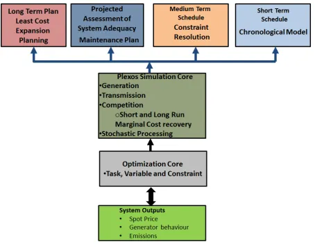
PLEXOS breaks down the simulation of the NEM into a number of phases which range in

scope and scale. These time-scales range from: year-long generation expansion planning and

constraint evaluation; security and systematic supply requirements; network expansion down

to hourly dispatch and market clearing. Although PLEXOS has the capability to perform

five-minute dispatch we will follow the method used by the Future Grid Forum [50] and

AEMO’s National Transmission and Network Development Plan [42], which both use hourly dispatch periods. This particular time scale is most useful in simulating long-term

electricity market structural behaviour patterns and in an effort to reduce the computational

requirements of this study. The operation and the interaction between these modelling phases

is shown in Figure 1. We shall now explore briefly the operational aspects of PLEXOS and the methodologies it employs to simulate the electricity market.

Figure 1: PLEXOS Simulation Core

3.1 Optimal Power Flow Solution

The solution to the optimal power flow (OPF), is one of the core functions of the PLEXOS

simulation engine which utilizes a linearized version of the direct current (DC) approximation

12

losses. In PLEXOS the locational marginal prices (LMP) are reflective of transmission

marginal loss factors as well as congestion throughout the system. Further, the congestion

modelling results are also an indicator of long-term constrains within sub-branch loops (such

as the Tarong loop in Queensland), which may require capacity upgrades in the future.

However, PLEXOS does not perform any pre-computation or impose any restrictions on how

dynamic the network data may be, thus it can model transmission augmentations and

transmission outages dynamically. PLEXOS thus optimizes the power flows using a

linearized DC approximation to the AC power flow equations. This model is completely

integrated into the mathematical programming framework that results in the realistic

simulation of generator dispatch, transmission power flows and regional reference pricing

which are jointly optimized with the power flow solution.

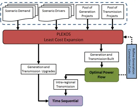
3.2 LT Plan

The long-term (LT) planning phase of the PLEXOS model establishes the optimal

combination of new entrant generation plant, economic retirements, and transmission

upgrades which will minimize the net present value (NPV) of the total costs of the system

over the planning horizon (as detailed in Figure 2). The following types of

expansions/retirements and other planning features are supported within the LT Plan:

 Building new generation assets (including multi-stage projects)

 Retiring existing generation plant

 Upgrading the capacity of existing transmission lines

 New build transmission line infrastructure (including multi-stage projects).

Furthermore, the PLEXOS least cost expansion planning phase also allows the tactful

inclusion of global and domestic policy drivers into its input data set. While the scenario

development capability of PLEXOS is an important issue into its operation, the

13

Figure 2: PLEXOS Least Cost Expansion Modelling Framework

3.3 PASA

The Projected Assessment of System Adequacy (PASA) schedules maintenance events such

that the optimal generation capacity is available and distributed suitably across

interconnected regions. The PASA phase of the model allocates/samples discrete and

distributed maintenance timings and random forced outage patterns for generators and

transmission lines. This ability to sample forced and planned outage patterns allows for

uncertainty in generation plant availability and informs the LT Plan expansion phase of the

model of further capacity requirements.

3.4 MT Schedule

The Medium Term (MT) Schedule is a model based on Load Duration Curves (LDC) (also

known as load blocks), that can run on daily, weekly or monthly resolutions which includes a

full representation of the power system and major constraint equations, but without the

complexity of individual unit commitment. The MT Schedule models constraint equations

14

 Fuel off-take commitments (i.e. gas take-or-pay contracts)

 Energy limits

 Long term storage management taking into account inflow uncertainty

 Emissions abatement pathways.

Each constraint is optimized over its original timeframe and the MT to ST Schedule’s bridge

algorithm converts the solution obtained (e.g. a storage trajectory) to targets or allocations for

use in the shorter step of the ST Schedule. The LDC blocks are designed with more detailed

information concerning peak and off-peak load times and less on average load conditions,

thus preserving some of the original volatility.

The solver/s used by PLEXOS will then schedule generation to meet the load and clear offers

and bids inside these discrete blocks. System constraints are then applied, except those that

define unit commitment and other inter-temporal constraints that imply a chronological

relationship between LDC block intervals. The LDC component of the MT Schedule

maintains consistency of inter-regional load profiles which ensures the coincident peaks

within the simulation timeframe are captured. This method is able to simulate over long time

horizons and large systems in a very short time frame. Its forecast can be used as a

stand-alone result or as the input to the full chronological simulation ST Schedule.

3.5 ST Schedule and Spot Market Dispatch

The Short Term (ST) Schedule is a fully featured, chronological unit commitment model,

which solves the actual market interval time steps and is based on mixed inter programming.

The ST Schedule generally executes in daily steps and receives information from the MT

Schedule which allows PLEXOS to correctly handle long run constraints over this shorter

time frame.

PLEXOS models the electricity market central dispatch and pricing for each state on the

NEM via Regional Reference Nodes (RRN). This is achieved by determining which power

stations are to be included for each dispatch interval in order to satisfy forecasted demand.

To adequately supply consumer demand, PLEXOS examines which generators are currently

bid into the market as being available to generate for the market at that interval. This

15

generators in the dispatch set in the given trading interval, taking into account the physical

transmission network losses and constraints can serve load.

Each day consists of 24 hour trading periods, and market scheduled generation assets have

the option to make a supply offer for a given volume (MW) of electricity at a specified price

($/MWh) across 10 bid bands. Each band, consists of bid price/quantity pairs which are then

included into the nodal bid stack.

Following the assembly of the generator bid pairs for each bid band, the LP algorithm begins

with the least cost generator and stacks the generators in increasing order of their offer pairs

at the node, while taking into account the transmission losses. The LP algorithm then

dispatches generators/power stations in merit order, from the least cost to the highest cost

until it dispatches sufficient generation to supply the forecasted demand with respect to the

inter-regional losses. This methodology replicates not only the NEM dispatch process but is

similar in construction to the least cost “Dutch Auction” [51, 52].

The price of the marginal generating unit at each time interval determines the marginal price

of electricity at the RRN for that given trading period. It should also be noted that this

dispatch process and the ST Schedule have the following properties:

 The dispatch algorithm calculates separate dispatch and markets prices for each node

and then for the Regional Reference Price for each state of the NEM

 Generator offer pairs determine the merit order for dispatch which and are adjusted with respect to relevant marginal loss factors

 The market clearing price is the marginal price, not the average price of all dispatched

generation (as per the “Dutch Auction” market design [53, 54]).

 Price differences across regions are calculated using inter-regional loss factor equations as outlined by AEMO [42, 49].

PLEXOS can produce market forecasts, by taking advantage of one of the following three

generator bidding behavioural models for cost recovery and market behaviour methodologies:

 Short Run Marginal Cost Recovery (SRMC, also known as economic dispatch)

 User defined market bids for every plant in the system

16

3.6 Short Run Marginal Cost Recovery Algorithm

The core capability of any electricity market model is to perform the economic dispatch or

Short Run Marginal Cost (SRMC) recovery based simulations of generating units across a

network to meet demand at least cost. PLEXOS’ platform performs economic dispatch under

perfect competition where generators are assumed to bid faithfully their SRMC into the

market. While simulations such as these will never result in a price trace which would match

historical market data from an observed competitive market, they provide a lower bound

representative of a pure competitive market.

3.7 Long Run Marginal Cost Recovery

PLEXOS has implemented a heuristic Long Run Marginal Cost (LRMC) recovery algorithm

that develops a bidding strategy for each generating portfolio such that it can recover the

LRMC for all its power stations. This price modification is dynamic and designed to be

consistent with the goal of recovering fixed costs across an annual time period. The cost

recovery algorithm runs across each MT Scheduled time step. The key steps of this algorithm

are as follows:

1. The MT Schedule is run with ‘default’ pricing (i.e. SRMC offers for each generating

units)

2. For each firm (company), calculate total annual net profit and record the pool revenue

in each simulation block of the LDC

3. Notionally allocate any net loss to simulation periods using the profile of pool

revenue (i.e. periods with highest pool revenue are notionally allocated a higher share

of the annual company net loss)

4. Within each simulation block, calculate the premium that each generator inside each

firm should charge to recover the amount of loss allocated to that period and that firm

equal to the net loss allocation divided by the total generation in that period – which is

referred to as the ‘base premium’

5. Calculate the final premium charged by each generator in each firm as a function of

the base premium and a measure how close the generator is to the margin for pricing

(i.e. marginal or extra marginal generators charge the full premium, while

infra-marginal generators charge a reduced premium)

6. Re-run the MT Schedule dispatch and pricing with these new premium values

7. If the ST Schedule is also run, then the MT Schedule solution is used to apply

17

method is run at each step. Thus, the ST Schedule accounts for medium-term

profitability objectives while solving in short steps.

In using PLEXOS, this project has set the LRMC recovery algorithm to run three times for

each time step to produce price trace forecasts with sufficient volatility and shape as

recommended by the software’s vendor, Energy Exemplar. This will ensure that under normal demand conditions, generating units will bid effectively to replicate market conditions

as seen in the NEM. It should be noted that the actual dispatch algorithm in this process is

still an LP based protocol which is in contrast to other commercial tools that use much slower

heuristic rule based algorithms to solve for LRMC recovery.

3.8 Data and assumptions

At the time of initiating this modelling the only publicly available PLEXOS data set that is

available is AEMO’s NTNDP 2014 [42]. However, this database requires significant

upgrading/repurposing so the database developed for this project was developed using the

NTNDP dataset and other publicly available data. Prior to this project a former database to

the NTNDP was used to model wholesale market behaviour in other related research such as:

the deployment of plug-in hybrid electric vehicles [55], distributed generation [20] and the

competitiveness of renewables [46]. The data and assumptions used to populate the database

have been developed such that the completed database includes the following details:

 Capacity factors (%)

 Ramp rates (MW/min)

 Emissions intensity factors (kg-CO2/MWh)

 Fuel costs ($/GJ) for coal, oil, distillate and natural gas

 Gas transport costs ($/GJ), where Moomba used as the NEM reference price

 Variable and fixed operating and maintenance costs ($/MWh and $/MW/year respectively)

 Scheduled outage rates and probability of forced outage rates (% hours/year).

3.8.1 Generation capacity and investment

Historical generation plant behaviour was sourced from AEMO’s data server [56], with technical specifications for all current generation assets sourced from AEMO, ACIL, Worley

18

with long-term supply contracts which were likely to be in place from 2030 onwards.

Inclusion of the above data provided an accurate predictor of generation plant likely to be

economically and technically feasible [42, 48, 49, 56, 61-65] for operation in 2035.

3.8.2 Fuel Prices

The cost projections for coal for use in QLD, NSW and VIC power generation were sourced

from recent assessments on fuel prices by AEMO and others [42, 48, 49, 56-60, 63, 66, 67].

Furthermore, due to the lack of infrastructure to support international trade, coal prices for

power generation are projected to remain subdued and stable until 2050. Natural gas costs

and market conditions are the subject of another model which will be discussed in Section 4.

3.8.3 Network

The network topology used within the modelling framework was initially sourced from

AEMO’s NTNDP [42], with its corresponding constraints on inter-region transmission flow. Upgrades to the network for this paper were only assumed if they had been previously

announced or currently under consideration by the market operator AEMO or the Australian

Energy Regulator (AER). Furthermore, the optimal expansion of the transmission network

19

4

Natural Gas Market Modelling

Australia is in a key geographic and strategic position to supply a sizable proportion of the

Asia Pacific regions’ LNG demand, and potentially be one of the world’s largest suppliers

(see [68]). Current trends in the development of the natural gas industry, particularly in

Western Australia, have shown that the internationalization of prices can have a significant

impact on electricity prices [69], carbon emissions [45, 47, 70], and the availability of gas for

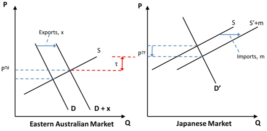
industrial users [71]. The effects of the expected uplift in prices with trade between two

markets, price in each adjusts depending on the elasticities of supply and demand (see Figure

4).

Further, the arbitrage opportunities which are presented to US produces to the detriment of

Australia’s interests are also of concern, such that the prevailing spot price in Japan has historically been much higher than the comparative European ports [72]. The newly

improved transport cost conditions (due to the upgrade of the Panama Canal) make East

Asian markets a very attractive prospect for US shale gas producers [73, 74].

While the demand for natural gas in Australia pales in comparison to its export potential [71],

there are numerous concerns surrounding the potential effects that exports may have on

industrial users and electricity generators. These competing interests are also apparent,

particularly between state governments, who are likely to receive a significant boost in

resource rents and somewhat higher availability of cheap supply for domestic consumption.

Aside from the significant coal reserves in Queensland, one of the key drivers for coal seam

gas exploration was the implementation of the Gas Electricity Scheme in 1994 [75, 76].

Accredited electricity generators could create tradable certificates which represented one

MWh of eligible generation. The schemes initial intention was to diversify the generation

mix, encouraging gas exploration and to offset the then high costs of using natural gas. This

inherent interest in using gas from electricity in Queensland was complemented by the

growing concern for reducing greenhouse gas emissions.

Similarly the New South Wales (NSW) government in 2003 implemented the NSW

Greenhouse Gas Abatement Scheme (NGGAS), which mandated a reduction in CO2

emissions per capita by 2007. The development of new gas powered generation assets which

20

capable of contributing to this abatement target. These two schemes were closed in 2013 and

2012 respectively due to the significant discovery of natural gas resources in QLD and the

introduction of national emissions reduction legislation [77].

21

Figure 4: The effects of international market linkage

The modelling framework ATESHGAH [78, 79], is well placed within the international

energy literature which has an extensive history of implementing Complementarity models

for examining oil and natural gas markets [80-82]. Many of these models that were

developed, address fundamental policy issues affecting natural gas markets. For example: the

disruption of Russian gas supplies via the Ukraine [83]; intra-European trade and capacity

bottlenecks [84, 85]; the potential cartelization of global gas markets [86]; the influence of

Eurasian gas supplies, and; the strategic implications of the South Stream pipeline [77]. The

use of Complementarity methods has also been used in a variety of studies which examine

the market liberalization process in a number of international contexts [87].

This report summarizes the inputs and overarching assumptions for the Non-Linear Program

(NLP) which in turn applies the Mixed Complementarity Problem (MCP) based framework,

to examine multi-producer oligopolistic agent behaviour via Nash-Cournot equilibrium in the

Eastern Australia natural gas market (EGM). This modelling platform has been developed in

GAMS to take advantage of its ability to model both economic problems, but also its

implementation of the MCP solver known as PATH [88-90]. More specifically, this

deterministic and myopic model examines the production trends, system adequacy and

22

The model developed by Wagner [78], is focused on analyzing the international linkages that

the EGM will have with its main export partners in Asia and the likely effects on production

and wholesale gas costs. The economic behaviour of agents in this newly minted

internationalized market is modelled via an optimization problem and market clearing

conditions. The principle agents which we have considered here are producers,

traders/marketers, and consumers in three crucial sectors (GPG, MMLI and LNG). The roles

of end-users and marketers have been simplified so that a producer who would normally face

several intermediaries before delivering to the final consumer, faces an aggregated demand

curve for each node in the network. In contrast to other models whose implementation of

multiple staged games [86] link several demand curves and a border price which would

overly complicate this model. We have assumed that producers act as semi-vertically

integrated agents whose roles fit more in context with the EGM [71, 78].

The primary objective for creating this model was to examine the strategic interactions

between the producer agents and LNG exporters. We have implicitly assumed that there is no

material benefit for disaggregating traders/marketers from the supply side. As noted above,

the aggregation of these roles is a reasonable and necessary assumption given that producers

such as Arrow and Origin not only sell at the bulk supply level, they consume natural gas as a

production input into markets such as GPG and LNG. Furthermore, as we only consider

yearly time intervals for demand we are able to avoid any issues with long-term contracts for

supply and spot market behavioural issues which is in keeping with the international

experience with modelling these types of markets [91-93] and more specifically their

linkage/interconnection [94].

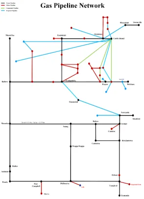
4.1 Data

The purpose of this model is to provide a comprehensive representation of all producers in

the EGM. The data set includes all producing fields (by owner/operator), pipelines

(transmission and major laterals) and demand by the three main gas consuming sectors within

23

We assume that there is an integrated producer/trader/marketer agent whose objective is to

maximize profits when faced with nodal inverse demand curves. The lack of data availability

on nodal Mass Market (MM) and Light Industrial (LI) demand (excluding utility gas powered

generation), is one of the limitations of this model. Aggregate historical and forecasts of

demand for the combined sector MM/LI is used to maintain the appropriate level of scope for

this analysis. Similar agent aggregations have also been seen in the international literature,

and the experience with modelling the European [83, 91, 93] and US markets [92], further

justifies our methodology.

Initially the base year 2013, is used to parametrize the model for simulation, which allows us

to establish the yearly and long-term structural consequences of international market linkage

for the EGM with its key Asian trading partners. The literature which examines similar

markets/regional trade blocks, has deemed it sufficient to evaluate these situations via yearly

time steps [86, 92, 95]. The omission of daily or seasonal effects associated with demand may

lead to different results, especially in the presence of binding transport constraints and high

levels of capacity utilization. However, the use of storage and inter-period arbitrage by

producers/processors can overcome some of these difficulties [92, 95].

The data and analysis presented in this report are represented in SI units. Therefore, reserves

are expressed in petajoules (PJ); production, transport capacity and demand in PJ/year, which

allows for us to neglect differential qualities and facilitate constraint qualifications to be

uniformly applied. We shall now explore the construction of the base case data set and detail

the possible scenarios and their implementation.

The availability of resources in the EGM has been sourced from the technical literature [83,

86], state and federal regulators [71, 96, 97], the market operator [98-100], industry analysts

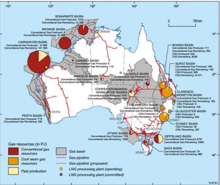
[66, 101-103] and corporate reporting [104, 105] (also see Figure 5). The discovery, firming

up and transformation of reserve tranches are all sourced and calculated exogenously to this

modelling framework [97, 102, 103]. The 13 basins’ reserve and resource base case data is

shown below in Table 1 and Table 2 (by basin and by resource type). It should be noted that

each basin is associated with a single resource type. For example, the resources associated

with Surat/Bowen are considered conventional natural gas, whereas the Bowen and Surat

24

Figure 5: Australia’s natural gas basins. Source: Geoscience Australia

Production costs have been sourced from a range of commercial services, industry reports

and government reports [71, 100]. Each field is composed of tenures and grouped by

geological formation and owner/developer (as in [106, 107]). Each field (producing area) has

detailed estimates of reserves and resources with a range of costs associated with extraction

(cf. [99]). The costs associated with each tranche of possible production is then used to

calibrate the supply cost curve (via the Golombek supply cost function [108]).

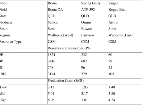
Table 3 shows example fields with corresponding reserves and costs. We also provide the

cumulative cost curve for natural gas by production tranche within each basin (see Figure 6).

It shows that 50% of all available reserves have an expected production cost of $5.16/GJ,

which far exceeds the expected average cost of US shale gas production at $2-3/GJ? [92,

25

Table 1: Natural Gas Reserves within the Eastern States

Basin Resource 2P 3P 2C 3C URR

Type (PJ) (PJ) (PJ) (PJ) (PJ)

Bass Conventional 338 250 360 268 726

Bowen CSG 8,535 25,130 4,345 2,834 31,488

Clarence/Moreton CSG 445 2,922 2,511 629 6,062

Cooper/Eromanga Mixed 2,198 1,901 6,416 244 8,488

Galilee CSG - - 259 1,634 1,634

Gippsland Conventional 3,890 3,859 1,094 10,000 14,192

Gloucester CSG 669 832 - - 832

Gunnedah CSG 1,426 1,426 3,460 - 4,886

Maryborough Shale - 3,000 - - 3,000

Otway Conventional 604 - 274 - 878

Surat CSG 28,835 38,831 11,979 - 50,810

Surat-Bowen Conventional 76 106 2,000 - 2,106

Sydney CSG 424 728 - - 728

Totals 47,440 78,985 32,698 15,609 125,830

Table 2: Natural gas reserves by resource type

Resource 2P 3P 2C 3C URR

Type (PJ) (PJ) (PJ) (PJ) (PJ)

Conventional 1,790 2,007 4,176 244 6,349

CSG 40,334 69,868 22,554 5,097 96,440

Offshore 4,832 4,109 1,728 10,268 15,796

Shale - 3,000 - - 3,000

Unconventional 5 - 4,240 - 4,245

26

Table 3: Field reserve and production cost data example

Node Roma Spring Gully Kogan

Field Roma OA ATP 592 Kogan East

State QLD QLD QLD

Producer Santos Origin Arrow

Basin Surat Bowen Surat

Region Walloons (West) Fairview Walloons (East)

Resource Type CSM CSM CSM

Reserves and Resources (PJ)

2P 1824 232 60

3P 2416 682 79

2C 758 96 25

URR 3174 779 105

Production Costs ($/GJ)

Low 3.13 1.93 1.40

Mid 5.04 3.17 3.80

High 6.06 3.81 4.24

27

Figure 6: Marginal Cost Curve for the Eastern Australian Gas Market

The functional form of the Golombek primary cost function

𝐶𝑖(𝑣𝑖) = 𝛼 ∗ 𝑣𝑖 +1_{2 𝛽 ∗ 𝑣}𝑖2− 𝛾 ∗ (𝑉𝑖 − 𝑣𝑖) ∗ ln (1 −𝑣_𝑉𝑖

𝑖) − 𝛾 ∗ 𝑣𝑖,

(1)

The marginal cost function is as follows:

where vi, is the volume of production in time t, α is the minimum cost of production, β and γ

are parameters fitted to the change in production costs associated with accessing increasingly

deeper and more difficult to extract gas and Vi is the remaining reserves. The sensitivity of

each of the aforementioned coefficient is presented in Figure 7. We present three key supply fields with their associated Golombek coefficients in Table 4 and an example of the marginal cost curve for the unconventional Cooper/Eromanga fields in Figure 7.

𝑀𝐶𝑖(𝑣𝑖) = 𝛼 + 𝛽 ∗ 𝑣𝑖− 𝛾 ∗ ln (1 −𝑣_𝑉𝑖 𝑖),

28

Figure 7: Sensitivity of the Golombek marginal cost of supply curve

29

Table 4: Golomobek Function Coefficients for Example Fields

Node Roma Spring Gully Kogan

Field Roma OA ATP 592 Kogan East

Α 3.35 4.70 3.01

Β 0.061 0.0044 0.00108

Γ -0.015 -0.00099 -0.003157

Processing capacity is sourced from AEMO’s annual planning reports (GSOO [99, 100]), and it should also be noted that processing capacity is dealt with implicitly as an exogenous upper

bound on production capacity. Thus, expansion timing and entry timing of processing plant is

derived from AEMO [100].

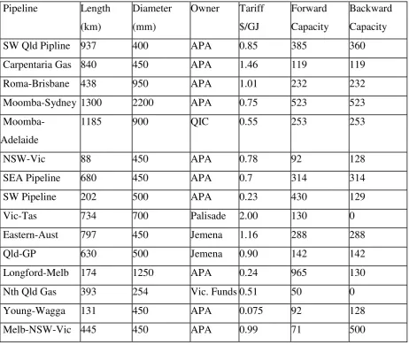
Transport pipelines and the formation of the network topology has been derived from [99,

100], and more generally from [101]. The maximum flow capacity along each pipeline

pathway within the network of nodes, is by necessity an exogenous input into the model.

Contrary to the production and processing capacities, the dual of the utilization in network

capacity is required for the model formation. Pipeline network expansion can also be

implemented via scenarios for policy planning and analysis or with optimal expansion

techniques discussed in André [110]. We present the main transmission pipelines which

30

Table 5: Main Transmission Pipelines

Pipeline Length Diameter Owner Tariff Forward Backward

(km) (mm) $/GJ Capacity Capacity

SW Qld Pipline 937 400 APA 0.85 385 360

Carpentaria Gas 840 450 APA 1.46 119 119

Roma-Brisbane 438 950 APA 1.01 232 232

Moomba-Sydney 1300 2200 APA 0.75 523 523

Moomba-Adelaide

1185 900 QIC 0.55 253 253

NSW-Vic 88 450 APA 0.78 92 128

SEA Pipeline 680 450 APA 0.7 314 314

SW Pipeline 202 500 APA 0.23 430 129

Vic-Tas 734 700 Palisade 2.00 130 0

Eastern-Aust 797 450 Jemena 1.16 288 288

Qld-GP 630 500 Jemena 0.90 142 142

Longford-Melb 174 1250 APA 0.24 965 130

Nth Qld Gas 393 254 Vic. Funds 0.51 50 0

Young-Wagga 131 450 APA 0.075 92 128

Melb-NSW-Vic 445 450 APA 0.99 71 500

4.1.1 Natural Gas Demand

The demand for natural gas by the LNG sector has been initially sourced from [71, 96, 100,

101, 103]. We assume that the required minimum capacity utilization rate for each of the

proposed liquification facilities is set at 93% [111]. Furthermore, the timing of demand is a

key variable, and is therefore considered in the scenario planning capability of this model. It

should be noted that the demand is assumed to incorporate the losses associated with pipeline

transport and liqification as is presented via the "as-produced" method in a similar fashion to

the electricity sector [112, 113]. The timing of additional liquification plant trains to

correspond to export demand, further developments in gas reserves and international demand,

31

The reference prices of demand for gas by the LNG sector is derived from the Free-on-board

(Fob) netback equivalent price with respect to the Japanese hub Cargo-insurance-freight price

(Cif). The derived Cif prices presented here for model calibration is sourced from the burner

tip equivalent of the Japanese Crude Cocktail (JCC) price for oil translated into a gas price

via the standard oil index linked S-curve [111, 113]. The demand curve, an iso-elastic

non-linear function is represented with respect to our assumptions of quantity and reference price

via the JCC/S-Curve pricing methodology [113].

The electricity generation sector is greatly affected by a shift in price and availability of

natural gas [47]. As such, the future development of Gas fired Power Generation (GPG) is

particularly sensitive to long-term prices and has had similar market integration issues when

gas supply networks have been interconnected via international exports (e.g. Western

Australia [111]). The demand for natural gas by GPG’s has been sourced from [100].

Furthermore, technical specifications for each of these power stations is sourced from [42, 48,

49, 57, 58, 62, 63, 112, 114]. We calibrate the likely bounds of demand given historical

operating capacities [42, 49], as a mid-point estimate. The upper and lower bounds for

natural gas demand is derived from each GPG’s installed capacity, heat rate (GJ/MWh), the

type of operation (baseload, intermediate or peaking) and the technology type of the gas

turbine (open or combined cycle), are all used to exogenously parameterize each power

station.

The combined Mass Market/Light Industry sector historical and forecasts of demand for

natural gas has been calculated from AEMO [100] and BREE [71, 96]. Historical prices at

each of the corresponding nodes to AEMO’s original network topology [99, 100] have been

used to parametrize the iso-elastic inverse demand curve for the sector. Elasticities of demand

have been sourced from the literature to further aid in the construction of this model [

115-118]. We have chosen to represent the demand for natural gas in any node/market m, by

applying a non-linear iso-elastic demand function which can be represented as follows:

𝐷𝑚 = 𝐷𝑚𝑂[𝑃𝑚_𝑃(𝐷𝑚) 𝑚𝑂 ]

𝜎𝑚

32

where 𝐷_𝑚 and 𝑃_𝑚(𝐷_𝑚) are the levels of demand and price at equilibrium, 𝐷_𝑚𝑂 and 𝑃_𝑚𝑂 are the

reference (historical) demand and prices respectively in market m in 2013 [98]. The price

elasticity of demand 𝜎_𝑚, for the three sectors in this model (GPG, LNG and MM/LI) is

sourced from previous literature [117, 119, 120]. As mentioned earlier in this report, we shall

neglect the full technical description of the market clearing conditions and algorithmic

methods for simulating this market model and again refer the reader to [78].

33 4.2 Base Case Simulation Results

The base case scenario presented here creates a comparative benchmark for future scenario

development for policy analysis. This base case is largely used as a mechanism for parameter

validation and as a proof of concept rather than a most likely case and should be viewed as

such. Initially, we assume that the Japanese Cif price remains high, which corresponds to the

medium scenario for global oil prices which reaches ~160/bbl in 2040 [121]. Demand for

natural gas has been derived from the AEMO Gas statement of Opportunities (see [99, 100]).

Electricity market generation behaviour has been derived from AEMO [42, 48, 49] and we

further assume that entry timing and retirements are within the bounds of previously reported

rates [47].

The LNG sector is assumed to have an investment and production profile that is largely

derived from [99, 100]. Furthermore, we also assume that the entry of ARROW gas reserves

will be delayed and the associated national supply and marginal cost curve is shifted to the

left (see Figure 10). While this shift in the supply curve is dramatic, the resulting gas prices for the Eastern Australian capital cities are still somewhat in line with the expectations of

AEMO and Core Energy’s analysis [102, 103]. While world gas markets are now in turmoil given the current Saudi Arabian led OPEC over production of oil and gas, the world being

awash with gas is still a somewhat interesting and important scenario to examine. The results

presented in Figure 11 and Figure 12, while not out of sample with AEMO [100], nor its counterpart Core Energy [103], estimate that prices will remain high. This base case

mentioned here represents a proof of concept for the modelling platform and its integration

34

Figure 10: Marginal cost curve shift associated with a delay supply

35

Figure 11: Natural Gas Spot Prices Base Case Scenario

36

5

Future Grid Scenario Modelling

In this section we will provide an overview of the scenario frameworks employed by Project

3 and the CSIRO Future Grid Cluster [50]. We will then provide a brief overview of the

relationships between the CSIRO’s Future Grid Forum (CFGF) Scenarios and how the cluster

will proceed with its modelling. Furthermore, this report will largely focus on Project 3’s

modelling results for the first of the CFGF scenarios with an expanded sensitivity and parameter suite.

Figure 13: Future Grid Forum core scenarios [50]

Project 3 will reexamine and re-establish the CFGF scenarios from first principles and this reformulation will allow for the Future Grid Cluster projects to take into account a broader

range of: policy/regulatory; economic/market and technological influences. These three key system influencer categories are inextricably linked and therefore need to be modelled.

Furthermore, these drivers are the cornerstone to scenario development and quite like a chain

37

Firstly, the key influencers were summarized into ten scenario kernel elements that are

somewhat independent of each other. We then generate a set of “Reduced Scenarios” that can be used for discussion, scenario selection and external communication purposes. Secondly,

scenarios are represented via all of their explicit sub-components which reflect the “micro”

inputs which generate the parameter suite that needs to be modelled explicitly.

5.1 The four influences

The four categories of key influences and their inter-relationships are set out in this Section

and we provide a further overview of Project 3’s scenario construction and integration with

the CFGF.

1) Policy (and regulatory) decisions

 Actions in the policy and regulation space which are under the control of Australian policymakers and stakeholders

 Policy actions are orthogonal to states of the world

 Can depend on outcomes of states of the world

 Policy and regulatory decisions can be classified into either supply- or demand-side focused.

2) States of the World

 Forces or influences that are outside Australia’s control are described here by the

following three categories:

a. Supply-side forces: These include changes in the parameters of key supply

side technologies, such as technology costs and costs of fuel feed-stocks

b. Demand-side forces, that are further divided into two sub-categories, those

being:

Structural and behavioural, and

Technological development related

c. International Forces which includes actions of markets and policy decisions by

other countries.

38

Many policy and states of the world need to be modelled as having two or three outcomes.

Some are binary (yes/no) and some are sensitivities with several states. We chose to limit

sensitivities to three levels, that is, low, medium, and high (or slow, medium, and fast in the case of rate based parameters, such as technological learning). This limitation is imposed in

order to limit the extent of the combinatorial explosion that arises when combining all the

different possible outcomes.

4) Linkages

There are also interactions between the various forces and their sensitivities. In particular, it

is important to note that there can be linkages within and between forces in the following two

categories:

 States of the world

 Policy.

5.2 Scenario Kernels

In order to facilitate the communication of Project 3’s modelling results for scenarios that are

relevant to policy and investment decisions, we need to work at an appropriate level of detail.

Since the Future Grid Cluster is only concerned with the impacts of policies and external

forces on large-scale infrastructure investments and wholesale market behaviour, the kernel

scenarios will be handled at this level. The structure for developing the Project 3 scenarios is

39

Table 6: Kernel elements

Kernel Element States of the World

Supply Side Low/Slow Medium High/Fast

Technology

costs and

selection

Fossil Technology

costs

1

Renewable/Zero

emission

Technology costs

reduction

2

Fossil Fuel Costs 3

Climate policy

Carbon Pricing 4

Renewable Energy

Target

5

Electricity

Demand

Decline BAU High

Energy Growth

(GWh)

6

Demand

profile changes

Decrease Status

Quo

Increase

Load Factor

Change

7

-> Day Status

Quo

-> Night

Day to Night

Load peak shift 8

Policy Support

for renewable

generation

Yes No

Transmission Super projects 9

Scale Efficient Network Extensions 10

The above table sets out the ten kernel elements grouped into three major categories: supply

40

three sensitivities and a further two which have two sensitivities. This leads to a total of

26,244 possible combinations which are not easily manageable for without a methodology

such as ours.

5.3 Scenario Planning: BAU/Counter Factual

Establishing a set of scenarios which examines the possible future given a set of prior

assumptions is a difficult exercise [122-124]. The most common starting point for any

investigation using the “Scenario Analysis” methodology [125, 126], is to create a counter-factual that may or may not represent our future expected states, but is used as a reference

state for comparison [127].

This counterfactual in our case is used to create a well-defined rule based environment whose

main value is to elucidate the current state of affairs in the electricity sector and to understand

an idealised representation completely [46, 128]. While a very idealised picture of the

electricity market may turn out to be an approximate and somewhat incomplete picture of the

real world, its “valuefulness” lies in the construction of such a conceptual framework [128], as outlined in this report and the previous deliverables [129, 130]. Furthermore, due to recent

policy volatility and an increasingly visible trend in the decline of electricity demand this

scenario shouldn’t be regarded as a “Business As Usual” case study. Furthermore, this methodology remains useful as a reference or counterfactual scenario against which other

scenarios could be compared [125, 128, 130-132].

While this BAU/Counter Factual is mostly self-explanatory the broad aspects of this scenario

are as follows:

 Demand for electricity is assumed to be increasing in terms of total annual energy (as generated) and with respect to peak demand.

 The shape of the load duration curve and load factors for each of the NEM states

remains the same (as shown in the 2012 and 2014 AEMO NTNDPs’ [42, 133]).

 Greenhouse gas (GHG) and Renewable Energy Target (RET) policies are both assumed to be with the moderate/medium carbon price trajectories and the previous

RET (41 TWh at 2020 which equates to roughly 20% of all electricity generated).

 Technological costs, for conventional (combustion) and renewable energy generators have been sourced from a survey of the best available forecasts (i.e. from [42, 45, 50,

41

The assumptions used to develop this BAU/Counter Factual scenario are presented in Table 7 and were originally developed for a similar exercise by this project team [45, 137]. Following the broad overview presented in Table 7 we will now provide the homoeomorphic mapping into the scenario kernel elements via

Table 8.

Table 7: BAU/Counter Factual Scenario Assumptions

Forces underpinning

scenario

Long-term historic trend consumption growth

No consumer reaction to rising prices

Gas prices reflect global energy trends

Climate change not an issue

No recognition of technology shift to renewables and

distributed generation

Capital costs (2035)

CCGT $1100/kW

OCGT $1100/kW

Wind $2558/kW

Network topology Existing

Generation locations Located close to transmission infrastructure

Modelling

assumptions Wind intermittent to 30% capacity factor

Fuel price

(Moomba), (2035)

Medium Gas $8.32/GJ

Low gas price $4.89/GJ

42

Table 8: BAU/Counter Factual Scenario Kernels BAU/ Counter Factual

Kernels

Kernel

Eleme

nt

States of the World

Supply Side Low/Slo

w Medium

High/Fas

t

Technology costs

and selection

Fossil Technology

costs 1 X

Renewable/Zero

emission

Technology costs

reduction

2 X

Fossil Fuel Costs 3 X

Climate policy

Carbon Pricing 4 X

Renewable Energy

Target 5 X

Electricity Demand Decline BAU High

Energy Growth

(GWh) 6 X

Demand profile

changes

Load Factor

Change

Decrease Status Quo Increase

7 X

Day to Night

demand peak shift

-> Day Status Quo -> Night

8 X

43

generation

Transmission Super projects 9 X

Scale Efficient Network Extensions 10 X

5.4 Scenario Correspondence between CFGF and the Project 3 CFGC

The CFGF has taken a similar and somewhat related approach to developing its own scenario

suite but has traversed a slight different path via its need to use detailed modelling levers.

This has translated into a modelling and simulation input based approach. Furthermore, the

scope and scale of the CFGF had the additional requirement of examining distribution system

investment due to expansion, asset replacement and end-user pricing impacts and for the

potential for changing elasticities in demand.

The CFGF scenarios have been constructed via three differentiators:

 Centralised generation versus distributed generation

 Significance of peak demand growth and the flattening (skewness) of the load profile

 Deployment of large scale renewable energy generation projects.

These differentiators are represented within this projects’ scenario modelling framework,

while also incorporating the relationships between the scenario Kernels (as illustrated in

Table 9). Furthermore, the CFGF scenario drivers are shown in Table 10 below.

Below in Table 9, the relationship between this projects methodology of using supply- and demand-side based drivers, and the CFGF scenarios is shown. Given that there are a variety

of ways that drivers can be classified, we have used a mapping matrix as a guide to

translating between the two slightly different approaches. As we have reported previously

[129, 130], for example, we break the growth of distributed generation (DG) impacts into

three components which then become drivers for the modelling scenarios: energy efficiency;

and load profile changes of two kinds, load factor changes; and shifts of the peak to different

times of the day. While this matrix is not exhaustive, experience is needed to transform the

input data into inputs using our framework. We have done this in Project 3 by setting up the