Munich Personal RePEc Archive
Boundedly Rational Expected Utility
Theory
Navarro-Martinez, Daniel and Loomes, Graham and Isoni,
Andrea and Butler, David and Alaoui, Larbi
Universitat Pompeu Fabra, Warwick Business School, Warwick
Business School, Mudoch University, Universitat Pompeu Fabra
15 June 2017
1
Boundedly Rational Expected Utility Theory
Daniel Navarro-Martinez
Department of Economics and Business, Pompeu Fabra University, and Barcelona Graduate School of
Economics, Ramon Trias Fargas 25-27, 08005 Barcelona, Spain.
Corresponding author. Tel.: +34 935421467. E-mail address: [email protected].
Graham Loomes
Warwick Business School, University of Warwick, Coventry CV4 7AL, UK.
Andrea Isoni
Warwick Business School, University of Warwick, Coventry CV4 7AL, UK.
David Butler
Murdoch School of Management and Governance, Murdoch University, Perth, Australia.
Larbi Alaoui
Department of Economics and Business, Pompeu Fabra University, and Barcelona Graduate School of
2
Boundedly Rational Expected Utility Theory
Abstract
We build a satisficing model of probabilistic choice under risk which embeds Expected Utility Theory
(EUT) into a boundedly rational deliberation process. The decision maker accumulates evidence for and
against alternative options by repeatedly sampling from her underlying set of EU preferences until the
evidence favouring one option satisfies her desired level of confidence. Notwithstanding its EUT core, the
model produces patterns of behaviour that violate standard axioms, while at the same time capturing the
systematic relationship between choice probabilities, response times and confidence judgments, which is
beyond the scope of theories that do not take deliberation into account. [92 words]
Keywords: Expected utility; bounded rationality; deliberation; probabilistic choice; confidence; response
times.
3
1. Introduction
Economics is often said to be the study of the allocation of scarce resources, of how human beings decide to
combine their time and skills with physical resources to produce, distribute and consume. However,
economic models may sometimes ignore the fact that arriving at decisions is itself an economic activity and
that the hardware and software involved – that is, the human brain and its mental processes – are themselves
subject to constraints. Herbert Simon emphasised this point in his 1978 Richard T. Ely lecture, in which he
discussed the implications of attention being a scarce resource.1 In a world where there are many (often complex) choices to be made, spending time on any one decision entails an opportunity cost in terms of the
potential fruits of other decisions that might have been considered instead. Being unable to devote unlimited
time and attention to every decision they encounter, humans generally have to satisfice rather than optimise.
Simon bemoaned the lack of interest among economists in the processes that individuals use when
deciding how to allocate their scarce mental resources, and he advocated “building a theory of procedural
rationality to complement existing theories of substantive rationality”. He suggested that “some elements of
such a theory can be borrowed from the neighboring disciplines of operations research, artificial
intelligence, and cognitive psychology”, but noted that “an enormous job remains to be done to extend this
work and to apply it to specifically economic problems” (Simon, 1978, pp.14–15).
Although there have been some developments along these lines (e.g., Gilboa and Schmeidler, 1995;
Rubinstein, 1998; Gigerenzer and Selten, 2001), the decades that followed Simon’s lecture saw the
mainstream modelling of individual decision making – especially with respect to choice under risk and
uncertainty – take a different direction. Stimulated by experimental data that appeared to violate basic
axioms of rational choice, a number of models appeared at the end of the 1970s and in the early 1980s that
sought to provide behavioural alternatives to standard Expected Utility Theory (EUT) – see Starmer (2000)
for a review. Typically, these were deterministic models that relaxed a particular axiom and/or incorporated
various additional features – e.g., reference points, loss aversion, probability weighting, regret,
disappointment – to try to account for certain regularities in observed decisions. While such models
provided more elaborate descriptive theories of choice, little or no consideration was given to the mental
constraints referred to by Simon. His invocation to build boundedly rational procedural models largely fell
by the wayside in the field of risky decision making.
Thus we now have an impressive array of alternative models, each of which can claim to
accommodate some (but not all) of the observed departures from EUT. However, being typically
deterministic and for the most part process-free, these models have no intrinsic explanation for at least three
other pervasive empirical regularities in the data, which may arise from features of the decision-making
1
4
process: first, the probabilistic nature of most people’s decisions;2 second, the systematic variability in the time it takes an individual to respond to different decision tasks of comparable complexity;3 and third, the degree of confidence decision makers (DMs) express about their decisions.4
So, in this paper, we propose to explore the direction Simon advocated and investigate the potential
for applying a boundedly rational deliberative process to the ‘industry standard’ model of decision making
under risk and uncertainty, EUT. We start by identifying in general terms what is required of a procedural
model of preferential choice. We then consider how the various components of such a model might be
specified in ways that are in keeping with conventional economic assumptions while at the same time
allowing for scarcity of time and attention. The resulting model – which we call Boundedly Rational
Expected Utility Theory (BREUT) – generates a number of implications, not just about choice probabilities,
but also about process measures such as response times and confidence in the decisions made. A striking
result is that, despite being based on EU preferences, the model produces choice patterns that deviate from
EUT in line with some well-known decision making phenomena, and we characterise the circumstances
under which this occurs.
We shall not claim that the particular mechanisms used in BREUT to model deliberation are a
literal representation of the way the mind actually operates. Psychology and neuroscience cannot yet tell us
precisely how the brain generates decisions, so BREUT is necessarily a stylisation intended to capture some
broad procedural features using conventional modelling elements. Also, while we take EUT as the ‘core’ of
our model, we wish to stress that we are not asserting that EUT is necessarily the correct account of the way
people’s underlying preferences are configured. As we shall explain in due course, our broad modelling
strategy has the potential to be extended to many non-EU core theories. This paper may be understood as a
‘proof of concept’ exercise: that is, an exploration of the implications of embedding EUT in a simple and
reasonable boundedly rational procedure for arriving at decisions.
In the next section, we present our instantiation of BREUT, focusing upon the kind of binary
choices between lotteries with monetary outcomes that have been the staple diet of many decision-making
experiments. In Section 3, we demonstrate how BREUT provides a parsimonious account of the systematic
relationship between choice probabilities, decision time and confidence. We show that the model entails
respect for first order stochastic dominance and weak stochastic transitivity but allows patterns of choice that
violate strong stochastic transitivity, independence and betweenness. In the final section, we consider the
2 When participants are presented with exactly the same decision task displayed in exactly the same way on two or
more separate occasions within the same experiment, they often give different responses on different occasions. See Mosteller and Nogee (1951) for an early example; Luce and Suppes (1965) for a review of the early theoretical literature; and Rieskamp et al. (2006), Bardsley et al. (2010, Chapter 7), and Baucells and Villasís (2010) for more recent discussions. The same pattern of variability has also been observed in more applied settings, such as the judgments of software developers or of medical doctors (see Kahneman et al., 2016).
3
See, for example, Tyebjee (1979), Birnbaum and Jou (1990), Busemeyer and Townsend (1993), Wilcox (1993), Moffatt (2005), Rubinstein (2007, 2013), Spiliopoulos and Ortmann (2016), Achtziger and Alós-Ferrer (2014).
5
relationship between our model and others in the psychology and economics literature. We discuss some
limitations of the model in its current form, together with what we see as the most promising directions for
extending our approach and some other possible implications of our findings. The Appendix reports the
proofs of our theorems.
2. The Model
The term ‘bounded rationality’ has been interpreted in somewhat different ways – see Munier et al. (1999)
and Harstad and Selten (2013) for examples – so it may be helpful to start by clarifying the way in which we
are using it.
Bounded rationality has often been characterised in terms of the difficulties DMs may encounter
when they are faced with complex problems or environments involving information that is hard to obtain
and process. However, we suggest that even in cases in which there are just two alternatives whose
properties are clearly specified, bounded rationality plays a role in terms of the deliberative process used by
a DM to arrive at a decision. Straightforward though a choice might appear, it will often still require some
thought to identify and evaluate the arguments pulling in opposing directions. Since a DM has many other
things to do in her lifetime, it is impossible to devote unlimited time and attention to any single decision.
Instead, she has to find a way to allocate her limited attention to the various decisions that she faces – which
is to say, she must have some mechanism to decide when to cease further deliberation, make a decision and
move on to the next task. It is the process underlying the allocation of time and attention between different
decisions that we regard as fundamental to the characterisation of bounded rationality.
Behavioural scientists have invested substantial effort in developing various approaches for
modelling decision-making processes: see, for example, elimination by aspects (Tversky, 1972); the
adaptive decision maker framework (Payne et al., 1993); the priority heuristic (Brandstätter et al., 2006); and
query theory (Johnson et al., 2007), to name only a few. Another influential stream of literature has
developed an accumulator or sequential-sampling framework (for reviews, see Ratcliff and Smith, 2004;
Otter et al., 2008). Most such accumulator models have been developed in the context of perceptual tasks
(e.g., judging the colour or comparative brightness of objects, or the relative numbers of dots in different
areas of a screen, or the relative lengths of lines, and so on). The application of these models to preferential
choice has been less common, although Busemeyer and Townsend’s (1993) Decision Field Theory (DFT)
and its extensions constitute a notable exception. We will discuss the relationship between BREUT and DFT
in more detail in Section 4.
The general idea behind such models is that a DM starts from a position where she does not already
have a decisive preference for any one of the available options and therefore has to acquire evidence that can
help to discriminate between them. In the case of preferential choice, this evidence comes from introspecting
about the relative (subjective) desirability of the possible consequences and the weights to be attached to
each of them. As evidence is accumulated, it is as if the DM continually re-assesses the relative strengths of
6
further sampling of evidence – that is, further deliberation – is required. However, once the judged relative
advantage of one option over the other(s) crosses some threshold, the process is terminated and the option
favoured by the accumulated evidence is chosen. The DM can then allocate her scarce attention to
something else.
Such models typically consist of three components:
(i) some representation of the sources of evidence from which samples are drawn – in this context,
the underlying stock of subjective values or judgments;
(ii) some account of the way the sampled evidence is accumulated;
(iii) a stopping rule which terminates the accumulation process and triggers a decision.
In the next three subsections, we explain how BREUT models these three components and we
describe the resulting behavioural variables.
2.1. The Structure of Underlying Subjective Values
Consider the following seemingly simple decision. A DM is asked to choose between lottery A, which
(omitting any currency symbol) offers the certainty of 30, and lottery B, which offers a 0.8 chance of 40 and
a 0.2 chance of 0. She might be told that the uncertainty will be resolved by drawing a ticket at random from
a bag containing 100 tickets numbered from 1 to 100 inclusive: if she chooses A she will get 30 whichever
ticket is drawn; if she chooses B she will receive 40 if the ticket is between 1 and 80 inclusive, while a ticket
between 81 and 100 gives 0.
Using standard EUT notation, with ≽ denoting weak preference, the decision can be written as:
𝐴 ≽ 𝐵
Û
𝑢(30) ≥ 0.8 𝑢(40) + 0.2 𝑢(0). (1)
Deterministic EUT supposes that it is as if each DM acts according to a single utility function that
gives an exact answer to this question (and gives the same answer every time that this question is asked).
But cognitive psychology and neuroscience suggest that there is no unique and instantly accessible
subjective value function – see, for example, Busemeyer and Townsend (1993), Gold and Shadlen (2007),
Stewart et al. (2006, 2015). Rather, a typical DM will have had many experiences and impressions of what
30 and 40 represent in subjective terms. So it may require some retrieval from memory and some reflection
to balance the arguments pulling in opposite directions. On the one hand, lottery B offers a 0.8 chance of a
higher payoff – 40 rather than 30; but A offers a 0.2 chance of getting 30 rather than 0. For a typical DM, it
may not be immediately obvious exactly where the subjective value of 30 is located in the range between the
subjective values of 0 and 40 nor precisely how the differences, weighted by the probabilities, balance out.
So arriving at a decision may involve deliberating about the balance of evidence obtained by sampling from
those experiences and judgments.
Since we are investigating the effects of embedding EUT in a boundedly rational deliberation
7
von Neumann-Morgenstern (vNM) utility functions, u(.), normalised so that u(0) = 0.5 At this point, we place no restrictions upon the nature of this distribution, although in Section 3 we make more specific
assumptions in order to explore the behaviour of the model and derive predictions for commonly used pairs
of lotteries.
The assumption of a distribution of vNM functions was made by Becker et al. (1963a) when they
proposed their “random utility model for wagers”, which has since come to be known as the random
preference (RP) model. This way of representing the variability from moment to moment of people’s states
of mind might be seen as an early example of a ‘multiple-selves’ modelling strategy that has been applied to
various areas of economic behaviour (e.g., Elster, 1987; Alós-Ferrer and Strack, 2014). The key difference
between the RP model and ours is that Becker et al. supposed that DMs only sampled once for each
decision, applying a single randomly-picked u(.) to both options, whereas we assume that deliberation
involves sampling multiple times, as we now describe.
2.2. Modelling the Sampling and Accumulation of Evidence
Adapting the general framework of accumulator models to the specific context of binary choice between
lotteries, in BREUT each sample is modelled as a random draw of a utility function from the core
distribution of u(.), which is applied to the pair of lotteries under consideration. Using probabilities as
weights, as EUT entails, this yields a subjective value difference which we denote by V(A, B) and which
takes some positive value when a u(.) is drawn that strictly favours A, takes a value of zero when the two
options are exactly balanced and takes a negative value when the sampled u(.) strictly favours B. We can
represent this difference as a difference between the monetary certainty equivalents (CEs) of the two
options. Formally, for any u(.) sampled,
𝑉 𝐴, 𝐵 = 𝐶𝐸5− 𝐶𝐸7 = 𝑢89(𝐸𝑈5) − 𝑢89(𝐸𝑈7). (2)
We use differences in CEs rather than in utilities because CEs are measures that can be legitimately
compared and aggregated across utility functions. It is well known in economics that comparisons of utilities
(or their aggregation) across different utility functions are not theoretically meaningful and lead to
problematic results. This is true even if utilities are normalized, for example to be between 0 – for the worst
possible outcome in a particular set – and 1 – for the best possible outcome (see Hammond, 1993; Binmore,
5 In EUT, as presented by von Neumann and Morgenstern (1947), the argument(s) of u(.) could be anything – money,
8
2009, for a detailed discussion of this topic). This argument is typically addressed to comparison or
aggregation of utilities across people, but the same logic holds for the case of having multiple utility
functions that represent different mental states within one person (as if there were multiple selves). There is
no basis for claiming that the difference between the best and the worst possible outcomes represents the
same amount of satisfaction in one mental state (or self) as in another one. For this reason, we need to put
V(A, B) in a ‘common currency’ that can be legitimately aggregated. The use of CEs is a straightforward
way of achieving that, which has a number of precedents in the literature (e.g., Luce, 1992; Luce et al.,
1993; Cerreia-Vioglio et al., 2015).
For each sampled u(.), the CE difference provides a signal not only about which option is better, but
also about how much better it is. Repeated sampling (with replacement) produces a series of realisations of
V(A, B), which are accumulated by progressively updating their mean and sample standard deviation,
denoted respectively by 𝑉(𝐴, 𝐵) and 𝑠<(5,7).
As noted at the end of Section 1, what we are proposing is a model, not a literal account of how the
human brain actually works. We are not suggesting that people really precisely calculate V(A, B) at every
moment. Rather, we are exploring a way of modelling aggregation of sampled differences which is
consonant with a deliberative process applied to an EUT core, and which could also be extended to other
core theories that researchers might wish to consider in future work, given that most decision theories entail
the existence of CE differences between pairs of alternatives.
This way of aggregating evidence has important implications. Let E[V(A, B)] denote the mean of the
distribution of CE differences for the pair of lotteries {A, B} implied by the individual’s underlying
population of u(.). If the individual takes a sample of size k from this distribution, that sample will have a
mean which we denote by 𝑉=(𝐴, 𝐵). Taking sufficiently many samples of size k will result in some
distribution for 𝑉=(𝐴, 𝐵). Independently of the value of k, this distribution will always have a mean equal to E[V(A, B)]. However, as implied by the central limit theorem, when k becomes larger, the distribution of
𝑉=(𝐴, 𝐵) will be increasingly similar to a normal distribution with a variance inversely related to k. If the
individual were to deliberate indefinitely – that is, if k were allowed to tend towards infinity – the variance
of the distribution of 𝑉=(𝐴, 𝐵) would tend towards zero and the whole distribution would collapse towards E[V(A, B)]. This straightforward implication of the central limit theorem will be particularly useful to shed
light on the operation of our model in the following sections. In essence, if an individual had unlimited time
to devote to any one decision, that would constitute a limiting case in which she would always arrive at the
same judgment about the sign and size of 𝑉(𝐴, 𝐵), as given by E[V(A, B)], with no variability. However, in reality, unlimited deliberation is infeasible, so the individual will need to decide when the accumulated
9
2.3. Modelling the Stopping Rule
In a number of models, including Busemeyer and Townsend’s (1993) DFT, the process of accumulating
evidence in a binary choice can be represented as a random walk or a diffusion process which terminates
when the path crosses a (typically fixed) threshold. However, it is often unclear what determines the position
of the thresholds, and it is not obvious that they should be fixed. On the one hand, for decisions in which
there is a lot at stake and for which there is considerable variance in the evidence, we might expect the
thresholds to be set a relatively long way from zero in order to avoid jumping too quickly to what might be
the ‘wrong’ choice. But until the DM has collected some evidence, she has little information about the
variance and therefore cannot set the initial threshold distance appropriately. On the other hand, if there is
actually little difference between the options, then having fixed parallel thresholds entails the possibility that
it could take an unrealistically long time to reach one or other threshold in cases in which the consequences
of picking the wrong option are negligible.
To address these issues, we propose an approach which, in effect, sets thresholds that are responsive
both to the evolving pattern of the evidence as it accumulates and to the DM’s wish to limit the time spent
deliberating about any particular decision. The key to our stopping rule is the DM’s desired level of
confidence: in particular, we propose that the DM deliberates until she concludes that the accumulated
evidence gives her sufficient confidence to make a choice. In BREUT, confidence is represented as the
probability that the DM picks the option that she would choose after unlimited deliberation – i.e., the option
implied by the sign of E[V(A, B)].6
We suggest that the notion of individuals attempting to achieve a personal desired level of
confidence is a simple and intuitive way of building a satisficing model, and also one for which there is
some empirical support (see Hausmann and Läge, 2008). In contrast with the optimal stopping tradition (see,
e.g., Stigler, 1961; Shiryaev, 1978), this approach does not require us to assume that the individual has
detailed knowledge about the opportunity cost of additional sampling in terms of forgone benefits from
potential future activities. We simply require that the DM can form an impression of the confidence level
she wants at the time the decision is made.7
We denote the DM’s desired level of confidence as Conf. Because deliberation is costly in terms of
the opportunity costs associated with each extra draw, we allow the DM to progressively reduce Conf as the
amount of sampling increases. The idea here is that the longer she spends trying to discriminate between
options, the more likely she is to conclude that there is not much between them, so that she has less to fear
from choosing the wrong option. Specifically, we assume that the desired level of confidence after k draws is
given by:
6
If E[V(A, B)] = 0, the DM is indifferent between A and B in the limit. We shall assume that, in such a case, she chooses each option with probability 0.5.
7 It will be clear from the following sections that our main choice results do not depend on the use of this particular
10
𝐶𝑜𝑛𝑓 = max [0.5, 1 − 𝑑 𝑘 − 1 ], (3)
where k≥ 2 and where d (with 0 < d≤ 0.5) is a parameter that captures the rate at which the DM reduces her
Conf as k increases, subject to the constraint that Conf≥ 0.5.
d may vary from one individual to another, reflecting different tastes for the trade-off between more
input into the current decision and turning attention to something else. A person with a very low d is
someone who wants to be very confident in her decisions, and therefore is willing to invest more time
deliberating. The limiting case is when d → 0, in which the individual wants to be absolutely sure of making
the right decision and deliberates indefinitely. On the other hand, someone with a high value of d is ready to
make decisions with less confidence and spends relatively less time deliberating. Thus when d has the
maximum value of0.5, the DM makes her decision after just two samples, choosing the option favoured by
the mean of the two sampled CE differences. Modelling d as a personal characteristic provides a degree of
within-person consistency with just one parameter. It would be possible to construct a more complicated
function for Conf, but the linear form in Expression 3 is sufficient for our ‘proof of concept’ purposes.8 We then model the DM’s decision about whether or not she should terminate her deliberation as if
she were applying a sequential t-test. Again, we acknowledge the as if nature of this assumption. Other ways
of modelling the stopping rule are possible, but a sequential statistical test meshes well with the idea of
achieving some personal level of confidence. What we try to capture is the idea that when the choice is
initially presented – i.e., before any deliberation has occurred – the DM starts with the null hypothesis that
there is no significant difference between the subjective values of the two options. However, as the evidence
accumulates, it is as if she continually updates 𝑉(𝐴, 𝐵) and 𝑠<(5,7) and combines them to form a test statistic
Tk:
𝑇= = < 5,7
KL(M,N) = . (4)
This statistic is then used to determine whether the null hypothesis of zero difference can be rejected at the
level of Conf corresponding to k. This occurs if the following condition is met:
𝐹=89[abs(𝑇=)] ≥ 𝐶𝑜𝑛𝑓, (5)
where Fk – 1[·] is the c.d.f. of the t-distribution with k ‒ 1 degrees of freedom. If the weak inequality in
Expression 5 is not satisfied, the DM is assumed to continue sampling and to continue reducing Conf until
the hypothesis of zero difference is rejected in favour of one of the alternatives – at which point, she chooses
whichever option is favoured according to the sign of 𝑉(𝐴, 𝐵). The value of k when sampling stops and a
8 For instance, one could allow the DM to reduce her desired level of confidence more slowly when the stakes are
11
choice is made is denoted by k*, the level of confidence at that point is Conf* and the value of the test
statistic at that point is Tk*.
2.4. Behavioural Variables Generated by BREUT
Because of its procedural nature, BREUT gives a richer description of decision making than process-free
models. The outcome of the deliberation process can be summarised by three main behavioural variables:
choice probabilities, confidence and response times. We now consider each of these in more detail.
2.4.1. Choice probabilities
In BREUT, the probability of choosing A over B, denoted by Pr(A
!
B), is the probability that the nullhypothesis is rejected with a positive Tk*. The complementary probability that B is chosen is the probability
that the null hypothesis is rejected with a negative Tk*.
In the classic RP model, it is as if an individual samples just once per decision and chooses on the
basis of the single u(.) sampled on that occasion. In that one-shot model, the probability of choosing A over
B is given by the proportion of utility functions that favour A over B in the underlying core distribution. We
denote this probability by Pr Core(A
!
B). However, BREUT supposes that an individual samples more thanonce, so that the effective Pr(A
!
B) will typically be different from Pr Core(A!
B). As noted in Section 2.2,the central limit theorem implies that the variance of the distribution of 𝑉=(𝐴, 𝐵) decreases as k becomes larger and the whole distribution gets more concentrated around E[V(A, B)]. As a consequence, as k
increases, the DM becomes increasingly likely to choose the option favoured by the sign of E[V(A, B)]. In
the limit, the probability of choosing A over B as k tends towards infinity, denoted by Pr Lim(A
!
B), is either0 (if E[V(A, B)] is negative) or 1 (if E[V(A, B)] is positive). This means that:
0 = Pr Lim(A
!
B) ≤ Pr(A!
B) ≤ Pr Core(A!
B) if E[V(A, B)] < 0(6) Pr Core(A
!
B) ≤ Pr(A!
B) ≤ Pr Lim(A!
B) = 1 if E[V(A, B)] > 0.That is, Pr(A
!
B) will always lie between the core probability in the one-shot RP model and the limitingprobability (0 or 1) implied by the sign of the mean of the distribution of CE differences.
Expression 6 has some important implications. First, if one of the lotteries is never favoured by the
individual’s core utility functions (i.e., Pr Core(A
!
B) is either 0 or 1), then there will be no amount ofsampling for which that lottery will be chosen with positive probability (i.e., it will always be the case that
Pr(A
!
B) = Pr Core(A!
B) = Pr Lim(A!
B)). Since dominated lotteries are never chosen in EUT, this entailsthat BREUT necessarily satisfies first-order stochastic dominance. Second, since (other things being equal)
lower values of d imply larger values of k*, Pr(A
!
B) will tend towards Pr Lim(A!
B) as d decreases: inother words, with more deliberation, choice probabilities become more extreme. Third, if Pr Lim(A
!
B) andPr Core(A
!
B) are on different sides of 0.5 for some core, then BREUT allows for one lottery to be the12
1 and 3 in Section 3 will show how this allows a stable core of vNM utility functions to produce Allais-type
violations of EUT’s independence axiom.
2.4.2. Confidence
In BREUT, the degree of confidence in a decision, Conf*, is the level of Conf used in the test that rejects the
null hypothesis and triggers a choice in favour of one of the alternatives after k* samples. The range of the
confidence measure is (0.5, 1) – see Expression 3.
While a substantial literature has investigated and modelled confidence judgments in decision tasks
that have a correct answer (see Pleskac and Busemeyer, 2010, and references therein), there are only a few
isolated exceptions of studies investigating confidence in preferential choice (e.g., Butler and Loomes, 1988;
Sieck and Yates, 1997). To the best of our knowledge, there are no other decision models that explicitly
address confidence in preferential decisions. However, confidence is clearly regarded as an important factor
in various areas of economics (e.g., Acemoglu and Scott, 1994; Ludvigson, 2004; Dominitz and Manski,
2004; Barsky and Sims, 2012) and it might be desirable if decision theories had more to say about this
dimension. A distinctive feature of BREUT is that its stopping rule automatically produces predictions about
the DM’s confidence in the decision made.9
2.4.3. Response time
Since deliberation is modelled through sequential sampling, BREUT can make predictions about the length
of time that it takes to make a decision – the response time (RT). It is reasonable to assume that RT is an
increasing function of the number of samples, k*, required to reject the null hypothesis. In addition, RT can
also be expected to be positively related to the complexity of the decision problem. As there is no generally
agreed index of complexity for such choices, for the purposes of this paper we make the simple assumption
that complexity is reflected by the total number of consequences (NC) appearing in any pair.10 This is a straightforward way of capturing the intuition that, if there are more items to consider, each deliberation step
will take longer. So we propose the following basic specification for RT:
𝑅𝑇 = 𝑘∗∙ 𝑁𝐶. (7)
Since k* is a stochastic variable, RT is also stochastic, implying that the DM is liable to take
different amounts of time to reach a decision for the same pair of alternatives on different occasions. Given
Expression 3 and the definition of k*, it follows that RT = [(1 – Conf*)/d + 1]NC. That is, RT and Conf* are
9
There may also be interesting questions to be asked about the effects on behaviour when DMs are prevented from achieving their desired level of confidence – for example, when operating under time constraints (e.g., Kocher et al., 2013) and having to make a choice before the null hypothesis can be rejected at the unconstrained desired level of confidence. But these questions go beyond the scope of the present paper.
13
inversely related. Also, RT only depends on the other parameters of the model and is not directly affected by
any other contextual features. In practice, the magnitude of response times is likely to be affected by other
factors, such as the particular ways in which the alternatives are displayed, the time needed to scan the
stimuli, the respondent’s familiarity with the nature and format of the task, her degree of fatigue and so on.
More elaborate expressions could be constructed to allow for such considerations, including a scaling factor
that maps RTs to real time if the model is to be fitted to data,but Expression 7 is adequate for our immediate
purposes.
3. Exploring the predictions of BREUT
This section is devoted to the exploration of the predictions of BREUT. Here we will illustrate how
systematic changes in the core distribution and the free parameter d affect the behavioural variables
described in Section 2.4, and we will apply BREUT to particular decision problems that have played a major
role in motivating the development of non-EU models.
Unlike many deterministic models, more complex, dynamic stochastic processes such as the ones
we are considering do not necessarily lend themselves to precise analytical results. For this reason, we use
an approach based on a combination of theoretical and simulation results. Our results for positive values of d
(i.e., for limited sampling) are based on simulations.11 These, in combination with Expression 6, provide a clear picture of how the model behaves when its key parameters are systematically varied. For the more
specific decision problems that we examine, we also provide theoretical results based on theorems for the
limiting case of d→ 0.12
Throughout this section, we assume that the DM’s underlying subjective values can be represented
by a fixed distribution of vNM utility functions, each of which takes the form:
𝑈(𝑥) = 𝑥98W, (8)
with r < 1. This type of utility function has been widely used in the decision-making literature (see Stott,
2006) and has the property of constant relative risk aversion (CRRA). Specifically, with Expression 8, the
DM is risk averse for 0 < r < 1, risk neutral for r = 0, and risk seeking for r < 0. So, as r increases, the DM
becomes more risk averse. Other specifications could be used without fundamentally changing the main
implications of the model.13
11 Simulation methods are becoming increasingly popular in economics (e.g., Calvó-Armengol and Jackson, 2004;
Reiss, 2011; Elliott et al., 2014) and they are widely used in econometrics (see, e.g., Gouriéroux and Monfort, 1997).
12
In addition to the simulation results presented here, we have conducted various robustness checks that are available upon request.
13
14
To simulate BREUT, we also assume that each time the DM samples from her core preferences, it is
as if an r is extracted from a transformed beta distribution of risk attitude parameters, such that:
𝑟 ~ Beta 3, 3 ∙ 𝛽 + (𝛼 −_
`). (9)
This means that her r values are drawn from a symmetric and bell-shaped distribution with mean α and
range β, which is bounded below and above at α–β/2 and α + β/2respectively. If β = 0, the specification
reduces to deterministic EUT with r = α. There are three main advantages of using this specific distribution
of r values. First, it is described by only two intuitive parameters, mean and range, that capture location and
dispersion. Second, it is symmetric, which makes our results more straightforward and shows that they do
not depend on asymmetries in the distribution of risk aversion parameters. Third, the distribution is bounded,
which avoids sampling extreme or implausible risk aversion parameters. Other similar distributions could be
used without fundamentally affecting the key predictions of the model. Moreover, as explained in Section
3.3, our main theoretical results do not rely on any particular distribution of risk aversion parameters.
Using this core structure, we implement the model by making independent random draws of values
of r, each of which entails a CE difference between the two lotteries under consideration, and by
accumulating those differences according to Expression 4 until the condition in Expression 5 is met. We
simulate this process a large number of times for each binary choice (20,000 times unless otherwise stated)
to generate predictions about the three behavioural variables described in Section 2.4. The measures reported
for confidence and response times are averages across all simulation runs; the choice probabilities are
calculated as the proportion of times that the corresponding option is chosen.14
In the rest of the section, we examine how the model behaves in three respects. First, we show the
results of comparing a fixed lottery to a monotonic sequence of sure alternatives when we hold the
parameters of the model constant. Second, we explore how changes in the three free parameters – α, β and d
– affect BREUT's predictions when we hold the alternatives constant. Third, we use more specific sets of
decision problems to illustrate how BREUT behaves in scenarios involving stochastic dominance,
transitivity, independence, and betweenness.
14 All simulations and calculations were implemented using the R statistical programming language. The code is
15
3.1. Fixed Lottery vs Variable Sure Amounts
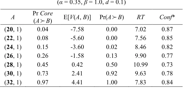
Table 1 shows how choice probabilities, confidence and response times vary in choices between a fixed
lottery and a series of sure amounts of money, when we hold the free parameters constant at α = 0.35, β =
1.0 and d = 0.1. In the context of CRRA preferences, these parameters are very much in line with estimates
derived from experimental data (e.g., Holt and Laury, 2002). The fixed lottery B (shown in the heading of
the table) offers a payoff of 40 with probability 0.8 and zero with probability 0.2, represented as (40, 0.8; 0,
0.2). The sure amounts A (shown in the first column) increase from 20 to 32 in steps of 2.
[Insert Table 1 here]
As should be expected, increasing the value of A raises the proportion of utility functions favouring
A over B, so that Pr Core(A
!
B) rises from 0.04 (when A is 20) to 0.97 (when A is 32). For the values of Afrom 20 to 26 inclusive, the mean of the core distribution of CE differences is negative, as shown in the
E[V(A, B)] column, so that Pr Lim(A
!
B) = 0.15In these cases, repeated sampling moves Pr(A
!
B) awayfrom Pr Core(A
!
B) towards 0, as entailed by Expression 6. Even when 26% of u(.) favour A, as in thefourth row where A = (26, 1), repeated sampling results in A being picked on only 13% of occasions.
However, when A increases to (28, 1), E[V(A, B)] becomes positive, so that Pr Lim(A
!
B) = 1 forthis and all higher values of A. This means that for the remaining rows in the table, repeated sampling moves
Pr(A
!
B) above Pr Core(A!
B). As a consequence, even though just 45% of u(.) favour A when A = (28, 1),A is chosen more often – in this example, in slightly more than 50% of the simulation runs, resulting in Pr(A
!
B) and Pr Core(A!
B) being on different sides of 0.5. When A = (30, 1) and is favoured by 73% of u(.),the deliberative process results in A being chosen in 92% of runs, showing again the tendency implied by
Expression 6.
The next two columns show the average response times, RT, and the average levels of Conf*. In the
rows towards the top and bottom of the table, where one or the other option is strongly favoured, RTs are
shorter and Conf* is higher. In the middle rows, where the two options are more finely balanced, more
sampling is required to reject the null hypothesis of zero difference, so that RTs become longer and Conf*
decreases. This pattern in the RTs is in line with existing empirical evidence for choices between lotteries
(see, e.g., Mosteller and Nogee, 1951; Jamieson and Petrusic, 1977; Petrusic and Jamieson, 1978; Moffatt,
2005).16 The confidence pattern is in line with the evidence found in perceptual tasks (see Pleskac and Busemeyer, 2010, for a review of this literature).
15
E[V(A, B)] has been calculated in all cases as the mean of 100,000 simulated CE differences.
16
16
3.2. Changing the Free Parameters of the Model
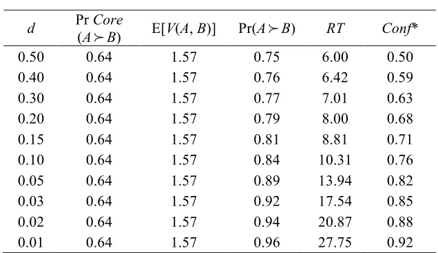
Tables 2, 3 and 4 show how the model behaves for a fixed lottery pair when each of its free parameters (α, β
and d) is progressively changed, holding all other parameters constant. For illustrative purposes, the exercise
is conducted for lottery pair {A, B}, with A = (30, 1) and B = (40, 0.8; 0, 0.2). The main results can be
summarised as follows.
Table 2 shows that when α (the mean value of r) is progressively increased so that the DM becomes
more risk averse overall, Pr(A
!
B) and Pr Core(A!
B) both increase monotonically, with Pr(A!
B) tendingto be more extreme than Pr Core(A
!
B), as implied by Expression 6. RTs tend to increase for more finelybalanced decisions, while the Conf* values show the opposite pattern.
[Insert Table 2 here]
When β is increased, widening the range of the distribution of r and producing greater variability in
V(A, B), Table 3 shows that more sampling is required to trigger a decision, entailing longer RTs and lower
Conf*.
[Insert Table 3 here]
Finally, Table 4 shows the effect of decreasing d. When d = 0.5 (so that k* = 2), Pr(A
!
B) goes fromthe Pr Core(A
!
B) level of 0.64 to 0.75 (note that since E[V(A, B)] > 0, Pr Lim(A!
B) = 1 in this case). Atthe other extreme, when d = 0.01, Pr(A
!
B) is much closer to the limiting probability of 1. Lower values ofd mean that the DM is less willing to reduce her desired level of confidence, which entails increasing the
average amount of sampling and the average RTs. So in the third row, where d = 0.3, average RTs are 7.01,
reflecting the fact that with NC = 3, the average k* is 2.34; in the sixth row, where d = 0.1, RTs are around
10. The RTs continue to rise as d falls further.
[Insert Table 4 here]
3.3. Implications for Stochastic Dominance, Transitivity, Independence and Betweenness
We now apply BREUT to some specific problems which are typical of those used in many of the
experimental studies that have motivated much of the theory development in decision making under risk and
uncertainty. We explore to what extent BREUT’s predictions do or do not correspond with various
well-known patterns. For each type of scenario, we start from theoretical results for the limiting case and then
illustrate the key patterns using simulations.
First, we show how the model behaves in conditions of first order stochastic dominance (FOSD).
Next, we consider what scope there is for violations of stochastic transitivity within the BREUT framework.
17
3.3.1. First Order Stochastic Dominance
As noted in Section 2.4, Expression 6 entails that whenever one of the lotteries is never favoured by the core
utility functions there is no amount of sampling for which that lottery will be chosen with positive
probability. This condition is trivially satisfied in the case of FOSD. Our simulations will look at the
behaviour of BREUT’s procedural measures, RT and Conf*, for different FOSD lottery pairs.
The two pairs in Table 5 involve transparent FOSD. All lotteries offer 50-50 chances of zero or a
positive payoff, with A offering a higher positive payoff than B in both pairs, 10 more in the first and 1 more
in the second, so that Pr Core(A
!
B), Pr Lim(A!
B) and Pr(A!
B) all equal 1. In spite of the larger payoffdifference in favour of A in the first pair, decisions are reached quickly and with high confidence in both
cases, resulting in virtually identical RTs and Conf*.17
[Insert Table 5 here]
3.3.2. Weak and Strong Stochastic Transitivity
In the probabilistic choice literature, a distinction has been made between weak stochastic transitivity (WST)
and strong stochastic transitivity (SST). For any three options X, Y, Z, WST requires that if Pr(X
!
Y) ≥ 0.5and Pr(Y
!
Z) ≥ 0.5, then Pr(X!
Z) ≥ 0.5. The stronger requirement in SST is that if Pr(X!
Y) ≥ 0.5 and Pr(Y!
Z) ≥ 0.5, then Pr(X!
Z) must be at least as large as the greater of those two: Pr(X!
Z) ≥ max[Pr(X!
Y),Pr(Y
!
Z)]. As Tversky and Russo (1969) showed, SST is equivalent to an independence betweenalternatives condition, whereby Pr(X
!
Z) ≥ Pr(Y!
Z) if and only if Pr(X!
W) ≥ Pr(Y!
W) for any X, Y, Zand W. That is, the relationship between the probabilities that each of two lotteries is chosen over a common
alternative should not be reversed if the alternative is changed.
Rieskamp et al. (2006) concluded that the empirical evidence of violations of WST was thin,
whereas there was plentiful evidence of violations of SST. In this subsection we show that BREUT is
consistent with WST – i.e., the only instances of violations of WST will be due to random variation rather
than to any systematic underlying tendency – but it allows systematic violations of SST of the kinds that
have been documented.
In order for there to be any tendency to violate WST in the limit, it would be necessary to generate a
case in which the mean CE differences for {X, Y} and {Y, Z} are positive but the mean CE difference for {X,
Z} is negative. However, this is clearly impossible in the limiting case, as E[V(X, Y)] + E[V(Y, Z)] = E[V(X,
Z)]. Also, any set of u(.) will yield a mean CE for each of X, Y and Z, and if CE(X) > CE(Y) and CE(Y) >
17 Empirically, even when FOSD is transparent, there are occasional violations, and there is no discernible difference in
18
CE(Z), then CE(X) > CE(Z). Thus all three differences must have the same sign, so that lower values of d
and longer RTs will tend to push Pr(X
!
Y), Pr(Y!
Z) and Pr(X!
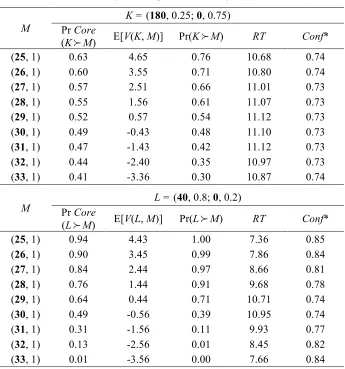
Z) progressively closer to 1.18 However, violations of SST are a different matter. This can be conveniently illustrated with anexample of the so-called Myers effect (Myers et al., 1965), which constitutes a violation of the independence
condition as specified by Tversky and Russo (1969). Table 8 shows how the probabilities of choosing
between each of two lotteries K and L and a series of sure amounts (M) change as the sure sums are
progressively increased. The independence condition applied to this case entails that any inequality between
Pr(K
!
M) and Pr(L!
M) should hold for all values of M. As Table 6 shows, this is not the case.[Insert Table 6 here]
Because K has a wider range of payoffs than L, as the sure amount M is increased, Pr Core(K
!
M) in the toppanel of Table 6 changes more slowly than Pr Core(L
!
M) in the bottom panel. For values of M below 30,Pr Core(K
!
M) < Pr Core(L!
M), while the opposite is true for M above 30. That is, violations of SST arealready present in the RP core prior to any sampling. As implied by Expression 6, the tendencies in core
probabilities are amplified by repeated sampling. Since for both lotteries the mean CE difference changes
sign as M is increased, BREUT produces even more marked violations of SST.
The patterns of RT and Conf* are again closely related to patterns in choice probabilities. In the top
panel, choice probabilities vary less over the range of M that we consider, and RT and Conf* also display
limited variation. There is more variation in choice probabilities in the bottom panel, matched by more
pronounced increases and decreases in RTs and opposite patterns in Conf*. As seen earlier, when
probabilities are more extreme (as in the bottom panel), decisions are taken more quickly and with greater
confidence than when they are closer to 0.5 (as in the bottom panel). Given the similar level of complexity
of the pairs involving K and L, when Conf* in the bottom panel is close to the level of the top panel, RT
values are also similar.
3.3.3. Implications for Independence and Betweenness
Many experimental tests of the independence axiom of deterministic EUT have used pairs of lotteries that
can be represented in Marschak-Machina (M-M) diagrams such as that shown in Figure 1 (e.g., Marschak,
1950; Machina, 1982). For any three distinct money payoffs, xh > xm > xl≥ 0, the vertical axis shows the
probability of receiving xh and the horizontal axis shows the probability of being paid xl, with any residual
probability assigned to xm. Figure 1 has been drawn for xh = 40, xm = 30 and xl = 0, with A = (30, 1), B = (40,
0.8; 0, 0.2), C = (30, 0.25; 0, 0.75), D = (40, 0.2; 0, 0.8) and E = (40, 0.2; 30, 0.75; 0, 0.05).
[Insert Figure 1 here]
18 It may be possible to produce sets of u(.) that give violations of WST under RP’s single-sample conditions, but in
19
In any such triangle, deterministic EUT entails that a DM’s preferences can be represented by a set
of linear and parallel indifference curves sloping up from south-west to north-east, with the gradient of the
lines reflecting her attitude to risk (see Machina, 1982). The straight and parallel nature of the indifference
curves entails that an EU maximiser who chooses A (respectively, B) from pair {A, B} in Figure 1, or A (E)
from pair {A, E}, would also choose C (D) from pair {C, D}. This is an implication of EUT’s independence
axiom. In addition, the fact that the indifference curves are linear implies that an EU maximiser choosing A
(respectively, B) from pair {A, B}, would also choose A (E) from pair {A, E} and E (B)from pair {E, B}.
This property is known as betweenness.
When applied to the lotteries within an M-M triangle, Becker et al.’s RP form of EUT implies that
any pair of lotteries along any straight line of a certain gradient entails the same probability of choosing the
safer option in the pair (S) over the riskier option (R), with that probability, Pr Core(S
!
R), reflecting theproportion of the DM’s vNM functions favouring S.19 The DM’s indifference curves are therefore represented by parallel straight lines with a slope such that Pr Core(S
!
R) = 0.5. So, anyone choosing Afrom pair {A, B} with some probability s, 0 ≤s ≤ 1, would also choose A from pair {A, E}, E from pair {E,
B} and C from pair {C, D} with probability s.
Experimental work dating back to Allais (1953), Kahneman and Tversky (1979) and many others
has shown that these predictions are often systematically violated. While many people tend to choose the
safer option A in pairs such as {A, B} and {A, E}, they tend to choose the riskier option D in pairs such as
{C, D}. The reversal of modal preference between pairs {A, B} and {C, D} has come to be known as the
common ratio (CR) effect, while the reversal of modal preference between {A, E} and {C, D} has come to
be known as the common consequence (CC) effect. The betweenness property has also often been found to
be violated, sometimes in the direction of the mixture being preferred over each of the two lotteries,
sometimes in the opposite direction (e.g., Becker et al, 1963b; Coombs and Huang, 1976; Bernasconi, 1994;
see Blavatskyy, 2006, for a recent overview).
We now look at BREUT’s predictions in the M-M triangle. We start by applying the limiting case of
unlimited sampling to analyse what happens when the probabilities of the best consequence are scaled down,
as in the CR scenario (Theorem 1). We then derive more general properties about the shape of the
indifference curves for cores of utility functions restricted to be either weakly concave or weakly convex
(Theorem 2), which has implications for whether or not BREUT satisfies betweenness. By combining
insights from Theorem 1 and Theorem 2, we also say more about the circumstances under which the CC
effect can be obtained (Theorem 3). We conclude the section with a series of simulations illustrating the
implications of BREUT when d > 0, which enable us to look into the behaviour of RT and Conf*.
19
20
Theorem 1
Let the core consist of N > 1 CRRA functions, i.e., functions of form 𝑈a 𝑥 = 𝑥98Wb, where ri < 1 for all iϵ {1, ..., N}, and assume that ri≠rj for at least some i, jϵ {1, ..., N}. Take any lotteries S = (xm, p; 0, 1
– p) and R = (xh, q; 0, 1 – q) for which xh> xm> 0, pϵ (0, 1], qϵ (0, 1) and for which Pr(S≻R) → 0.5 as
d→ 0. Then, for any lottery S' = (xm, σp; 0, 1 – σp) and R' = (xh, σq; 0, 1 – σq) where σϵ (0, 1), it must
be that Pr(S'≻R') → 0 as d→ 0.
Proof. See the Appendix.
Theorem 1 concerns lotteries of the form typically used in CR scenarios, S = (xm, p; 0, 1 – p) and R = (xh, q;
0, 1 – q), with xh> xm> 0. The commonly used case in which p = 1 is also allowed by Theorem 1. An
example of lotteries of this form is presented in Figure 1, in which A, B, C and D fit the descriptions of S, R,
S' and R', respectively, with p = 1, q = 0.8 and σ = 0.25.
To illustrate the intuition, suppose that Pr(S≻R) → 0.5 as d→ 0 (i.e., the decision maker is indifferent between S and R in the limit, so that E[V(S, R)] = 0) for some p≤ 1. The key result is that, for a
core made of CRRA functions, scaling the probabilities of the best outcome of each lottery down by some
factor σ always results in the DM having a strict preference for the scaled down risky lottery R'. Although
Theorem 1 starts from perfect indifference between S and R in the scaled-up pair, an immediate corollary is
that it will always be possible to obtain a strict preference in favour of S by slightly reducing q, the
probability of winning xh in R. That is, in the limit, a CR effect can always be obtained in which the DM has
a strict preference for the safer lottery in the scaled-up pair and a strict preference for riskier lottery in the
scaled-down pair. A preference reversal in the other direction does not occur for any lotteries of these forms.
Theorem 1 holds as long as there are at least two different CRRA utility functions in the core,
without any further assumption about the core distribution, such as the degree of risk aversion implied by
each function. The case of a continuous distribution (like the ones used in our simulations) can be
approximated by taking an N that is sufficiently large.
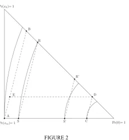
Figure 2 illustrates the implications of Theorem 1. For convenience, pairs {S, R} and {S', R'} are
drawn on (dashed) lines with the same gradient as the pairs of lotteries in Figure 1, which are also shown in
the figure. S is drawn for some p < 1 (i.e., on the bottom edge of the triangle, but away from lottery A in the
bottom-left corner). Because of the requirement that the DM is indifferent between S and R in the limit, S
and R lie on the same indifference curve (the solid line connecting S and R). In the limiting case of BREUT,
an indifference curve is the set of lotteries for which the core entails exactly the same mean CE. Theorem 1
implies that R' lies above the indifference curve passing through S'.In other words, indifference curves
become flatter as one moves towards the bottom-right corner of the triangle, in line with the often discussed
‘fanning out’ pattern. Similarly, because the S in Figure 2 has been selected arbitrarily, the theorem implies
that, to the left of S, indifference curves will be steeper. For a DM with indifference curves like those in
Figure 2, Pr Lim(A, B) = 1, Pr Lim(A, E) = 1 and Pr Lim(C, D) = 0, that is, she would display both the CR
21
[Insert Figure 2 here]
Figure 2 also serves to illustrate that, in the limiting case of BREUT, indifference curves are
typically nonlinear. The nonlinearity implies that there is no guarantee that BREUT will satisfy betweenness
in the limit. Theorem 2 sheds light on this aspect.
Theorem 2
Maintain the assumptions of Theorem 1 (i.e., the core consists of N CRRA functions, at least two of
which are distinct). Take any lotteries S = (xm, p; 0, 1 – p) and R = (xh, q; 0, 1 – q) for which xh > xm > 0,
pϵ (0, 1], qϵ (0, 1) and for which Pr(S≻R) → 0.5 as d→ 0.
Suppose that all utility functions are (weakly) concave, i.e., 0 ≤ri < 1 for all iϵ {1, ..., N}. Then Pr(S≻
ωS + (1 – ω)R) → 1 and Pr(R≻ωS + (1 – ω)R) → 1 as d→ 0, with ωϵ (0, 1).20
Suppose that all utility functions are (weakly) convex, i.e., ri≤ 0 for all iϵ {1, ..., N}. Then Pr(S≻ωS +
(1 – ω)R) → 0 and Pr(R≻ωS + (1 – ω)R) → 0 as d→ 0.
Proof. See the Appendix.
According to Theorem 2, if there are only (weakly) concave utility functions in the core, BREUT’s
indifference curves are always concave. This is the case depicted in Figure 2. Note that, since there must be
at least two distinct utility functions in the core (as assumed in Theorem 1), the weak concavity requirement
entails that there will be at least one strictly concave function. The key result is that any mixture of two
lotteries, S = (xm, p; 0, 1 – p) and R = (xh, q; 0, 1 – q), that lie on the same indifference curve will be less
preferred than either S or R. However, since the DM is assumed to be exactly indifferent between the two
mixed lotteries, the degree of concavity of the indifference curves will typically be very small (unless the
core is made of very extreme functions). This limits the room for observing violations of betweenness when
sampling is limited (see our simulations below).21 If the core contains only (weakly) convex utility functions, then indifference curves will be convex and any mixture of S and R will be preferred to both. If
there are both concave and convex utility functions in the core, the exact shape of the indifference curves
will depend on the balance between concave and convex functions and on how extreme these are.22
20 Here and in the Appendix, we will use the notation ωS + (1 – ω)R to indicate a lottery mixture of ω times the
probability of the prizes inside the support of lottery S and 1– ω times the probability of the prizes in lottery R.
21
Note that Figure 2 is a sketch with an accentuated degree of concavity to illustrate the implications of our theorems more clearly.
22
22
An implication of Theorems 1 and 2 is that, while the CR effect will always be observed in the limit,
for any core, the same is not guaranteed for the CC effect. But the effect will always be found in the limit if
the core does not contain convex utility functions (the case illustrated in Figure 2), as detailed in Theorem 3.
Theorem 3
Maintain the assumptions of Theorem 1 (i.e., the core consists of N CRRA functions, at least two of
which are distinct). Suppose that all utility functions are (weakly) concave, i.e., 0 ≤ri < 1 for all iϵ {1,
..., N}. Take any lotteries T = (xm, 1) and Z = (xh, q1; xm, q2; 0, 1 – q1 – q2) for which xh > xm > 0, q1, q2ϵ
(0, 1), q1 + q2 < 1 and Pr(T≻Z) → 0.5 as d→ 0. Then it must be that for T' = (xm, 1 – q2; 0, q2) and Z' =
(xh, q1; 0, 1 – q1), Pr(T'≻Z') → 0 as d→ 0.
Proof. See the Appendix.
All these results hold for the limiting case of unlimited sampling, and we also know from Expression
6 that, for any {S, R} pair, any pattern in Pr Lim(S, R) will eventually emerge in Pr(S, R) with sufficient
sampling. The simulations reported in Table 7 explore the implications of the general form of BREUT for
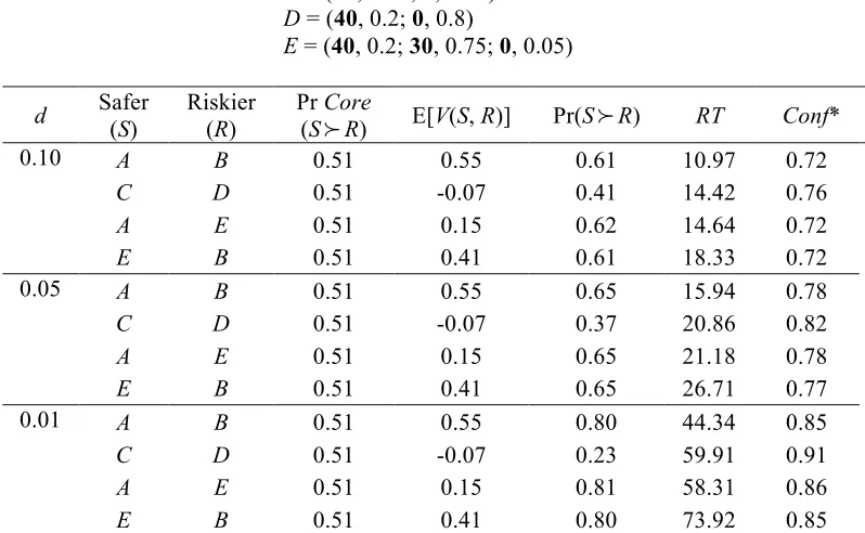
the four lottery pairs shown in Figure 1, using three values of d (0.1, 0.05 and 0.01), and setting a = 0.23, β
= 1.0. These levels of risk aversion, which are not atypical in experiments, have been chosen to obtain
values of Pr Core(S
!
R) close to 0.5, in line with the assumptions of our theorems. This has the advantageof allowing us to illustrate the main implications of our model more clearly. Using positive values of d will
also entail predictions for RT and Conf*.
[Insert Table 7 here]
We start by looking at the E[V(S, R)] column of Table 7, which links up to the limiting case. For all
pairs except {C, D}, E[V(S, R)] is positive, so we can expect that in each of these pairs the safer option will
be chosen with probability 1 in the limit. The negative value for {C, D} implies that in the limit the riskier
option will be chosen with probability 1, in line with both the CR and CC effects. Because of the signs of
E[V(S, R)] and the fact that Pr Core(S
!
R) = 0.51, Expression 6 implies that, with limited sampling, therewill be a reversal of modal choice in both the CR and CC scenarios, as we see in all panels of Table 7. In
addition, Pr(S
!
R) moves further away from 0.5 as d decreases and the DM samples more. As can beexpected, as d gets smaller, RTs increase on average; correspondingly, the DM makes her choices with
higher confidence.
In all the cases presented in Table 7, there are no violations of probabilistic betweenness (in all three
panels, the choice probabilities for pairs {A, B}, {A, E} and {E, B} are virtually identical). From the E[V(S,
R)] column, we know that Pr Lim(A, B) = 1, Pr Lim(A, E) = 1 and Pr Lim(E, B) = 1. We know from Theorem
2 that in order for violations of betweenness to be guaranteed in the limit, the core of