Distributed Representations of Geographically Situated Language
David Bamman Chris Dyer Noah A. Smith School of Computer Science
Carnegie Mellon University Pittsburgh, PA 15213, USA
{dbamman,cdyer,nasmith}@cs.cmu.edu
Abstract
We introduce a model for incorporating contextual information (such as geogra-phy) in learning vector-space representa-tions ofsituated language. In contrast to approaches to multimodal representation learning that have used properties of the objectbeing described (such as its color), our model includes information about the subject (i.e., the speaker), allowing us to learn the contours of a word’s meaning that are shaped by the context in which it is uttered. In a quantitative evaluation on the task of judging geographically in-formed semantic similarity between repre-sentations learned from 1.1 billion words of geo-located tweets, our joint model out-performs comparable independent models that learn meaning in isolation.
1 Introduction
The vast textual resources used in NLP – newswire, web text, parliamentary proceedings – can encourage a view of language as a disembod-ied phenomenon. The rise of social media, how-ever, with its large volume of text paired with in-formation about its author and social context, re-minds us that each word is uttered by a particular person at a particular place and time. In short: lan-guage issituated.
The coupling of text with demographic infor-mation has enabled computational modeling of linguistic variation, including uncovering words and topics that are characteristic of geographical regions (Eisenstein et al., 2010; O’Connor et al., 2010; Hong et al., 2012; Doyle, 2014), learning correlations between words and socioeconomic variables (Rao et al., 2010; Eisenstein et al., 2011; Pennacchiotti and Popescu, 2011; Bamman et al., 2014); and charting how new terms spread geo-graphically (Eisenstein et al., 2012). These models
can tell us thathellawas (at one time) used most often by a particular demographic group in north-ern California, echoing earlier linguistic studies (Bucholtz, 2006), and that wicked is used most often in New England (Ravindranath, 2011); and they have practical applications, facilitating tasks like text-based geolocation (Wing and Baldridge, 2011; Roller et al., 2012; Ikawa et al., 2012). One desideratum that remains, however, is how the meaningof these terms is shaped by geographical influences – whilewicked is used throughout the United States to meanbadorevil(“he is a wicked man”), in New England it is used as an adverbial intensifier (“my boy’s wicked smart”). In lever-aging grounded social media to uncover linguistic variation, what we want to learn is how a word’s meaning is shaped by its geography.
In this paper, we introduce a method that ex-tends vector-space lexical semantic models to learn representations of geographically situated language. Vector-space models of lexical seman-tics have been a popular and effective approach to learning representations of word meaning (Lin, 1998; Turney and Pantel, 2010; Reisinger and Mooney, 2010; Socher et al., 2013; Mikolov et al., 2013,inter alia). In bringing in extra-linguistic in-formation to learn word representations, our work falls into the general domain of multimodal learn-ing; while other work has used visual informa-tion to improve distributed representainforma-tions (An-drews et al., 2009; Feng and Lapata, 2010; Bruni et al., 2011; Bruni et al., 2012a; Bruni et al., 2012b; Roller and im Walde, 2013), this work generally exploits information about the object be-ing described (e.g., strawberryand a picture of a strawberry); in contrast, we use information about thespeaker to learn representations that vary ac-cording to contextual variables from the speaker’s perspective. Unlike classic multimodal systems that incorporate multiple active modalities (such as gesture) from a user (Oviatt, 2003; Yu and
...
W
X
Main Alabama Alaska Arizona Arkansas
h
[image:2.595.93.509.61.212.2]o
Figure 1: Model. Illustrated are the input dimensions that fire for a single sample, reflecting a particular word (vocabulary item #2) spoken in Alaska, along with a single output. Parameter matrixWconsists of the learned low-dimensional embeddings.
Ballard, 2004), our primary input is textual data, supplemented with metadata about the author and the moment of authorship. This information en-ables learning models of word meaning that are sensitive to such factors, allowing us to distin-guish, for example, between the usage ofwicked in Massachusetts from the usage of that word else-where, and letting us better associate geographi-cally grounded named entities (e.g, Boston) with their hypernyms (city) in their respective regions.
2 Model
The model we introduce is grounded in the distri-butional hypothesis (Harris, 1954), that two words are similar by appearing in the same kinds of con-texts (where “context” itself can be variously de-fined as the bag or sequence of tokens around a tar-get word, either by linear distance or dependency path). We can invoke the distributional hypothe-sis for many instances of regional variation by ob-serving that such variants often appear in similar contexts. For example:
• my boy’swickedsmart • my boy’shellasmart • my boy’sverysmart
Here, all three variants can often be seen in an im-mediately pre-adjectival position (as is common with intensifying adverbs).
Given the empirical success of vector-space rep-resentations in capturing semantic properties and their success at a variety of NLP tasks (Turian et al., 2010; Socher et al., 2011; Collobert et al., 2011; Socher et al., 2013), we use a simple, but state-of-the-art neural architecture (Mikolov et al., 2013) to learn low-dimensional real-valued
repre-sentations of words. The graphical form of this model is illustrated in figure 1.
This model corresponds to an extension of the “skip-gram” language model (Mikolov et al., 2013) (hereafter SGLM). Given an input sentence
sand a context window of sizet, each wordsiis conditioned on in turn to predict the identities of all of the tokens within twords around it. For a vocabulary V, each input word si is represented as a one-hot vectorwi of length|V|. The SGLM has two sets of parameters. The first is the rep-resentation matrixW ∈ R|V|×k, which encodes the real-valued embeddings for each word in the vocabulary. A matrix multiplyh = w>W,∈ Rk serves to index the particular embedding for word
w, which constitutes the model’s hidden layer. To predict the value of the context word y (again, a one-hot vector of dimensionality|V|), this hidden representationhis then multiplied by a second pa-rameter matrixX ∈R|V|×k. The final prediction over the output vocabulary is then found by pass-ing this resultpass-ing vector through the softmax func-tiono=softmax(Xh), giving a vector in the|V |-dimensional unit simplex. Backpropagation using (input x, output y) word tuples learns the values ofW (the embeddings) andX(the output param-eter matrix) that maximize the likelihood ofy(i.e., the context words) conditioned onx(i.e., thesi’s). During backpropagation, the errors propagated are the difference between o (a probability distribu-tion withkoutcomes) and the true (one-hot) out-puty.
Let us define a set of contextual variables C; in the experiments that follow, C is com-prised solely of geographical state Cstate =
month, day of week, or other demographic vari-ables of the speaker. Let|C|denote the sum of the cardinalities of all variables in C (i.e., 51 states, including the District of Columbia). Rather than using a single embedding matrixW that contains low-dimensional representations for every word in the vocabulary, we define a global embedding ma-trixWmain ∈ R|V|×k and an additional|C|such
matrices (each again of size|V| ×k, which cap-ture the effect that each variable value has on each word in the vocabulary. Given an input wordw
and set of active variable values A (e.g., A = {state = MA}), we calculate the hidden layer
h as the sum of these independent embeddings:
h=w>Wmain+P
a∈Aw>Wa. While the word
wickedhas a common low-dimensional represen-tation in Wmain,wicked that is invoked for every
instance of its use (regardless of the place), the corresponding vector WMA,wicked indicates how
that common representation should shift in k -dimensional space when used in Massachusetts. Backpropagation functions as in standard SGLM, with gradient updates for each training example {x, y}touching not onlyWmain(as in SGLM), but
all activeWAas well.
The additional W embeddings we add lead to an increase in the number of total parameters by a factor of |C|. To control for the extra degrees of freedom this entails, we add squared`2 regu-larization to all parameters, using stochastic gra-dient descent for backpropagation with minibatch updates for the regularization term. As in Mikolov et al. (2013), we speed up computation using the hierarchical softmax (Morin and Bengio, 2005) on the output matrixX.
This model defines a joint parameterization over all variable values in the data, where information from data originating in California, for instance, can influence the representations learned for Wis-consin; a naive alternative would be to simply train individual models on each variable value (a “Cal-ifornia” model using data only from California, etc.). A joint model has threea prioriadvantages over independent models: (i) sharing data across variable values encourages representations across those values to be similar; e.g., whilecitymay be closer toBostonin Massachusetts andChicagoin Illinois, in both places it still generally connotes amunicipality; (ii) such sharing can mitigate data sparseness for less-witnessed areas; and (iii) with a joint model, all representations are guaranteed to
be in the same vector space and can therefore be compared to each other; with individual models (each with different initializations), word vectors across different states may not be directly com-pared.
3 Evaluation
We evaluate our model by confirming its face validity in a qualitative analysis and estimating its accuracy at the quantitative task of judging geographically-informed semantic similarity. We use 1.1 billion tokens from 93 million geolocated tweets gathered between September 1, 2011 and August 30, 2013 (approximately 127,000 tweets per day evenly sampled over those two years). This data only includes tweets that have been ge-olocated to state-level granularity in the United States using high-precision pattern matching on the user-specified location field (e.g., “new york ny” → NY, “chicago” → IL, etc.). As a pre-processing step, we identify a set of target mul-tiword expressions in this corpus as the maximal sequence of adjectives + nouns with the highest pointwise mutual information; in all experiments described below, we define the vocabulary V as the most frequent 100,000 terms (either unigrams or multiword expressions) in the total data, and set the dimensionality of the embeddingk = 100. In all experiments, the contextual variable is the ob-served US state (including DC), so that|C|= 51; the vector space representation of wordwin state
sisw>Wmain+w>Ws.
3.1 Qualitative Evaluation
To illustrate how the model described above can learn geographically-informed semantic represen-tations of words, table 1 displays the terms with the highest cosine similarity towicked in Kansas and Massachusetts after running our joint model on the full 1.1 billion words of Twitter data; while wickedin Kansas is close to other evaluative terms likeevilandpureand religious terms likegodsand spirit, in Massachusetts it is most similar to other intensifiers likesuper,ridiculouslyandinsanely.
Kansas Massachusetts
term cosine term cosine
wicked 1.000 wicked 1.000
evil 0.884 super 0.855
pure 0.841 ridiculously 0.851 gods 0.841 insanely 0.820 mystery 0.830 extremely 0.793 spirit 0.830 goddamn 0.781 king 0.828 surprisingly 0.774
above 0.825 kinda 0.772
[image:4.595.95.271.60.190.2]righteous 0.823 #sarcasm 0.772 magic 0.822 sooooooo 0.770 Table 1: Terms with the highest cosine similarity towicked in Kansas and Massachusetts.
California New York
term cosine term cosine
city 1.000 city 1.000
valley 0.880 suburbs 0.866
bay 0.874 town 0.855
downtown 0.873 hamptons 0.852 chinatown 0.854 big city 0.842 south bay 0.854 borough 0.837 area 0.851 neighborhood 0.835 east bay 0.845 downtown 0.827 neighborhood 0.843 upstate 0.826 peninsula 0.840 big apple 0.825 Table 2: Terms with the highest cosine similarity tocityin California and New York.
(New York City’s term of administrative division).
3.2 Quantitative Evaluation
As a quantitative measure of our model’s perfor-mance, we consider the task of judging semantic similarity among words whose meanings are likely to evoke strong geographical correlations. In the absence of a sizable number of linguistically in-teresting terms (likewicked) that are known to be geographically variable, we consider the proxy of estimating the named entities evoked by specific terms in different geographical regions. As noted above, geographic terms likecityprovide one such example: in Massachusetts we expect the termcity to be more strongly connected to grounded named entities like Boston than to other US cities. We consider seven categories for which we can rea-sonably expect the connotations of each term to vary by geography; in each case, we calculate the distance between two termsx andy using repre-sentations learned for a given state (δstate(x, y)).
1. city. For each state, we measure the distance between the word city and the state’s most populous city; e.g.,δAZ(city,phoenix). 2. state. For each state, the distance between
the word state and the state’s name; e.g.,
δWI(state,wisconsin).
3. football. For all NFL teams, the distance be-tween the wordfootballand the team name; e.g.,δIL(football,bears).
4. basketball. For all NBA teams from a US state, the distance between the word basketball and the team name; e.g.,
δFL(basketball,heat).
5. baseball. For all MLB teams from a US state, the distance between the wordbaseball and the team name; e.g.,δIL(baseball,cubs),
δIL(baseball,white sox).
6. hockey. For all NHL teams from a US state, the distance between the wordhockeyand the team name; e.g.,δPA(hockey,penguins). 7. park. For all US national parks, the distance
between the word park and the park name; e.g.,δAK(park,denali).
Each of these questions asks the following: what words are evoked for a given target word (like football)? While football may everywhere evoke similar sports like baseball or soccer or more specific football-related terms like touch-downorfield goal, we expect that particular sports teams will be evoked more strongly by the word footballin their particular geographical region: in Wisconsin, football should evoke packers, while in Pennsylvania, football evokes steelers. Note that this is not the same as simply asking which sports team is most frequently (or most character-istically) mentioned in a given area; by measuring the distance to a target word (football), we are at-tempting to estimate the varying strengths of asso-ciation between concepts in different regions.
For each category, we measure similarity as the average cosine similarity between the vector for the target word for that category (e.g.,city) and the corresponding vector for each state-specific an-swer (e.g., chicago for IL; boston for MA). We compare three different models:
1. JOINT. The full model described in section 2, in which we learn a global representation for each word along with deviations from that common representation for each state. 2. INDIVIDUAL. For comparison, we also
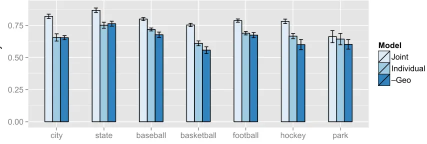
[image:4.595.81.282.232.363.2]0.00 0.25 0.50 0.75
city state baseball basketball football hockey park
si
mi
la
rit
y Model
Joint
Individual
[image:5.595.81.508.72.216.2]–Geo
Figure 2: Average cosine similarity for all models across all categories, with 95% confidence intervals on the mean.
data with 11,604,637 tweets; Wyoming has the least with 47,503 tweets.
3. –GEO. We also train a single model on all of the training data, but ignore any state meta-data. In this case the distanceδbetween two terms is their overall distance within the en-tire United States.
As one concrete example of these differences between individual data points, the cosine similar-ity between city and seattle in the –GEO model is0.728(seattleis ranked as the 188th most sim-ilar term to city overall); in the INDIVIDUAL model using only tweets from Washington state,
δW A(city, seattle) = 0.780 (rank #32); and in the JOINTmodel, using information from the en-tire United States with deviations for Washington,
δW A(city, seattle) = 0.858(rank #6). The over-all similarity for the city category of each model is the average of 51 such tests (one for each city).
Figure 2 present the results of the full evalua-tion, including 95% confidence intervals for each mean. While the two models that include ge-ographical information naturally outperform the model that does not, the JOINT model generally far outperforms the INDIVIDUAL models trained on state-specific subsets of the data.1A model that
can exploit all of the information in the data, learn-ing core vector-space representations for all words along with deviations for each contextual variable, is able to learn more geographically-informed rep-resentations for this task than strict geographical models alone.
1This result is robust to the choice of distance metric; an evaluation measuring the Euclidean distance between vectors shows the JOINTmodel to outperform the INDIVIDUALand –GEOmodels across all seven categories.
4 Conclusion
We introduced a model for leveraging situational information in learning vector-space representa-tions of words that are sensitive to the speaker’s social context. While our results use geographical information in learning low-dimensional represen-tations, other contextual variables are straightfor-ward to include as well; incorporating effects for time – such as time of day, month of year and ab-solute year – may be a powerful tool for reveal-ing periodic and historical influences on lexical se-mantics.
Our approach explores the degree to which ge-ography, and other contextual factors, influence word meaning in addition to frequency of usage. By allowing all words in different regions (or more generally, with different metadata factors) to ex-ist in the same vector space, we are able com-pare different points in that space – for example, to ask what terms used in Chicago are most simi-lar tohot dogin New York, or what word groups shift together in the same region in comparison to the background (indicating the shift of an en-tire semantic field). All datasets and software to support these geographically-informed represen-tations can be found at: http://www.ark. cs.cmu.edu/geoSGLM.
5 Acknowledgments
References
Mark Andrews, Gabriella Vigliocco, and David Vin-son. 2009. Integrating experiential and distribu-tional data to learn semantic representations. Psy-chological Review, 116(3):463–498.
David Bamman, Jacob Eisenstein, and Tyler Schnoe-belen. 2014. Gender identity and lexical variation in social media. Journal of Sociolinguistics, 18(2). Elia Bruni, Giang Binh Tran, and Marco Baroni. 2011.
Distributional semantics from text and images. In
Proc. of the Workshop on Geometrical Models of Natural Language Semantics.
Elia Bruni, Gemma Boleda, Marco Baroni, and Nam-Khanh Tran. 2012a. Distributional semantics in technicolor. InProc. of ACL.
Elia Bruni, Jasper Uijlings, Marco Baroni, and Nicu Sebe. 2012b. Distributional semantics with eyes: Using image analysis to improve computational
rep-resentations of word meaning. InProc. of the ACM
International Conference on Multimedia.
Mary Bucholtz. 2006. Word up: Social meanings of slang in California youth culture. In Jane Goodman
and Leila Monaghan, editors,A Cultural Approach
to Interpersonal Communication: Essential
Read-ings, Malden, MA. Blackwell.
Ronan Collobert, Jason Weston, L´eon Bottou, Michael Karlen, Koray Kavukcuoglu, and Pavel Kuksa. 2011. Natural language processing (almost) from
scratch. Journal of Machine Learning Research,
12:2493–2537.
Gabriel Doyle. 2014. Mapping dialectal variation by querying social media. InProc. of EACL.
Jacob Eisenstein, Brendan O’Connor, Noah A. Smith, and Eric P. Xing. 2010. A latent variable model for geographic lexical variation. InProc. of EMNLP. Jacob Eisenstein, Noah A. Smith, and Eric P. Xing.
2011. Discovering sociolinguistic associations with structured sparsity. InProc. of ACL.
Jacob Eisenstein, Brendan O’Connor, Noah A. Smith, and Eric P. Xing. 2012. Mapping the geographical diffusion of new words. arXiv, abs/1210.5268. Yansong Feng and Mirella Lapata. 2010. Visual
in-formation in semantic representation. In Proc. of
NAACL.
Zellig Harris. 1954. Distributional structure. Word,
10(23):146–162.
Liangjie Hong, Amr Ahmed, Siva Gurumurthy, Alexander J. Smola, and Kostas Tsioutsiouliklis. 2012. Discovering geographical topics in the Twit-ter stream. InProc. of WWW.
Yohei Ikawa, Miki Enoki, and Michiaki Tatsubori. 2012. Location inference using microblog
mes-sages. InProc. of WWW.
Dekang Lin. 1998. Automatic retrieval and clustering
of similar words. InProc. of COLING-ACL.
Tomas Mikolov, Kai Chen, Greg Corrado, and Jeffrey Dean. 2013. Efficient estimation of word represen-tations in vector space. InProc. of ICLR.
Frederic Morin and Yoshua Bengio. 2005. Hierarchi-cal probabilistic neural network language model. In Robert G. Cowell and Zoubin Ghahramani, editors,
Proc. of AISTATS.
Brendan O’Connor, Jacob Eisenstein, Eric P. Xing, and Noah A. Smith. 2010. Discovering demographic
language variation. InNIPS Workshop on Machine
Learning and Social Computing.
Sharon Oviatt. 2003. Multimodal interfaces.
In Julie A. Jacko and Andrew Sears, editors,
The Human-computer Interaction Handbook, pages 286–304, Hillsdale, NJ, USA. L. Erlbaum Asso-ciates Inc.
Marco Pennacchiotti and Ana-Maria Popescu. 2011. Democrats, Republicans and Starbucks afficionados: User classification in Twitter. InProc. of KDD. Delip Rao, David Yarowsky, Abhishek Shreevats, and
Manaswi Gupta. 2010. Classifying latent user
at-tributes in Twitter. In Proc. of the Workshop on
Search and Mining User-generated Contents. Maya Ravindranath. 2011. A wicked good reason to
study intensifiers in New Hampshire. InNWAV 40.
Joseph Reisinger and Raymond J. Mooney. 2010. Multi-prototype vector-space models of word mean-ing. InProc. of NAACL.
Stephen Roller and Sabine Schulte im Walde. 2013. A multimodal LDA model integrating textual, cogni-tive and visual modalities. InProc. of EMNLP. Stephen Roller, Michael Speriosu, Sarat Rallapalli,
Benjamin Wing, and Jason Baldridge. 2012. Super-vised text-based geolocation using language models
on an adaptive grid. InProc. of EMNLP-CoNLL.
Richard Socher, Jeffrey Pennington, Eric H. Huang, Andrew Y. Ng, and Christopher D. Manning. 2011. Semi-supervised recursive autoencoders for predict-ing sentiment distributions. InProc. of EMNLP.
Richard Socher, John Bauer, Christopher D. Manning, and Ng Andrew Y. 2013. Parsing with composi-tional vector grammars. InProc. of ACL.
Joseph Turian, Lev Ratinov, and Yoshua Bengio. 2010. Word representations: A simple and general method for semi-supervised learning. InProc. of ACL.
Benjamin P. Wing and Jason Baldridge. 2011. Sim-ple supervised document geolocation with geodesic grids. InProc. of ACL.
Chen Yu and Dana H. Ballard. 2004. A multimodal learning interface for grounding spoken language in
sensory perceptions. ACM Transactions on Applied