Structural Change and Poverty Reduction at Sub State Levels in India

Munich Personal RePEc Archive

Structural Change and Poverty

Reduction at Sub-State Levels in India

Sen Gupta, Abhijit and More, Vishal and Gupta, Kanupriya

Interlink Advisors

July 2016

Online at

https://mpra.ub.uni-muenchen.de/72740/

Structural Change and Poverty Reduction at Sub-State Levels in India

*

Abhijit Sen Gupta

†

Vishal More

‡

Kanupriya Gupta

§

Abstract

Over the last two decades India has witnessed a significant rise in growth rate compared to historical levels. In this study, we investigate the pattern and nature of growth, and its implication for poverty reduction in India. In particular, we focus on the extent to which, structural change defined as changes in the composition of the economy in terms of key sectors, their employment and productivity, has an impact on poverty reduction. The paper is first of its kind in focusing on these issue at the sub-state level, which is important given the large size of Indian states that mask a great deal of heterogeneity. Moreover, the paper focuses on alternate definitions of structural change, including for the first differentiating between productivity increases in India arising from workers moving into above average productivity level sectors from workers moving to sectors that are experiencing positive productivity growth. The paper finds that while improving sectoral productivity is important for poverty reduction, there is a strong link between shift of workers into sectors witnessing an increase in poverty and poverty reduction. Thus poverty reduction requires generating jobs in dynamic sectors that are witnessing productivity growth as well as imparting adequate skills to the workforce to make them employable in these sectors.

Keywords: Structural change, poverty reduction, reallocation effect and labour productivity

JEL Classification: I32; J24; J62; R11.

*

The views expressed in this publication are those of the authors and do not necessarily reflect the views and policies of the Asian Development Bank (ADB) or its Board of Governors or the governments they represent.

†

Economist, India Resident Mission, Asian Development Bank, New Delhi, India. Email: [email protected].

‡ _{Founder and Managing Partner, Interlink Advisors, New Delhi, India. Email: [email protected].} § _{Project Officer (Results Management), India Resident Mission, Asian Development Bank, New Delhi,}

2

1.

Introduction

India’s economy started experiencing robust growth in the 1980s, following 3 decades of slow growth. Average annual GDP growth increased from 5.6% in the 1980s to 5.9% in the 1990s, and further to 7.3% in the 2000s. As a result, India’s per capita GDP increased more than five folds during these three decades to almost USD1500 by 2015, enabling its transition into a middle income country. Moreover, the growth has been broadly inclusive. Poverty rates based on World Bank’s USD1.90 a day poverty line, exhibit a decline from 52.6% in 1983 to 21.3% in 2011-12. A reduction of slightly higher magnitude is witnessed using the national poverty lines, according to which poverty rates have more than halved from 45.3% in 1993-94 to 21.9% in 2011-12.

While these trends are encouraging, they mask a great deal of divergence at the sub-national level. At the state level, per capita GDP of Haryana, one of the richest states in India, is nearly 3.7 times that of the poorest state of Bihar. International comparison implies that while Haryana’s per capita GDP is close to that of Vietnam, Bihar’s is closer to that of Eritrea or Guniea-Bissau. A further disaggregated analysis at the district level indicates an even greater degree of divergence. The district of Gurgaon in Haryana has a per capita GDP, which in 2011, was 28 times that of the poorest district of Madhepura in Bihar. Again, in international terms, this would imply a comparison between People’s Republic of China and Burundi, with the latter being the lowest ranked economy in terms of per capita income in 2011.

Similarly, despite a secular decline in poverty rates, some states continue to have a significant proportion of their population below the poverty line. For example, close to 40% of the population in Chhattisgarh continue to live in abject poverty, while in Bihar the ratio is close to 33.7%1. At the other extreme, Himachal Pradesh, Kerala and Punjab have less than 8% of the population living below the poverty line. What this means is that, even as India witnessed rapid growth and poverty reduction since 1990s, it has not been able to eliminate the large disparities across states and regions, which continue to pose a challenge for policy makers.

In this paper, we investigate the pattern and nature of growth, and its implication for poverty reduction in India. In particular, we focus on the extent to which, structural change defined as changes in the composition of the economy in terms of key sectors, their employment and productivity, has an impact on poverty reduction. The underlying theme is that shift of resources from low productivity sector into high productivity sector not only facilitates growth but also reduces poverty, as average wages tend to be higher in sectors with higher productivity.

While several papers have looked into the extent of structural change in India, with a few looking at the relationship between structural change and poverty reduction, this paper’s contribution is threefold. Firstly, while much of the existing literature evaluates the extent of structural change at the aggregate country level or at the state level, this paper undertakes an analysis at the sub-state level. The latter becomes important given the large size of Indian states, which can mask a great deal of heterogeneity. Secondly, we extend the existing analysis to 2011-12, covering the period 2009-10 to 2011-12, when India witnessed the fastest pace of poverty reduction. Finally, the paper analyses various alternate definitions of structural

1

3

change. These range from indices that define structural change as the aggregate shifts in sectoral shares, to structural change being associated with productivity increase, where changes in employment shares of the sector are weighted by productivity levels. For the first time, this paper differentiates between productivity increases in India arising from workers moving into above average productivity level sectors from workers moving to sectors that are experiencing positive productivity growth.

We focus our attention on 18 major states of India, which together account for nearly 84% of output, 96.7% of employment and 93.7% of people living below the poverty

line. We analyze the 55th, 61st and 68th rounds undertaken in 1999-00, 2004-05 and

2011-12. The choice of the initial period is driven by the availability of data on district domestic product, while the choice of the final period is based on the most recent data on poverty estimates This period coincides with the high growth period in India, with India’s GDP growing at an average annual rate of 7.4%, and poverty declining from 45.3% in 1993-94 to 21.9% in 2011-12.

2.

A Brief Review of the Existing Literature

The process of structural transformation typically referring to the reallocation of labour across sectors over time has been extensively well documented with notable early contributions from Clark (1957), Chenery (1960), Kuznets (1966) and many recent contributions including Duarte and Restuccia (2010), McMillian et al (2014). The early work starts with analysis of structural transformation of the global economy as a whole. The appearance of the new data sets and long time series at the country level over time made it worthwhile to study the role of structural change at the regional level and the country level. Later contribution is important as the nature and speed with which structural transformation takes place differs across regions/countries and can be an important contributor to overall country’s economic growth and poverty reduction. In fact, this paper is an attempt to study the role of structural transformation in India at sub-state level.

At the global level, McGregor and Verspagen (2016) analyzed the role of structural transformation and found that at levels of GDP per capita below $5000, agriculture is the dominating sector and its share in the employment declines as GDP per capita increases. Another structural break takes place at around $12000 when the share in the manufacturing sector declines. However, this process of structural transformation and growth differs across regions and countries which in turn are influenced by various factors (Felipe et.al (2015); Sen (2016)).

4

competitive or undervalued exchange rates and labour market flexibility contributes to growth enhancing structural change. Ungor (2015) compared Latin America with East Asia and reported similar findings. Latin American countries exhibit much slower de-agriculturalization than East Asian countries, while the manufacturing employment share has been almost stagnant in Latin America but exhibits a hump shaped pattern among East Asian countries.

In the Asian context, the pace of structural transformation has differed widely across countries. The so-called Asian Tigers (the Republic of Korea; Taipei, China; Singapore; Hong Kong, China) were the first generation of postwar developing countries that managed to make the transition to developed economies by going through a deep process of structural transformation. (Felipe, et al. (2014)). However, there are other Asian countries, which have not done as well in terms of structural transformation even when they enjoyed growth success.

Betts et al. (2013) and Teignier (2013) studied the path of structural transformation in South Korea during its growth miracle period. The studies found a vital role of comparative advantage and international trade in accelerating the transition out of agriculture into industry and services. Dekle and Vandenbroucke (2012) studied structural transformation in China during 1978–2003 and found that differential sectoral productivity growth and the reduction of the relative size of the Chinese government caused most of the structural transformation, but mobility frictions (like the household registration system known as hukou system) slowed the movement out of agriculture.

Various studies have shown that structural transformation in India has been very slow and is atypical in the Asian context (Kocchar et al (2006), Sen (2014)). This is because of the various reasons—fall in share of labour-intensive manufacturing in total output over time (Sen (2009)), shift in economic activity towards services and not manufacturing as in the case of other Asian high-growth economies and dualism of India manufacturing sector with rising gap of the labour productivity in the formal sector vis-à-vis informal sector. In studying the role of structural transformation in India during 1980-2005, Verma (2012) also found that Total Factor Productivity growth was fastest in services. This growth pattern differs not only from the historical growth experience of developed countries such as United Kingdom, France and the United States but also from many Asian economies.

The literature on structural transformation identified two broad factors affecting role of structural transformation in various economies—government failures and market failures (Sen 2016). The first relates to government failure including labour regulations/policies (Besley and Burgess (2004), Botero et al (2004) and Fallon and Lucas (1993)), land policies (Studwell (2013)) and product market regulations (World Bank (2013)) which can impede the functioning of factor and product markets affecting the reallocation of labour from low-productivity sectors to high productivity sectors. Market failures such as coordination problems in investments (Lin and Monga (2010)), credit market imperfections (Stiglitz and Weiss (1981); Sen and Vaidya (1997)) and human capital formation are other potential reasons which affect the demand for labour in high-productivity sectors and the supply of labour from low-productivity sectors.

3.

Extent of Structural Change across Regions

5

analysis should be conducted at the district level, there are some difficulties. Out of the nearly 15,000 observations available (451 districts, 11 sectors and 3 years), nearly 3000 or about 30% of the observations have a positive sectoral district domestic product without having a corresponding employment figure. This could be driven by a small sample size of sectors that traditionally employ a limited set of workers. This makes calculating labour productivity difficult. To overcome this, we conduct our analysis at the region level, which is aggregation of districts. The 18 states that we focus on are accordingly decomposed into 53 regions. In the case of smaller states of Jharkhand, Chhattisgarh and Uttarakhand, the entire states can be considered as a region, the larger states are divided into two or more regions. In particular, the region comprises groups of districts that form contiguous clusters and

in most instances have socio-cultural relevance.2

[image:6.612.101.507.337.498.2]

Even at the region level, there are 11 instances of regions having sectors with positive output but missing employment. Closer inspection reveals that in 10 such instances, the sectors were ‘mining and quarrying’ or ‘electricity, gas and water supply’. Given the low employment potential of these sectors, we drop these sectors3. Another instance is the registered manufacturing sector in Assam Hills region. We drop this region from our analysis, and hence focus on 9 sectors across 52 regions.

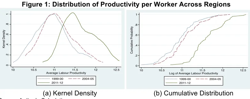
Figure 1: Distribution of Productivity per Worker Across Regions

(a) Kernel Density (b) Cumulative Distribution

Source: Author’s Calculations

Figure 1 plots the kernel density and the cumulative distribution of log of average productivity per worker across 52 regions over the periods 1999-00, 2004-05 and 2011-12. Several characteristics are evident. First, as expected there is a rightward shift of the distribution across the years, implying that productivity per worker increased between these periods at each point in the distribution. While average productivity grew at an average annual rate of 2.8% during the period 1999-00 to 2004-05, it accelerated sharply to 7.9% during 2004-05 to 2011-12. This has been associated with reducing variance, implying some degree of convergence across the regions over the years. Second, there is a slight increase in kurtosis, in 2011-12, compared to 2004-05. Finally, the extent of skewness increased sharply between 1999-00 and 2004-05 before falling a bit in 2011-12. The skewness is positive in both periods implying that the data is skewed right, with the right tail being longer than the left.

Next, we focus on the different measures of structural change and evaluate how the various regions in India have performed. We move from relatively simple definitions

2 _{The classification of districts into regions is broadly in line with the classification followed by}

NSSO.

3

At the national level, these two sectors account for 1.1% of employment.

0

.2

.4

.6

.8

1

Ke

rn

e

l D

e

n

si

ty

10 10.5 11 11.5 12 12.5

Average Labour Productivity

1999-00 2004-05

2011-12

0 .2 .4 .6 .8 1

C

u

mu

la

tive

Pro

b

a

b

ili

ty

10 10.5 11 11.5 12 12.5

Log of Average Labour Productivity

1999-00 2004-05

6

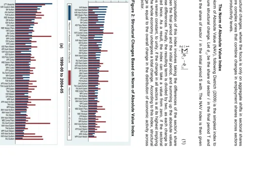
of s truc tur al c hanges , w her e the foc us is onl y on aggr egat e s hi fts in s ec tor al s har es to m o re c o m p le x o n e s th a t co m b in e ch a n g e s in e m p lo y m e n t sh a re s a cr o ss se ct o rs wi th p ro d u c tiv ity le v e ls . 3. 1 The N or m of A bs ol ut e V a lue Inde x Th e N o rm o f A b s o lu te V a lu e ( N A V ), fo llo w in g D ie tri c h ( 2 0 0 9 ) i s th e s im p le s t i n d e x to me a s u re s tru c tu ra l c h a n g e . L e t be the s har e of s ec tor in th e fin a l p e rio d T a n d be the s har e of s ec tor in th e in it ia l p e rio d S wi th . Th e N A V in d e x is th e n g iv e n as

(1

)

Th e c o m p u ta tio n o f th is in d e x in v o lv e s t a k in g t h e d iff e re n c e s o f th e s e c to r’s sh a re bet w een the final per iod and the ini tial per iod , a n d s u m m in g u p th e a b s o lu te v a lu e s of thes e di ffer enc es . F inal ly , the res ul ting ter m is di v ided by tw o, as eac h c hange is co u n te d tw ice . A s a re su lt, th e in d e x ca n ta ke a v a lu e fro m ze ro , if th e se ct o ra l sh a re s re m a in co n st a n t, to u n ity , i f t h e ch a nge in al l s ec tor s is at it s hi ghes t i m pl y ing th a t th e w h o le e c o n o m y u n d e rg o e s a to ta l c h a n g e . A c c o rd in g to th is in d e x , s tr u c tu ra l ch a n g e is e q u a l t o th e o v e ra ll ch a n g e in th e d ist rib u tio n o f e co n o m ic a ct iv ity a cr o ss th e s e c to r. Fi gur e 2 : S tr uc tur a l C ha nge s B a s e d on N or m of A bs ol ut e V a lue Inde x (a ) 1999 -00 to 2004 -05 (b ) 2004 -05 to 2011 -12 So u rc e : Au th o r’s C a lc u la tio n s ! !

φ

i , T

! i

! !

φ

i , S

! i

!

!

2

1

φ

i , T

−

φ

i , S i

∑

0 .05 .1 .15 .2 .25

HAR Western KAR Inland Northern KAR Inland Southern WBE Western Plains UTT Uttaranchal ORI Coastal BIH Central ASS Plains Western ORI Northern HAR Eastern KAR Coastal & Ghats CHH Chhattisgarh TNA Coastal KAR Inland Eastern KER Southern UPR Eastern RAJ Southern MAH Eastern KER Northern MAH Inland Eastern MPR Malwa RAJ South Eastern ASS Plains Eastern APR Inland Northern APR Inland Southern ORI Southern MAH Coastal UPR Southern UPR Central PUN Northern JHA Jharkhand TNA Coastal Northern RAJ North Eastern WBE Central Plains MPR Central BIH Northern MAH Inland Western MAH Inland Central APR Coastal TNA Southern WBE Eastern Plains TNA Inland WBE Himalayan UPR Western PUN Southern MPR Northern MAH Inland Northern RAJ Western APR South Western MPR South MPR Vindhya MPR South Western

N o rm o f Asse t V a lu e (O u tp u t) N o rm o f Asse t V a lu e (Emp lo yme n t)

0 .05 .1 .15 .2 .25

[image:7.612.55.579.96.515.2]

7

Figure 2 highlights these indices for the 52 regions in India. We calculate the indices based on the change in output shares as well as employment shares between 1999-00 and 21999-004-05, and again between 21999-004-05 and 2011-12. The regions are ranked according to extent of structural change observed in terms of output. It is evident that there is very little correlation between change in structure of output and change in structure of employment in both the periods. Thus the change in sectoral share of output in these regions was not accompanied by labour moving in or out of these sectors. For example, in Haryana Western, which experienced the maximum structural change in terms of output, while share of agriculture in district domestic product declined by 11.6 percentage points between 1999-00 and 2004-05, the employment share increased by 0.5 percentage. In several other sectors, including unregistered manufacturing, trade, hotel and restaurants and banking, insurance and real estate, changes in sectoral share of output were in the opposite direction to changes in employment share. On the other hand, although share of registered manufacturing and construction in district domestic product increased by more than 4.0 percentage points, the increase in employment was much more muted.

At the same time, there is a negative, albeit low, correlation between structural changes taking place between 1999-00 and 2004-05 and those taking place between 2004-05 and 2011-12, implying that the process of structural change was not persistent.

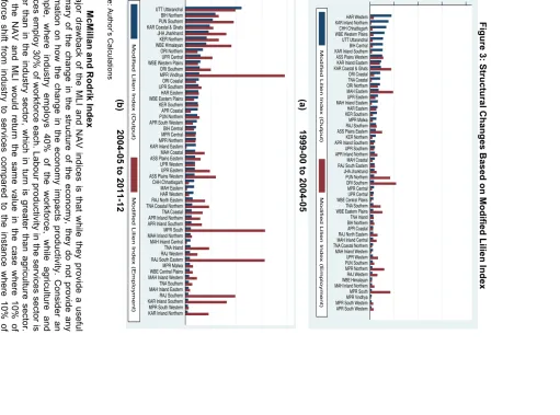
3.2 Modified Lilien Index

The second index used in the literature to measure structural change is a modified Lilien Index. It was originally used to measure the sectoral growth rate for the demand for labour from period S to period T and employed to measure the degree of liquidity of factor reallocation. However, Dietrich (2012) modified the Lilien index by augmenting it with weights of the share of sectors in both periods.

(2)

A low MLI implies that the structural change in the economy is taking place at a slow rate, while a high MLI means that structural change is occurring at a rapid rate. Based on these calculations, we construct the structural change indices for output and employment over the period 1999-00 to 2004-05 and 2004-05 to 2011-12. These are shown in Figure 3.

As can be seen from comparing Figures 2 and 3, the indices developed using the modified Lilien methodology is highly correlated with the indices constructed using the norm of asset value methodology. In fact, for the period 1999-00 to 2004-05, the correlations are as high as 0.93 for output shares and 0.94 for employment shares. While the correlation remains around 0.94 for employment share during the latter period, it increases to 0.96 in the case of output share. Moreover, both MLI and NAV indices indicate that the pace of structural change increased sharply during the period 2004-05 to 2011-12, compared to 1999-00 to 2004-05. While the average structural change in output during the first period according to the NAV and MLI indices were 0.075 and 0.005, respectively, it increased to 0.096 and 0.009 in the second period. Similarly, the average structural change in employment calculated using the NAV and MLI indices rose from 0.071 and 0.005, respectively to 0.114 and 0.017.

!

!

MLI=

φ

_i

,S

φ

i_,T

log

φ

i_,S

φ

i_,T

⎛

⎝

⎜

⎞

⎠

⎟

i

∑

8

Fi gur e 3 : S tr u c tu ra l C h a n g e s B a s e d o n Mo d if ie d L ili e n In d e x (a ) 1999 -00 to 2004 -05 (b ) 2004 -05 to 2011 -12 So u rc e : Au th o r’s C a lc u la tio n s 3. 3 Mc Mi lla n a n d R o d ri k In d e x A m a jo r d ra w b a c k o f th e M L I a n d N AV in d ic e s is t h a t wh ile t h e y p ro v id e a u s e fu l su m m a ry o f th e ch a n g e in t h e st ru ct u re o f th e ec onom y , they do not pr ov ide any in fo rm a tio n o n h o w t h e c h a n g e in t h e ec onom y im pac ts pr oduc tiv ity . Co n s id e r a n ex am pl e, w her e in d u s try e m p lo y s 4 0 % o f th e w o rk fo rc e , w h ile a g ric u lt u re and se rv ice s e m p lo y 3 0 % o f w o rkf o rce e a ch . L a b o u r p ro d u ct iv ity in th e se rv ice s se ct o r i s hi gher t han in the indus try s ec tor , w hi c h in tur n is gr eat er t han agr ic ul tur e s ec tor . Bo th th e N AV a n d M L I w o u ld re tu rn th e s a m e v a lu e in th e c a s e w h e re 1 0 % o f wo rk for c e s hi ft from indus try t o s er v ic es c om par ed to the ins tanc e w her e 10% of wo rk fo rc e s h ift s fr o m in d u s tr y to a g ric u ltu re . H o w e v e r, th e pr oduc tiv ity im pl ic at ions of th e s e tw o m o v e s a re v e ry d iffe re n t w ith la b o u r p ro d u c ti v ity b e in g s ig n ifi c a n tl y hi gher in th e c as e w her e s er v ic es gai n 10% of the w or k for c e, c om par ed to the c as e w her e la b o u r s h if ts to a g ric u lt u re . Th u s a c hange in the s truc tur e of the ec onom y has im por tant im pl ic at ions for labour pr oduc tiv ity , and henc e the ear ni ng pot ent ial and w el far e of the wo rk e rs . To e v a lu a te th e c o n tr ib u ti o n to g ro w th a ris in g fr o m re a llo c a ti o n o f w o rk e rs , th e lite ra tu re

0 .02 .04 .06 .08

HAR Western KAR Inland Northern CHH Chhattisgarh WBE Western Plains UTT Uttaranchal BIH Central KAR Inland Southern ASS Plains Western KAR Inland Eastern KAR Coastal & Ghats ORI Coastal TNA Coastal ORI Northern MAH Eastern UPR Eastern MAH Inland Eastern HAR Eastern KER Southern MPR Malwa RAJ Southern ASS Plains Eastern KER Northern APR Inland Southern UPR Southern APR Inland Northern MAH Coastal RAJ South Eastern JHA Jharkhand PUN Northern ORI Southern MPR Central UPR Central WBE Central Plains TNA Southern WBE Eastern Plains TNA Inland BIH Northern APR Coastal RAJ North Eastern MAH Inland Central TNA Coastal Northern MAH Inland Western UPR Western PUN Southern MPR Northern RAJ Western WBE Himalayan MAH Inland Northern MPR South MPR Vindhya MPR South Western APR South Western

Mo d ifie d L il ie n I n d e x (O u tp u t) Mo d ifie d L il ie n I n d e x (Emp lo yme n t)

0 .02 .04 .06 .08

UTT Uttaranchal BIH Northern PUN Southern KAR Coastal & Ghats JHA Jharkhand KER Northern WBE Himalayan ORI Northern UPR Central WBE Western Plains ORI Southern MPR Vindhya ORI Coastal UPR Southern HAR Eastern WBE Eastern Plains KER Southern APR Coastal PUN Northern APR South Western BIH Central MPR Central MPR Northern KAR Inland Eastern MAH Coastal ASS Plains Eastern UPR Western UPR Eastern ASS Plains Western CHH Chhattisgarh MAH Eastern HAR Western RAJ North Eastern TNA Coastal Northern TNA Coastal APR Inland Northern APR Inland Southern MPR South MAH Inland Northern MAH Inland Central TNA Inland RAJ Western RAJ South Eastern MPR Malwa WBE Central Plains MAH Inland Western TNA Southern MAH Inland Eastern RAJ Southern KAR Inland Southern MPR South Western KAR Inland Northern

[image:9.612.101.693.95.520.2]

9

decomposes the change in labour productivity into ‘within effect’ and ‘reallocation effect’. While the within effect captures productivity growth within sectors, the reallocation effect or structural change measures the productivity effect of reallocation of labour among the different sectors. De Vries et al. (2015) point out that this decomposition can be performed in various ways depending on the choice of the base and the end years of the periods, which has important implications for the measurement and interpretation of structural change.

McMillan and Rodrik (2011) consider the base period employment shares and final period productivity levels. More specifically, the change in labour productivity is decomposed as

(3)

where is the change in aggregate labour productivity between final and initial

period, and and are the sectoral labour productivity levels in the final and

initial period, respectively. Similarly, and are the final and initial employment

shares of the various sectors. The first term is positive when the weighted change in labour productivity levels in sectors is positive, and reflects the contribution to overall productivity change from an increase in sectoral labour productivity. This is referred to as the within effect. The second term in Equation 3 is the reallocation effect, which reflects the change in labour productivity due to reallocation of employment across sectors, and is positive when labour moves from less to more productive sectors. This is also referred to as structural change in McMillan and Rodrik (2011) and Hasan et al. (2015).

Figure 4 decomposes average annual growth in labour productivity into average annual growth in within effect and average annual growth in reallocation effect. The regions are ranked according to average annual growth in reallocation effect. At the aggregate level, the growth in average annual labour productivity was 3.16% during 1999-00 to 2004-05, of which 1.52% was due to within effect and 1.64% was a result of reallocation effect. In the subsequent period, growth in average annual labour productivity more than doubled to 8.06%, with a significant part of the increase coming from growth of within effect, which jumped to 6.15%. Average annual growth in the reallocation effect witnessed a small increase, rising up to 1.91%. However, the aggregate growth in productivity levels masks a lot of variation at the regional level.

!

!

Δ

Y

=

(

y

_i,T

−

y

_i,S

)

i

∑

φ

_i,S

+

(

φ

_i,T

−

φ

_i,S

)

i

∑

y

_i,T

!

Δ

Y

!

!

y

i,T

!

!

y

i,S

!

10

Fi gur e 4 : D e c om pos it ion of P roduc tivi ty G row th (a ) 1999 -00 to 2004 -05 (b ) 2004 -05 to 2011 -12 So u rc e : Au th o r’s C a lc u la tio n s Th e p e rio d b e tw e e n 1 9 9 9 -00 and 2004 -05 ex per ienc ed a lot of v ol at ilit y , w ith 29 re g io n s w itn e s s in g ei ther a negat iv e gr ow th in w ithi n ef fec t or a negat iv e gr ow th in re a llo c a tio n e ffe c t, w h ile in o n e re g io n b o th g ro w th ra te s w e re n e g a ti v e . T h e re m a in in g re g io n s w it n e s s e d a n in c re a s e in ‘w it h in e ffe c t’ a s w e ll a s ‘r e a llo c a tio n ef fec t’. Th e s e c o n d p e rio d is re la tiv e ly m o re h o m o g e n o u s w ith a ll th e re g io n s wi tn e s s in g p o s itiv e g ro wt h in wi th in e ffe c t, a lth o u g h 15 re g io n s s till re c o rd e d n e g a tiv e st ru ct u ra l ch a n g e g ro w th .

-10 -5 0 5 10 15

ORI Southern MAH Eastern KAR Coastal & Ghats MAH Inland Central WBE Eastern Plains CHH Chhattisgarh ORI Northern MAH Inland Northern WBE Western Plains MPR South Western TNA Coastal Northern MPR Northern TNA Inland KAR Inland Eastern TNA Southern BIH Central APR Coastal MPR South MAH Inland Eastern HAR Eastern RAJ North Eastern MAH Coastal MAH Inland Western RAJ Western KER Northern MPR Vindhya WBE Central Plains TNA Coastal HAR Western APR Inland Northern RAJ Southern JHA Jharkhand ORI Coastal MPR Central MPR Malwa KAR Inland Northern UPR Western UPR Central UPR Eastern KER Southern PUN Northern PUN Southern UTT Uttaranchal BIH Northern WBE Himalayan APR South Western APR Inland Southern KAR Inland Southern UPR Southern ASS Plains Western RAJ South Eastern ASS Plains Eastern

An n u a l G ro w th in R e a llo ca tio n Ef fe ct An n u a l G ro w th in W it h in Ef fe ct

-10 0 10 20

[image:11.612.125.702.93.516.2]

11

3.4 De Vries, Timmer and De Vries Index

De Vries et al (2015) argue that the structural change term in the McMillan and Rodrik index is only a static measure of the reallocation effect as it depends on the differences in productivity level and not their growth rates. Absorption of additional workers in a high productivity sector can result in depressing productivity growth as the marginal productivity of these additional workers might be low. To account for this De Vries et al. (2015) suggest an alternative decomposition method that accounts for the possibility that growth and levels across the sectors are negatively correlated. It uses the base periods for the productivity levels as well as employment share, and introduces a third interaction term.

(4)

Here, the first term as before reflects the contribution to overall productivity change from an increase in sectoral labour productivity (the ‘within effect’). In the second term, the term within parenthesis would be positive for sectors that have witnessed an increase in employment share and negative for sectors that have experienced a decline in employment share. So, a positive second term would imply that sectors, which witnessed an increase in employment share, were the ones that had a higher level of initial productivity. The third term, which is the interaction term, represents the joint effect of changes in sectoral productivity levels and employment shares. A positive term implies that workers are moving into sectors where productivity levels are increasing.

Thus the reallocation effect term in Equation (3) is broken into two different terms in Equation (4) where the first term represents if labour has moved into sectors that have above average productivity levels and the second term indicates if sectors that have witnessed an increase in employment shares have also experienced productivity growth. De Vries et al (2015) refer to the first term as ‘static reallocation effect’ and the second term as ‘dynamic reallocation effect’.

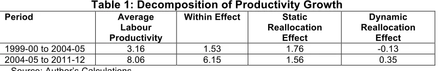
[image:12.612.94.522.615.685.2]

The productivity decomposition at the aggregate level among the three effects is illustrated in Table 1. The ‘within effect’ is same as in Section 3.3, while the structural change term is broken down into ‘static reallocation effect’ and ‘dynamic reallocation effect’. While the former is positive in both the periods implying that workers did move into above average productivity sectors, the latter is positive only in the second period, indicating that workers moved into sectors that were witnessing labour productivity growth.

Table 1: Decomposition of Productivity Growth

Period Average

Labour Productivity

Within Effect Static

Reallocation Effect

Dynamic Reallocation

Effect

1999-00 to 2004-05 3.16 1.53 1.76 -0.13

2004-05 to 2011-12 8.06 6.15 1.56 0.35

Source: Author’s Calculations

Again, as before, the aggregate picture masks a great deal of heterogeneity. Figure 5 illustrates the decomposition of labour productivity growth across the different regions during the two time periods. The regions are ranked according to the dynamic reallocation effect. As is evident, during the period 1999-00 to 2004-05, in only six regions out of 52, labour moved into sectors that experienced productivity

!

!

ΔY

=

(

y

_i,T

−

y

_i,S

)

i

∑

φ

_i,S

+

(

φ

_i,T

−

φ

_i,S

)

i

∑

y

_i,S

+

(

y

_i,T

−

y

_i,S

)

(

φ

_i,T

−

φ

_i,S

)

12

gr ow th or m ov ed ou t o f s e c to rs th a t e x p e rie n c e s d e c lin e in p ro d u c ti v ity . En c o u ra g in g ly , in th e s e c o n d p e rio d , th e n u m b e r o f re g io n s w itn e s s in g p o s iti v e dy nam ic r eal loc at ion ef fec t m or e than doubl ed to four teen . Ev e n in th e c a s e o f s ta tic re a llo c a tio n ef fec t, the num ber of regi ons ex per ienc ing pos itiv e gr ow th inc reas ed si g n ifica n tly fr o m th e fi rs t p e rio d to th e s e c o n d , im p ly in g th a t in m o re re g io n s w o rk e rs we re m o v in g to s e c to rs c h a ra c te riz e d b y a b o v e a v e ra g e p ro d u c tiv ity . Fi gur e 5 : P ro d u c tiv it y D e c o m p o s it io n A c ro s s t h e Re g io n s ( 1 9 9 9 -2011) (a ) 1999 -00 to 2004 -05 (b ) 2004 -05 to 2011 -12 So u rc e : Au th o r’s C a lc u la tio n s

-20 -10 0 10 20

KER Northern MAH Coastal KAR Inland Northern TNA Southern TNA Coastal WBE Central Plains PUN Southern KER Southern MPR Central APR Coastal WBE Himalayan MAH Inland Western APR Inland Northern RAJ North Eastern TNA Coastal Northern UPR Western MPR Vindhya UPR Eastern APR South Western RAJ Southern TNA Inland WBE Western Plains ORI Northern PUN Northern KAR Inland Southern UPR Central HAR Eastern BIH Northern MAH Inland Northern APR Inland Southern UTT Uttaranchal CHH Chhattisgarh ORI Coastal KAR Inland Eastern JHA Jharkhand UPR Southern HAR Western MAH Inland Eastern RAJ Western MPR South WBE Eastern Plains ASS Plains Western MPR Malwa BIH Central MAH Inland Central MAH Eastern RAJ South Eastern KAR Coastal & Ghats MPR South Western ORI Southern MPR Northern An n u a l G ro w th in W ith in Ef fe ct An n u a l G ro w th in St a tic R e a llo ca tio n Ef fe ct An n u a l G ro w th in D yn a mi c R e a llo ca tio n Ef fe ct

-10 0 10 20 30

[image:13.612.49.699.127.520.2]

13

4.

Impact of Structural Change on Reduction in Poverty across

Regions

[image:14.612.98.513.281.539.2]

In this section, we consider the experience of regions with regards to poverty reduction. Again, as can be seen in Figure 6 below, 9 regions witnessed an increase in poverty, while the remaining regions experienced a drop in poverty. More importantly, the extent of change varied considerably across the regions. Regions from the southern states witnessed some of the fastest reduction in poverty with 9 out of the top 10 regions in terms of poverty reduction belonging to these states. This is in line with Hasan et al (2015), which also points out that southern states of Kerala, Tamil Nadu, Karnataka and Andhra Pradesh witnessed the highest poverty reduction between 1987 and 2009. The evidence at the other end is more varied. While Maharashtra and Karnataka had two regions each that witnessed an increase in poverty, the states of Andhra Pradesh, Punjab, Madhya Pradesh, West Bengal and Uttar Pradesh reported one such region each.

Figure 6: Average Annual Rate of Poverty Reduction across Regions (1999-00 to 2011-12)

Source: Author’s Calculations

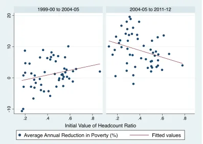
We also investigate if regions are exhibiting a convergence in terms of poverty rates. For this to happen, poverty reduction needs to occur at a faster pace in regions where initial poverty rates are high. Figure 7 provides a relationship between average annual rate of poverty reduction and initial poverty rates during the periods 1999-00 to 2004-05 and 2004-05 to 2011-12. While the first period witnessed some degree of convergence with a positive relationship between the two variables, the trend reverses in the subsequent period with regions exhibiting lower poverty rates in 2004-05 witnessing faster reduction in poverty between 2004-05 and 2011-12.

Next, we focus on the relationship between the various measures of structural change and poverty reduction. We evaluate the impact of the different measures of structural change on poverty reduction using a simple regression specification outlined as (5) -2 0 -1 0 0 10 20 APR In la nd N ort he rn TNA Inland APR In la nd So ut he rn T N A C oa st al KER N ort he rn APR C oa st al R AJ N ort h Ea st ern KER So ut he rn T N A C oa st al N ort he rn APR So ut h W est ern U T T U tta ra nch al MAH In la nd C en tra l PU N So ut he rn KAR In la nd Ea st ern MPR Ma lw a O R I C oa st al MAH C oa st al W BE C en tra l Pl ai ns MAH In la nd Ea st ern R AJ W est ern H AR Ea st ern R AJ So ut h Ea st ern W BE Ea st ern Pl ai ns ASS Pl ai ns W est ern BI H N ort he rn W BE W est ern Pl ai ns U PR W est ern O R I N ort he rn BI H C en tra l ASS H ill s O R I So ut he rn U PR Ea st ern JH A Jh arkh an d H AR W est ern C H H C hh at tisg arh MPR N ort he rn U PR So ut he rn MPR So ut h W est ern MPR So ut h T N A So ut he rn MPR V in dh ya ASS Pl ai ns Ea st ern R AJ So ut he rn KAR C oa st al & G ha ts W BE H ima la ya n KAR In la nd So ut he rn MAH Ea st ern MAH In la nd W est ern U PR C en tra l KAR In la nd N ort he rn MAH In la nd N ort he rn MPR C en tra l PU N N ort he rn

!

14

where is the average annual rate of poverty reduction between period and

in region and is the poverty rate in region in the initial period i.e.

and is the main variable of interest. It takes the value of the NAV and MLI

[image:15.612.100.497.216.498.2]

index when structural change is measured by these indices, and the average annual rate of growth rate of labour productivity and its components ‘within effect’ and ‘reallocation effect’ when productivity growth is decomposed into these effects.

Figure 7: Relationship between Average Annual Rate of Poverty Reduction and Initial Poverty Rate (1999-00 to 2011-12)

Source: Author’s Calculations

The inclusion of lagged poverty rate serves two purposes. First, it captures the potential for poverty reduction in a region, as a larger initial poverty rate implies that more people can be pulled out of poverty. Second, it also provides a sense of whether poverty rates are converging across the regions or diverging. A positive and

significant implies that regions with high poverty rates have witnessed faster

poverty reduction, as a result of which poverty rates across the regions would be converging.

The NAV and MLI indexes summarize the overall change in the distribution of economic activity across the different sectors of the region. Below, we report the results of the regression analysis using these indexes for the period 1999-00 to 2011-12. The first two specifications in columns (I) and (II) are panel estimations with fixed effects, controlling for heteroskedasticity and within panel serial correlation in the idiosyncratic error term . To evaluate the robustness of the results we also

estimate Equation (5) using generalized least square methodology, again controlling for heteroskedasticity and autocorrelation within panels. The results are outlined in columns (III) and (IV).

!

!

Y

j,t,t−s

!t

!t

−

s

!j

!

!

X

j,t−s

!j

!t

−

s

!

!

Z

j,t,t−s

-1

0

0

10

20

.2 .4 .6 .8 .2 .4 .6 .8

1999-00 to 2004-05 2004-05 to 2011-12

Average Annual Reduction in Poverty (%) Fitted values

Initial Value of Headcount Ratio

β

[image:16.612.127.484.106.267.2]

15

Table 2: Effect of Structural Change Indexes on Poverty Reduction

Fixed Effects Generalized Least Squares

I II III IV

Constant 1.820 5.857*** -17.990** -11.556*

[1.362] [9.597] [-2.504] [-1.693] Lagged Poverty Rates -5.906*** -4.833*** 33.385** 33.086**

[-2.855] [-6.354] [2.160] [2.056]

Structural Change (NAV) 63.047*** 109.566***

[6.022] [3.671]

Structural Change (MLI) 146.908*** 434.847***

[3.247] [3.171]

Observations 104 104 104 104

Number of Regions 52 52 52 52

Note: t-statistics in brackets, *** p<0.01, ** p<0.05, * p<0.1 Source: Author’s Calculations

It is evident that structural change, as measured by the NAV and MLI indexes, has contributed in a significant manner to reduce poverty, after controlling for initial poverty rates. This result is robust across fixed effects and generalized least squares panel estimations. Thus, the change in the structure of production between 1999-00 and 2011-12 was poverty reducing in the case of India. However, given that NAV and MLI indexes are agnostic about the relationship between structural change and productivity it is not possible to chart out the manner in which structural change, as reflected by these two indices, has brought about a decline in poverty.

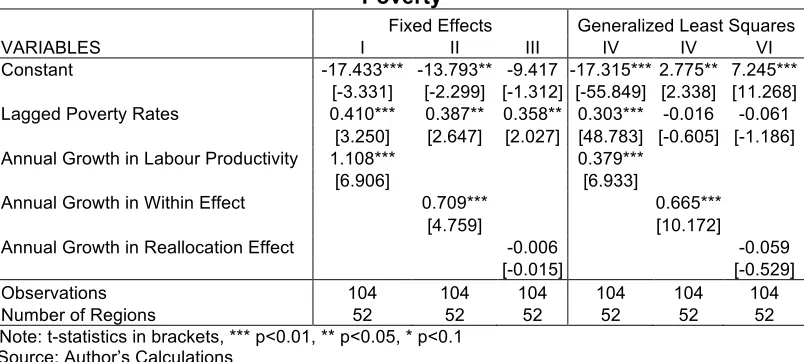
[image:16.612.105.507.527.708.2]

To overcome this difficulty, we use the measure outlined in Equation (3), which focuses on productivity growth. With productivity being positively correlated to average wages across sectors, an increase in productivity is likely to result in a drop in poverty by raising the earning potential of the individual. Equation (3) decomposes aggregate productivity into the within and reallocation effects, with the latter being dubbed as structural change in McMillan and Rodrik (2013) and Hasan et al. (2015). We evaluate the impact of aggregate labour productivity growth as well as its components—within and reallocation effects—on poverty reduction in Table 3.

Table 3: Impact of Aggregate Productivity Growth and Its Components on Poverty

Fixed Effects Generalized Least Squares

VARIABLES I II III IV IV VI

Constant -17.433*** -13.793** -9.417 -17.315*** 2.775** 7.245***

[-3.331] [-2.299] [-1.312] [-55.849] [2.338] [11.268] Lagged Poverty Rates 0.410*** 0.387** 0.358** 0.303*** -0.016 -0.061

[3.250] [2.647] [2.027] [48.783] [-0.605] [-1.186]

Annual Growth in Labour Productivity 1.108*** 0.379***

[6.906] [6.933]

Annual Growth in Within Effect 0.709*** 0.665***

[4.759] [10.172]

Annual Growth in Reallocation Effect -0.006 -0.059

[-0.015] [-0.529]

Observations 104 104 104 104 104 104

Number of Regions 52 52 52 52 52 52

Note: t-statistics in brackets, *** p<0.01, ** p<0.05, * p<0.1 Source: Author’s Calculations

16

poverty reduction, similar to the findings in Hasan et al. (2015). However, we find that annual growth in reallocation effect or structural change has no significant impact on poverty reduction. This is in sharp contrast to the findings of Hasan et al, which finds that the reallocation effect has a strong positive impact on poverty reduction. One plausible reason for the different results could be the use of different samples. While Hasan et al focus on 18 major states, and cover the period 1987 to 2009-10 we cover the period from 1999-00 to 2011-12, and conduct the analysis at a sub-state level.

[image:17.612.98.530.272.514.2]

To delve deeper into the impact of reallocation effect on poverty reduction, we make use of the decomposition outlined in Equation (4) where reallocation effect or the structural change is further broken down into static reallocation effect and dynamic reallocation effect. The results are outlined in Table 4 below.

Table 4: Impact of Aggregate Productivity Growth and Its Components on Poverty

Fixed Effects Generalized Least Squares

VARIABLES I II III IV V VI VII VIII

Constant -17.433*** -13.793** -6.881 -4.347 -17.315*** 2.775** -1.087*** 6.284*** [-3.331] [-2.299] [-0.966] [-0.630] [-55.849] [2.338] [-2.720] [15.306] Lagged Poverty Rates 0.410*** 0.387** 0.329* 0.292* 0.303*** -0.016 0.098*** -0.020*** [3.250] [2.647] [1.907] [1.760] [48.783] [-0.605] [12.888] [-2.905]

Annual Growth in Labour 1.108*** 0.379***

Productivity [6.906] [6.933]

Annual Growth in Within 0.709*** 0.665***

Effect [4.759] [10.172]

Annual Growth in Static -0.487 -0.456

Reallocation Effect [-1.499] [-1.541]

Annual Growth in Dynamic 1.217*** 0.727***

Reallocation Effect [2.801] [24.864]

Observations 104 104 104 104 104 104 104 104

Number of Regions 52 52 52 52 52 52 52 52

Note: t-statistics in brackets, *** p<0.01, ** p<0.05, * p<0.1 Source: Author’s Calculations

Columns (I), (II), (V) and (VI) replicate the results outlined in Table 4 as it tests the same specification outlined there. Columns (III) and (VII) indicate that annual growth rate of static reallocation has an insignificant impact on poverty reduction under both specifications, thereby implying that movement of workers to above average productivity level sectors in the initial period is not poverty reducing. In sharp contrast, we find from Columns (IV) and (VIII) that the annual growth in dynamic reallocation effect has a strong positive impact on poverty reduction. Thus as employment shares of sectors that are witnessing a productivity growth increases, it leads to a reduction in poverty reduction. Moreover, the coefficient on dynamic reallocation effect is considerably higher than the coefficients on either aggregate labour productivity or other two components i.e. within effect and static reallocation effect. Thus, reallocation of workers to sectors, which are experiencing an increase in productivity or reallocation of workers out of sectors where the productivity is slowing down is a vital channel for poverty reduction.

17

With a view to help our understanding of how various components of labour productivity is influencing poverty rates in India, we aggregate the six regions which recorded the highest average annual decline in poverty and compare it with the aggregate of six regions with lowest poverty reduction. The results are outlined in Figure 8. The sectors are based on (ascending) order of sectoral productivity in 2011-12.

A common factor across the two sets of regions is the agricultural sector, which was the biggest source of employment, experiencing positive growth in sectoral labour productivity i.e. within effect, but negative growth in both static and dynamic reallocation effects. This implies that for poverty reduction to occur at an accelerated pace, improving labour productivity in the agriculture sector and pulling people out of agriculture is not enough. The pace of poverty reduction crucially depends on sectors that are absorbing the workers coming out of agriculture. Moreover, in both sets of regions, a small fraction of the labour is reallocated to unregistered manufacturing, which was the second least productive sectors in both these set of regions.

[image:18.612.114.500.409.667.2]

While construction, which was the third least productive sector in both regions, witnessed a strong increase in employment share in the low poverty reducing regions, it also experienced a decline in sectoral productivity resulting in a negative dynamic reallocation effect. In contrast, the high poverty reducing regions witnessed a positive dynamic reallocation on account of an increase in employment share as well as improvement in labour productivity.

Figure 8: Productivity Growth Decomposition by State and Sector (1999-00 to 2011-12)

Note: The sectors are defined as follows: A = Agriculture and Allied Activities; B = Registered Manufacturing; C = Unregistered Manufacturing; D = Construction; E = Trade, Hotel and Restaurants; F = Transport, Storage and Communications; G = Finance, Insurance and Real Estate; H: Public Administration; and I = Community, Social and Personal Services

Source: Author’s Calculations

Focusing on the remaining sectors the following salient features stand out. In the high poverty reducing regions, all the top six sectors in terms of sectoral productivity,

-.

5

0

.5

1

1.

5

A C D I E H F B G A C D I E F H B G

High Poverty Reducing Regions Low Poverty Reducing Regions

Sectoral Growth in Within Effect Sectoral Growth in Static Reallocation

Sectoral Growth in Dynamic Reallocation

Pe

rce

n

t(%

)

18

witnessed an improvement in labour productivity, along with an increase in employment share resulting in positive dynamic reallocation affect. In particular, the increase was substantial in the case of registered manufacturing, transport, storage and communication and banking, insurance and real estate, the three highest productive sectors in 2011-12. Thus these regions were able to generate jobs in modern dynamic sectors, which at the same time were recording strong increases in labour productivity.

Contrast this with the performance of the low poverty reducing regions. Among the high productivity sectors only registered manufacturing and finance, insurance, and real estate sectors witnessed an increase in employment share. Of these, in the case of registered manufacturing, there was very little improvement in productivity, resulting in the dynamic reallocation effect of the sector being a fraction of that in the high poverty reducing region. While the other high productivity sectors viz. trade, hotel and restaurant, public administration and transport, storage and communication witnessed an increase in labour productivity, they experienced a decline in the share of employment and consequently recorded a negative dynamic reallocation effect.

5.

Summary and Conclusions

The main task of this research has been to quantify the nature and extent of the structural changes that have accompanied economic growth since 1999-00 and analyze its implications for poverty reduction in India at the sub-state level. Based on the availability of data, the research focuses on 9 sectors across 52 regions in the 18 larger states; two sub-periods 1999-00 to 2004-05 and 2004-05 to 2011-12. The main findings of the paper are outlined below.

First, as one would expect, average productivity grew at an average annual rate of 3.2% during the first period and accelerated sharply to 8.1% during the second period in line with GDP growth4. Average productivity grew for all regions and there is evidence to suggest that there was some degree of convergence among the 52 regions between 1999-00 and 2011-12.

Second, as revealed by aggregate measures of structural change of the economy such as NAV and MLI, both in terms of output as well as employment, it is clear that the quantum of change was greater in the second period as compared to the first period. There is also evidence to suggest that process of structural change was not persistent across the two periods. But, more importantly, low correlation between the change in the structure of output and that of employment means that movement of labor across sectors did not accompany the change in output.

Third, decomposition of growth in productivity reveals that the ‘within effect’ dominates the ‘reallocation effect’, accounting for most of the increase in productivity for a majority of the regions as well as at the aggregate level. The ‘reallocation effect’ is positive for India at the aggregate level for both periods, but the ‘dynamic reallocation effect’ if positive only in the second period. It is also significant that the extent of domination of the within effect is much more pronounced in the second period when productivity growth was much larger in comparison.

19

Fourth, there is significant positive impact of structural transformation of the economy on poverty reduction between 1999-00 and 2011-12. This holds for aggregate measures (NAV and MLI) as well as for decompositions of productivity growth in the form of ‘within effect’ and ‘dynamic reallocation effect’. At the same time, the impact is not significant in the case of ‘reallocation effect’ in its aggregate form and its component ‘static reallocation effect’.

In conclusion, this paper documents the key dimensions of structural change that has taken place in the Indian economy since 1999-00. While there is little doubt that structural transformation has been poverty reducing in India, the paper raises important questions about the channels though which this impact has been generated, which has important implications both for policy making and future research.

Given the significant impact of the ‘within effect’ in poverty reduction, it is important to understand the scope for further increasing the productivity levels of the low productivity sectors themselves. This is important as India’s productivity levels in sectors such as agriculture, construction and unregistered manufacturing are far below several of its developing counterparts. In this context, the point where reallocation effect will become more important than within effect in terms of its contribution to productivity growth needs to be better understood. An assessment of the situation will allow framing better policy inputs for improving welfare of people engaged in the low productive sectors.

While the situation varies among regions, the ‘reallocation effect’ is positive in aggregate, meaning labor has moved to more productive sectors. Moreover, the ‘dynamic reallocation effect’ component, which is positively related with poverty reduction, is positive in the second period. So, another hypothesis which needs to be tested is the importance of high growth in inducing positive dynamic reallocation effect. This is especially important as the dynamic reallocation effect is positive for a small proportion of regions — six in the first period and 14 in the second.

20

References

Besley, T., and R. Burgess (2000) “Land Reform, Poverty Reduction and Growth:

Evidence from India”, The Quarterly Journal of Economics, Vol. 117 (4), pages 389- 430.

Botero, J., S. Djankov, R. La Porta, F. Lopez-Di Silanes, and A. Shleifer (2004) “The

Regulation of Labor”, The Quarterly Journal of Economics, Vol. 119 (4), pages 1339–1382.

Betts, C., R. Giri, and R. Verma (2013) “Trade, Reform, and Structural Transformation in South Korea”, CAFE Research Paper no.13.03.

Chenery, H. B. (1960) “Patterns of Industrial Growth”, American Economic Review. Vol. 50 (4), pages 624–654.

Dekle, R., and G. Vandenbroucke (2012) “A quantitative analysis of China's structural transformation”, Journal of Economic Dynamics and Control, Vol. 36(1), pages 119-135.

De Vries, G., T. Marcel and K. de Vries, (2015) "Structural Transformation in Africa: Static Gains, Dynamic Losses," Journal of Development Studies, Vol. 51(6), pages 674-688.

Dietrich, A. (2012) "Does Growth Cause Structural Change, or is it the Other Way

Around? A Dynamic Panel Data Analysis for Seven OECD Countries," Empirical

Economics, Vol. 43(3), pages 915-944.

Fallon, P. R., and R. E. B. Lucas (1993) “Job Security Regulations and the Dynamic

Demand for Industrial Labor in India and Zimbabwe”, Journal of Development Economics,

Vol.40 (2), pages 241–75.

Felipe, J., C. Dacuycuy, and M. Lanzafame (2014) “The Declining Share of Agricultural Employment in the People’s Republic of China”, ADB Economics Working Paper Series No. 419.

Felipe, J., A. Mehta, and C. Rhee (2015) “Manufacturing Matters...but It’s the Jobs that

Count”, ADB Economics Working Paper Series No. 420.

Hasan, R., S. Lamba, and A. Sen Gupta (2015) “Growth, Structural Change and Poverty Reduction”, in K.V. Ramaswamy eds., Labour, Employment and Economic Growth in India, Cambridge University Press, pages 91-126

Kochhar, K., U. Kumar, R. Rajan, A. Subramanian, and I. Tokatlidis (2006) “India's

pattern of development: What happened, what follows?” Journal of Monetary

Economics, Vol. 53(5), pages 981-1019.

Kuznets, S. (1971) “Economic Growth of Nations: Total Output and Production Structure”, Belknap Press of Harvard University Press.

Lin, J. Y., and C. Monga (2010) “Growth Identification and Facilitation: The Role of the State in the Dynamics of Structural Change”, World Bank Policy Working Paper No. 5313.

21

Sustainable, International Labor Organization and World Trade Organization, Geneva, pages 49-84

McGregor, N. and B. Verspagen (2016) “The Role of Structural Transformation in the Potential of Asian Economic Growth”, ADB Economics Working Paper Series No. 479.

McMillan, M., D. Rodrik, and I. Verduzci-Gallo (2014) “Globalization, Structural Change, and Productivity Growth, with an Update on Africa”, World Development, Vol. 63 (1), pages 11–32.

Sen, K., and R. Vaidya (1997) “The Process of Financial Liberalization in India”,Oxford

University Press, Delhi.

Sen, K. (2009) “Trade Policy, Inequality and Performance in Indian Manufacturing”,

London: Routledge.

Sen, K. (2014) “The Indian Economy in the Post-Reform Period: Growth without Structural Transformation?”, In D. Davin and B. Harriss-White, eds. China and India:

Pathways of Economic and Social Development,Oxford University Press.

Sen, K. (2016) “The Determinants of Structural Transformation in Asia: A Review of the Literature”, ADB Economics Working Paper Series no. 478.

Stiglitz, J., and A. Weiss (1981) “Credit Rationing in Markets with Imperfect Information”

American Economic Review, Vol.71 (3), pages 393–410.

Studwell, J. (2013) “How Asia Works: Success and Failure in the World’s Most Dynamic

Region”, London: Profile Books.

Ungör, M. (2015) “Productivity Growth and Labor Reallocation: Latin America Versus East Asia”, Manuscript, Central Bank of Turkey, Istanbul.

Teignier, M. (2013) “The Role of Trade in Structural Transformation”, University of Barcelona Working Paper No. E13/300.

Verma, R. (2012) “Can Total Factor Productivity Explain Value Added Growth in

Services?”, Journal of Development Economics, 99(1), pages 163-177.