Munich Personal RePEc Archive
Bubbles, Bluffs, and Greed
Harashima, Taiji
Kanazawa Seiryo University
15 May 2015
Online at
https://mpra.ub.uni-muenchen.de/64361/
Bubbles, Bluffs, and Greed
Taiji Harashima
*May 2015
Abstract
A rational bubble cannot theoretically exist if people have infinite horizons. This paper shows that a bubble-like phenomenon can be generated by a “bluff” even if people are rational and have infinite horizons. A bluff is defined as the behavior of an agent who pretends to possess private information to gain profits, particularly (false or misleading) information that the
representative household’s rate of time preference (RTP RH) has changed. An alternative
definition of the representative household indicates that households must ex ante generate an expected RTP RH to behave optimally, but the expected RTP RH has to be generated based on beliefs about the RTP RH. Bluffers exploit the opportunities derived from the fragile nature of the expected RTP RH. The driving force behind bluffs is greed because bluffers do not work hard to gain profits by producing and selling better goods and services more cheaply, but by disseminating contaminated information, or acting in such a way to mislead people into believing the expected RTP RH has changed.
JEL Classification code: E32, E44, G14
Keywords: Bubble; Bluff; Greed; Time preference; The representative household; The financial supervision
*Correspondence: Taiji HARASHIMA, Kanazawa Seiryo University, 10-1 Goshomachi-Ushi, Kanazawa-shi, Ishikawa, 920-8620, Japan.
1 INTRODUCTION
The Great Recession that occurred in the latter half of the 2000s forced us to once again realize
the importance of the economic phenomenon known as a “bubble”. In this case, it was not only a single commodity’s bubble that burst but a global bubble-led economic boom. Theoretically, a
rational bubble cannot exist if agents have infinite horizons (Blanchard and Watson, 1982; Santos and Woodford, 1997). Hence, an economic boom led by a rational bubble is also impossible if agents have infinite horizons. An assumption of some kind of irrationality may
therefore be necessary to explain the existence of bubble-like phenomena. However, merely making ad hoc assumptions of irrational agents does not appear to be a compelling argument. It is too easy to ad hoc assume irrationality because, if we assume irrationality in human behaviors, we can explain any otherwise unexplainable human phenomena. However, there is another
possible source of this bubble-like phenomenon. If some factor or factors obstruct agents’ rational decision making, a bubble may be generated. In this paper, I show that a mechanism
which I call a “bluff” is such a factor, and it generates a bubble-like phenomenon even if people are rational and have infinite horizons. In this context, I consider a bluff to be a strategy or trick
in which an agent pretends to possess private information that is actually untrue to gain profit. To the best of my knowledge, this type of strategy has not been studied as a source of
bubble-like phenomena, but it can potentially obstruct agents’ decision making and force them to make non-optimal decisions ex post; in other words, people can potentially be fooled or cheated by an agent who bluffs.
I show that, by utilizing private information about the rate of time preference of the representative household (RTP RH), a bluffer can generate a bubble-like phenomenon. Becker
(1980) and Harashima (2014a, b) indicate that it is not possible to assume the representative household as the average household in dynamic models. An alternative definition of the
representative household is shown in Harashima (2014a, b); it entails the collective behavior of households under sustainable heterogeneity. This alternative definition of the representative
household requires that each household must generate an expected RTP RH ex ante for it to behave optimally. However, although a household knows its own rate of time preference (RTP),
it cannot directly observe the RTP RH. Therefore, the expected RTP RH has to be generated based on each household’s beliefs about the RTP RH. The expected RTP RH is therefore fragile.
If bluffers can exploit opportunities provided by this fragility and manipulate the expected RTP RH, the use of bluffs can cause a bubble-like phenomenon.
greed. However, some people have argued that greed is an indispensable driving force of
capitalism and therefore should not be blamed. Bluffers’ greed, however, should clearly be blamed for negative economic outcomes because bluffers do not work harder to obtain profits
by producing and selling better goods and services more cheaply; rather, they gain profit by acting in such a way to mislead people into believing the expected RTP RH has changed.
2 THE EXPECTED RTP RH
2.1 An alternative definition of the representative household
2.1.1 The definition
As Becker (1980) and Harashima (2014a, b) indicate, it is not possible to assume the representative household as the average household in dynamic models. Harashima (2014a, b)
shows an alternative definition of the representative household such that the behavior of the representative household is defined as the collective behavior of all households under sustainable heterogeneity. The reason why this alternative definition is needed and the nature of
sustainable heterogeneity are described in detail in the Appendix. Unlike the case in which the representative household is assumed to be the average household, this alternatively defined
representative household reaches a steady state in which all households satisfy all of their optimality conditions in dynamic models, even if households are heterogeneous. In addition, the
alternatively defined representative household has an RTP that is equal to the average RTP as shown in equations (A7) and (A8) in the Appendix.1 Hence, we can assume not only a
representative household but also that its RTP is the average rate of all households.
2.1.2 Necessity of expecting RTP RH
This alternatively defined representative household requires that each household must generate
an expected RTP RH exante for it to behave optimally as shown in the Appendix (see also Harashima, 2014a, b). However, a problem remains. Although a household knows its own RTP,
it cannot directly observe the RTP RH, and therefore, the expected RTP RH has to be generated based on its beliefs about RTP RH. Beliefs will be formed by using heuristics (a detailed explanation of the expected RTP RH and the heuristics used to estimate it are shown in the
Appendix).
1 If sustainable heterogeneity is achieved with the help of government intervention, the time preference
2.2 The path when the expected and intrinsic RTP RHs are
different
The alternative definition of the representative household requires sustainable heterogeneity. Achieving sustainable heterogeneity affects the behavior of individual households because
sustainable heterogeneity requires that each household must consider other households’ optimality (as well as the behavior of the government, if necessary). This feature does not,
however, mean that households behave cooperatively. Each household behaves autonomously based on its own RTP, but at the same time, its behavior is influenced by whether or not the
other households’ optimality conditions are achieved. This consideration affects the actions a
household takes in that it affects the choice of a household’s initial consumption.
Sustainable heterogeneity indicates that a household’s future path of consumption has to be consistent with the future path of sustainable heterogeneity. Therefore, each heterogeneous
household sets its initial consumption such that it proceeds on the path that is consistent with the path of sustainable heterogeneity and eventually reaches a steady state. That is, each
heterogeneous household sets its initial consumption counting backward from its expected consumption in the steady state, which is calculated based on the expected RTP RH, to its present consumption supposing that all the other households also set their initial consumptions
in a similar manner. All households thereby behave autonomously in the same manner. Even if the expected RTP RH is not equal to the intrinsic RTP RH, all households set their initial
consumption consistent with the steady state derived from the expected RTP RH. After setting the initial consumption, each heterogeneous household proceeds according to its own optimality
conditions and eventually reaches a steady state. In the steady state, households’ capital accumulation stops, and production, consumption, and capital no longer change. Therefore,
even if the expected RTP RH is not equal to the intrinsic RTP RH, the steady state is stable and can be kept for a long period as long as households believe that the expected RTP RH is the
correct one.
This nature is important because it indicates that the economy is subject not to the
intrinsic RTP RH but to the expected RTP RH. Even if the expected RTP RH is actually very different from the intrinsic RTP RH, the economy will appear to proceed quite “normally” for an
indefinite period of time without any inconsistencies among observed economic indicators. Therefore, the observed economic indicators alone cannot tell us whether the expected RTP RH is truly identical to the intrinsic RTP RH or whether or not the current economy is in a
3 BLUFF
The important role of the expected RTP RH as discussed in Section 2 indicates that, if the
expected RTP RH can be manipulated, the economy can also be manipulated. The fragility of the expected RTP RH (i.e., it is formed based on beliefs) indicates that there is room for an
agent (probably a malicious agent) to manipulate the expected RTP RH, for example, by intentionally disseminating misleading information.
3.1 Bubble
In bubble theory, a bubble is defined as an excess of asset prices over their fundamental values
or intrinsically useless assets that are traded at positive prices. The theory concludes that if all agents are rational and have infinite horizons, bubbles cannot be generated. Therefore, no
bubble-led economic boom can exist theoretically. Hereafter, I use the term “bubble” not only to indicate an excess of asset prices but more broadly to include a bubble-led economic boom. An
excess of asset prices may not always accompany an economic boom, but I focus on the cases where an excess of asset prices does accompany the boom.
Despite their theoretical impossibility, many bubble-like phenomena have been observed across economies and time periods. According to bubble theory, if intrinsically useless assets are really being traded at positive prices, the condition of rational decision making must
be violated to some extent somewhere along the line; for example, many agents behaving as if they have finite horizons. However, the ad hoc assumption that agents are intrinsically irrational is not compelling. There is, however, another possible source of interference with rational decision making. If some factor or factors disturb the decision-making process, the decisions
made will not be optimal ex post. If expectations of the future economic path are skewed or somehow flawed, for example, because information is incomplete and asymmetric among
agents, intrinsically useless assets may be traded at positive prices and then a bubble-like phenomenon may be generated. The existence of bluffs may therefore allow the generation of
bubble-like phenomena if the bluffers can successfully manipulate information.
Even if information manipulation can cause small-scale episodes of trading in
intrinsically useless assets, can it generate economy-wide large-scale bubble-like phenomena? Although excesses in some asset prices may be caused through information manipulation, it
large impact on the economy as a whole, but it must also not be easily detected by people. If the
manipulation is easily detected, the effects of the manipulation will soon vanish.
3.2 Bluff
Although it may seem that there is no type of manipulation that would satisfy the conditions for generating the bubble-like phenomenon discussed in Section 3.1, manipulating information with
regard to the expected RTP RH could satisfy the conditions and cause bubble-like phenomena. The expected RTP RH has a huge impact on the economy because it is the discount factor of
future utilities in the expected future economy, and it is not easy for households to detect information manipulation merely by observing economic indicators as discussed in Section 2.
Bluffs can be used to intentionally manipulate the expected RTP RH. In a poker game, a bluff is generally a bet made by a player with an inferior hand. By analogy, a bluff herein is
defined as the behavior of an agent who pretends to possess the (false) information that the intrinsic RTP RH has changed. The bluffer hopes that his actions will lead people believe the
false information and take actions that will ultimately benefit him. The misleading actions of the bluffer may affect the heuristics used by people in forming their beliefs and expectations of RTP RH. Households may become confused by the information the bluffer has disseminated, and in
some cases, they may believe that this false information is actually true.
One way of bluffing is to inject huge amounts of money into financial markets to
make loans or buy assets that are usually regarded to be too risky to own. Episodes when such large amounts of money have been injected for loans or risky stocks are not rare. Examples
include the subprime mortgage loans in the United States in the first decade of the 21st century, the dot-com bubble in the United States in the late 1990s, or the real estate loans by banks in
Japan in the later 1980s. Although it remains uncertain whether these episodes were generated intentionally by bluffers, we can agree that during these periods financial institutions injected
huge amounts of money into projects that have historically been viewed as quite risky.
As households observe such huge injections of money into highly risky projects, they
may ask themselves why some agents are taking these actions. There are several possibilities— the agents may be irrational or foolish, they may be bluffing, or the expected RTP RH of many
households has changed and therefore projects that previously were deemed to be too risky are no longer viewed in that way. Households judge which of these possibilities is true by using heuristics. However, there is no guarantee that households will always reach the correct
information has been contaminated by the bluffers, whose aim is to exploit these
misconceptions.
As stated previously, if the expected RTP RH is successfully manipulated in this
manner, its impact on the economy is huge because the RTP RH is the discount factor in expectations of future utilities. Even a small downward shift of the discount factor will largely increase the expected steady-state production and generate a bubble-like economic boom. The
more the bluff changes people’s expected RTP RH, the larger the bubble and the expected payoffs to the bluffers who initiated this movement will be. No household can know the
bluffer’s initial state of mind, and as shown in Section 2, it is not easy for households to detect contaminated information by observing economic indicators. As a result, the economy may
appear to be “normal” and steady as shown in the Appendix. Hence, the bubble-like economic boom can continue for a long period.
If bluffers can successfully change households’ expected RTP RH, their “investments” (i.e., money used for the bluff) can yield a huge amount of profits by successfully influencing
the sale of stocks or other financial instruments before households detect the bluff.
3.3 Return on assets or RTP RH?
Information can also be distorted by altering information about the expected future dividend. The present value of an asset (the non-bubble part of the price) is most simply expressed as
θtD dtE
t
0 exp
where θ is RTP, Dt is the return on asset in period t and E is the expectation operator. Hence, in addition to the expected RTP RH, contaminated information can also be used to skew future dividends to generate a bubble-like phenomenon. However, on average, the returns Dt are
proportionate to the marginal returns on capital (
t t
dk k df
), and at the steady state,
θdk k df
t t .
That is, the expected future stream of average returns is determined depending on the expected RTP RH. Bluffers may disseminate false information about expected future dividends by, for
example pretending to possess knowledge on future technologies, but at the steady state, the
equation
θdk k df
t
t still holds. Therefore, given the expected RTP RH, there will be little
average returns on assets in the economy. Hence, the bluffer’s target manipulations will be
limited to the expected RTP RH.
3.4 Bluff conditions
3.4.1 Conditions
Suppose for simplicity that all bluffers are identical. Therefore, bluffers’ actions (bluffs) are
represented by a representative bluffer (hereafter, “the bluffer”). Let π be the subjective payoffs of a bluff to the bluffer if the expected RTP RH is successfully manipulated. Let p
(0 p1) be the probability that, after observing the information the bluffer disseminated,
households decide that the expected RTP RH has changed. If households do not believe the information and do not change the expected RTP RH, the bluff fails and the bluffer suffers the
loss –π where 0ππ. It is assumed for simplicity that π , –π, and p are identical for any bluff.
The expected payoffs to the bluffer (Π) for a bluff is therefore
p
π πp
Π 1
π π
πp
(1)
Equation (1) indicates that, even if p is small, Π > 0 if πis sufficiently large. The variance of Π,
σ2, is
2
2
π π
2p p
σ .
Because 0p1, then pp20, σ2 0,
2
2
02
p p π π π
d dσ
,
and
2 2
2
02 2
p p
π
d
σ
d
In addition, because 0p1,
1
0 22
p π π
dΠ dσ
and
2 2
1 1
02 2
p dΠ
σ
d
.
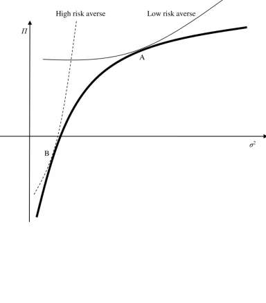
Hence, a payoff curve can be drawn as the bold line on the Π–σ2 plane in Figure 1. The thin
solid line in Figure 1 indicates the indifference curve of the bluffer that has a point of contact at
A with the payoff curve. At point A, the bluffer undertakes a bluff.
For simplicity, additional assumptions are introduced. In every period, the bluffer can
undertake one bluff because of financial constraints, and the chances of a bluff being made at any point on the curve in the Π–σ2 plane occur randomly. That is, in a given period, a bluff
succeeds with the probability p if a bluff that corresponds to point A on the curve in the Π–σ2
plane occurs. If the chances of a bluff corresponding to point A do not occur frequently and p is small, then a bubble-like phenomenon caused by a bluff will not necessarily be frequently observed.
In the case of a more risk averse bluffer, the shape of indifference curve will be something
like the thin dotted line shown in Figure 1. A bluff will not be undertaken in this case because the bluffer’s indifference curve has a point of contact at B with the payoff curve, but at point B, payoffs are negative and thus the bluff is not profitable. Nevertheless, bluffers are likely to be less risk
averse than ordinary people. Hence, the shape of the bluffer’s indifference curve will usually
resemble the thin solid line in Figure 1 where the payoff (Π) at point A is positive.
3.4.2 Initial costs
The occurrence probability of a bubble-like phenomenon caused by a bluff will be different
depending on the value of π because point A varies depending on π. Suppose that p is identical for any π. Because
2
22 2
2 p p
π
d
σ
d
as π increases, Π decreases and σ2
pp2
ππ
2 ,
π π
p p
π
d
dσ
2
2 2
, and
2
2 2 2
2 p p
π
d
σ
d
increase. Therefore, when π increases, the bold solid line shifts to the bold
dashed line in Figure 2, and point A moves to the point A′. Π for A′ is smaller than Π for A. As
π increases, Π decreases and eventually becomes negative. Hence, ifπis sufficiently large, even if the bluffer’s degree of risk averseness is very low, the bluffer will not undertake a bluff
because the expected payoffs for a bluff are negative. Conversely, ifπis sufficiently small, the bluffer will undertake a bluff even if the bluffer’s degree of risk averseness is relatively high.
3.5 The end of a bluff
As shown in Section 2, once a bluff succeeds, the economy proceeds “normally” and steadily on
the path calculated based on the manipulated expected RTP RH until households detect that a bluff has occurred. If the bluffer can successfully continue to hide their intentions, households
do not doubt that they are behaving optimally. Nevertheless if households detect the bluff, the bubble-like phenomenon will end. However, how do households detect a bluff? As Section 2 demonstrated, the economy looks to be proceeding “normally” on a path that was expected to be
optimal. In addition, most observed economic data are consistent with this expected optimal path and can be interpreted as indicating that the economy is quite normal.
There are two ways of detecting a bluff. First, authorized information suggesting the existence of the bluff may be provided by the government. Here, the supervising financial
authority plays an important role. Unlike households, the financial authority has special powers of investigation. If its supervision is sufficiently prudent and extensive, it is likely that the
authority will eventually uncover the bluff. When the financial authority perceives the existence of a bluff, it has the power to force the bluffer to stop bluffing and provide this information to
households. In this sense, prudential supervision is crucially important to help households avoid the damages inflicted on them by bluffers. The importance of the financial authority’s
supervision conversely indicates that, if households begin to doubt whether the authority’s supervision is sufficiently prudent, they may adjust the expected RTP RH largely supposing that
the current economic boom is caused by a bluff because the supervision has failed. The bluff and bubble-like phenomenon will end when households begin to doubt either the supervising authority.
A second possible way of detecting a bluff is if the bluffer pushes too far because of greed. The bluffer may have to take on a high level of risk of being detected to obtain greater
will increase as the bluffer pursues greater amounts money. A bluffer who has become
complacent or conceited because of the success of the bluff may indeed engage in such high-risk behavior. This possibility appears to be likely because bluffers are quite likely to be
greedy by nature. The bluffer does not work hard to gain profits by producing and selling better goods and services more cheaply, but by disseminating contaminated information. This behavior clearly indicates that they are intrinsically greedy.
When a bluff is detected, households will not only return the expected RTP RH to the former value, but they may go further. That is, they may generate a much higher expected RTP
RH than the original one (before the bluff) because the credibility of the financial authority has been undermined and therefore future uncertainty about the economy increases. The structural
model of RTP indicates that an increase in future uncertainty increases RTP (see the Appendix and Harashima, 2014a, b), so the expected RTP RH will be changed to a higher value than that
before the bluff. The subsequent economic stagnation will worsen as compared with the case where the expected RTP RH simply returns to the pre-bluff value.
3.6 The bluffer is not a noise trader or criminal
Although a bubble-like phenomenon generated by a bluff is not a rational bubble as defined in
bubble theory, it can be observed even if all agents behave rationally and have infinite horizons. A bubble-like phenomenon is generated not because of irrationality, but rather because of
fragility in the belief and expectation of the RTP RH as shown in Section 2. This fragility provides the opportunity for bluffers. Hence, the bluffer is not a noise trader because noise
traders are irrational and bluffers behave completely rationally. In fact, both households and bluffers behave quite rationally.
Furthermore, a bluff is not a crime in most, if not all, countries. “Pump and dump” stock sales are a crime in most countries because false news is intentionally disseminated to
gain profits. Although the bluffer contaminates information similar to a pump and dump strategy, false news is not actually disseminated. Instead, the bluffer engages in equivocal
behavior and confuses households, but the bluffer’s behavior itself is not false news. The
interpretation of the bluffer’s actions is completely up to households. Even if households wrongly interpret them, the bluffer is not responsible for their wrong interpretation. In theory, confusing households could be ruled out by law, but there are many kinds of economic activities that have the potential to confuse households to a greater or lesser extent. It would be very
difficult to enact a law that strictly defines a bluff, while also distinguishing it from other confusing activities. Bluffs therefore should not be controlled by law enforcement agencies, but
4 CONCLUDING REMARKS
Rational bubbles and economic booms led by them are not theoretically possible if agents have infinite horizons. However, assuming irrationality ad hoc does not appear to be a compelling argument. Even if people are rational and have infinite horizons, a bubble-like phenomenon can be generated if the expectation of the future economic path is hindered by some factors. In this paper, I show that bluffs are such a factor. The bluffer manipulates the household’s expected
RTP RH by acting in such a way as to lead people to believe incorrect information. A bluffer can thereby generate a bubble-like phenomenon even if people are rational and have infinite
horizons because the expected RTP RH is the discount factor that is used to determine the expected future economic path.
An example of bluff is the injection of a huge amount of money into financial markets to give loans or buy assets that would usually be regarded too risky. Bluffs are effective because
each household must generate an expected RTP RH ex ante for it to behave optimally and the expected RTP RH has to be formed based on beliefs about RTP RH. The bluffer exploits the
opportunity provided by the fragility of the expectation.
The driving force behind bluffs is greed because bluffers do not work hard to get
APPENDIX
A1 The representative household in dynamic models
A1.1 The assumption of the representative household
The concept of the representative household is a necessity in macroeconomic studies. It is used as a matter of course, but its theoretical foundation is fragile. The representative household has
been used given the assumption that all households are identical or that there exists one specific individual household, the actions of which are always average among households (I call such a
household “the average household” in this paper). The assumption that all households are identical seems to be too strict; therefore, it is usually assumed explicitly or implicitly that the
representative household is the average household. However, the average household can exist only under very strict conditions. Antonelli (1886) showed that the existence of an average
household requires that all households have homothetic and homogeneous utility functions. This type of utility function is not usually assumed in macroeconomic studies because it is very restrictive and unrealistic. If more general utility functions are assumed, however, the
assumption of the representative household as the average household is inconsistent with the assumptions underlying the utility functions.
Nevertheless, the assumption of the representative household has been widely used, probably because it has been believed that the representative household can be interpreted as an
approximation of the average household. Particularly in static models, the representative household can be seen to approximate the average household. However, in dynamic models, it
is hard to accept the representative household as an approximation of the average household because, if RTPs of households are heterogeneous, there is no steady state where all of the
optimality conditions of the heterogeneous households are satisfied (Becker, 1980). Therefore, macroeconomic studies using dynamic models are fallacious if the representative household is
assumed to approximate the average household.
A1.2 The representative household in static models
Static models are usually used to analyze comparative statics. If the average household is represented by one specific unique household for any static state, there will be no problem in
assuming the representative household as an approximation of the average household. Even though the average household is not always represented by one specific unique household in
household assumption can be used to approximate the average household.
Suppose, for simplicity, that households are heterogeneous such that they are identical except for a particular preference. Because of the heterogeneous preference, household
consumption varies. However, levels of consumption will not be distributed randomly because the distribution of consumption will correspond to the distribution of the preference. The consumption of a household that has a very different preference from the average will be very
different from the average household consumption. Conversely, it is likely that the consumption of a household that has the average preference will nearly have the average consumption. In
addition, the order of the degree of consumption will be almost unchanged for any static state because the order of the degree of the preference does not change for the given state.
If the order of consumption is unchanged for any given static state, it is likely that the household with consumption that is closest to the average consumption will also always be a
household belonging to a group of households that have very similar preferences. Hence, it is possible to argue that, approximately, one specific unique household’s consumption is always
average for any static state. Of course, it is possible to show evidence that is counter to this argument, particularly in some special situations, but it is likely that this conjecture is usually
true in normal situations, and the assumption that the representative household approximates the average household is acceptable in static models.
A1.3 The representative household in dynamic models
In dynamic models, however, the story is more complicated. In particular, heterogeneous RTPs
pose a serious problem. This problem is easily understood in a dynamic model with exogenous technology (i.e., a Ramsey growth model). Suppose that households are heterogeneous in RTP, degree of risk aversion (ε), and productivity of the labor they provide. Suppose also for
simplicity that there are many “economies” in a country, and an economy consists of a
household and a firm. The household provides labor to the firm in the particular economy, and the firm’s level of technology (A) varies depending on the productivity of labor that the household in its economy provides. Economies trade with each other: that is, the entire
economy of a country consists of many individual small economies that trade with each other.
A household maximizes its expected utility, E
u
ct
θt
dt
exp
0 , subject to
t tt f k c
k , where u
is the utility function; f
is the production function; θ isRTP; E is the expectation operator;
t t t
L Y y ,
t t t
L K k , and
t t t
L C
c ; Yt (≥ 0) is output, Kt (≥ 0)
consumption path of this Ramsey-type growth model is
θ
k y
ε
c c
t t
t
t 1
,
and at steady state,
θ
k y
t t
. (A1)
Therefore, at steady state, the heterogeneity in the degree of risk aversion (ε) is irrelevant, and the heterogeneity in productivity does not result in permanent trade imbalances among
economies because
t t
k y
in all economies is kept equal by market arbitrage. Hence,
heterogeneity in the degree of risk aversion and productivity does not matter at steady state.
Therefore, the same logic as that used for static models can be applied. Approximately, one specific unique household’s consumption is always average for any time in dynamic models,
even if the degree of risk aversion and the productivity are heterogeneous. Thus, the assumption of the representative household is also acceptable in dynamic models even if the degree of risk
aversion and the productivity are heterogeneous.
However, equation (A1) clearly indicates that heterogeneity in RTP is problematic. As
Becker (1980) shows, if RTP is heterogeneous, the household that has the lowest RTP will eventually possess all capital. With heterogeneous RTPs, there is no steady state where all
households achieve all of their optimality conditions. In addition, the household with consumption that is average at present has a very different RTP from the household with consumption that is average in the distant future. The consumption of a household that has the
average RTP will initially be almost average, but in the future the household with the lowest RTP will be the one with consumption that is almost average. That is, the consumption path of
the household that presently has average consumption is notably different from that of the household with average consumption in the future. Therefore, any individual household cannot
be almost average in any period and thus cannot even approximate the average household. As a result, even if the representative household is assumed in a dynamic model, its discounted
expected utility E
u
ct
θt
dt
exp
0 is meaningless, and analyses based on it are
If we assume that RTP is identical for all households, the above problem is solved.
However, this solution is still problematic because that assumption is not merely expedient for the sake of simplicity; rather, it is a critical requirement to allow for an assumed representative
household. Therefore, the rationale for identical RTPs should be validated; that is, it should be demonstrated that identical RTPs are actually and universally observed. RTP is, however, unquestionably not identical among households. Hence, it is difficult to accept the
representative household assumption in dynamic models based on the assumption of identical RTP.
The conclusion that the representative household assumption in dynamic models is meaningless and leads to fallacious results is very important, because a huge number of studies
have used the representative household assumption in dynamic models. To solve this severe problem, an alternative interpretation or definition of the representative household is needed.
Note that in an endogenous growth model the situation is even more complicated. Because a heterogeneous degree of risk aversion also matters, the assumption of the
representative household is more difficult to accept, so an alternative interpretation or definition is even more important when endogenous growth models are used.
A2 Sustainable heterogeneity
A2.1 The model
Suppose that two heterogeneous economies―economy 1 and economy 2—are identical except for their RTPs. Households within each economy are assumed to be identical for simplicity. The
population growth rate is zero. The economies are fully open to each other, and goods, services, and capital are freely transacted between them, but labor is immobilized in each economy.
Each economy can be interpreted as representing either a country (the international
interpretation) or a group of identical households in a country (the national interpretation).
Because the economies are fully open, they are integrated through trade and form a combined economy. The combined economy is the world economy in the international interpretation and the national economy in the national interpretation. In the following discussion, a model based
on the international interpretation is called an international model and that based on the national interpretation is called a national model. Usually, the concept of the balance of payments is used
only for the international transactions. However, because both national and international interpretations are possible, this concept and terminology are also used for the national models
in this paper.
production function in economy 1 is y1,t Aαf
k1,t and that in economy 2 is
,tα
,t A f k
y2 2 , where yi,t and ki,t are, respectively, output and capital per capita in economy i
in period t for i = 1, 2; A is technology; and α
0α1
is a constant. The population of eacheconomy is 2
L; thus, the total for both is L, which is sufficiently large. Firms operate in both
economies. The current account balance in economy 1 is τt and that in economy 2 is –τt. The
production functions are specified as
yi,t Aαki,1tα ;
thus, Yi,t Ki1,tα
ALα i1,2
. Because A is given exogenously, this model is an exogenoustechnology model (Ramsey growth model). The examination of sustainable heterogeneity based
on an endogenous growth model is shown in Appendix.
Because both economies are fully open, returns on investments in each economy are
kept equal through arbitration, such that
,t ,t ,t ,t k y k y 2 2 1 1
. (A2)
Because equation (A2) always holds through arbitration, equations k1,t k2,t , k1,t k2,t,
t t y
y1, 2, , and y1,t y2,t also hold.
The accumulated current account balance
tτsds0 mirrors capital flows between the
two economies. The economy with current account surpluses invests them in the other economy.
Because
t t t t k y k y , 2 , 2 , 1 ,
1 are returns on investments,
ds τ k y t s t t
0 , 1 ,1 and
ds τ k y t s t t
0 , 2 , 2represent income receipts or payments on the assets that an economy owns in the other economy. Hence, ds τ k y τ t s t t
t
0 , 2 , 2
t t
s t
t τ
ds
τ
k y
0 , 1, 1
is that of economy 2. Because the current account balance mirrors capital flows between the
economies, the balance is a function of capital in both economies, such that
τt κ
k1,t,k2,t
.The government (or an international supranational organization) intervenes in the
activities of economies 1 and 2 by transferring money from economy 1 to economy 2. The amount of transfer in period t is gt, and it is assumed that gt depends on capital inputs, such that
gt gk1,t ,
where g is a constant. Because k1,t k2,t and k1,t k2,t,
gt gk1,t gk2,t .
Each household in economy 1 therefore maximizes its expected utility
E
0 u1
c1,t exp
θ1t
dt
,
subject to
t ,tt
s
α
,t
α
,t
α
,t
α
t A k c α A k τ ds τ gk
k 1 1 0 1
1 1 ,
1 1
, (A3)
and each household in economy 2 maximizes its expected utility
E
0 u2
c2,t exp
θ2t
dt
,
t t t s α t α ,t α t αt A k c α A k τ ds τ gk
k 2,
0 , 2 2 1 , 2 ,
2 1
, (A4)
where ui,t and ci,t, respectively, are the utility function and per capita consumption in economy i
in period t for i = 1, 2; and E is the expectation operator. Equations (A3) and (A4) implicitly assume that each economy does not have foreign assets or debt in period t = 0.
A2.2 Sustainable heterogeneity
without government intervention
Heterogeneity is defined as being sustainable if all of the optimality conditions of all
heterogeneous households are satisfied indefinitely. First, the natures of the model when the government does not intervene (i.e., g0) are examined. The growth rate of consumption in economy 1 is
1 1 0 1 , 1 1 0 , 1 , 1 1 , 1 ,1 1 1 1 θ
k τ ds τ k A α α k ds τ k A α k A α ε c c ,t t t s α t α ,t t s α t α α t α t t . Hence,
1
1
1
0lim lim 1 1 0 1 , 1 1 0 , 1 , 1 1 , 1 , 1
k θ
τ ds τ k A α α k ds τ k A α k A α ε c c ,t t t s α t α ,t t s α t α α t α t t t t and thereby
lim
1
1
1
1
1 0 α A k α Ψ Ξ θ
α
,t
α
t ,
where t t t t t t k τ k τ Ξ , 2 , 1 lim lim
and
,t t s t ,t t s t k ds τ k ds τ Ψ 2 0 1 0 lim
lim
. t t t t t t c c y y , 1 , 1 , 1 , 1 lim
lim
0 lim
lim
1
1
t t t ,t ,t t τ τ k
k
, and Ψ is constant at steady state because k1,t and τt are constant; thus,
t t t k τ Ξ , 1 lim
is constant at steady state. For Ψ to be constant at steady state, it is necessary that
0 lim
t
1
1
1
0 lim 1 1
α A k α Ψ θ
α
,t
α
t
, (A5)
and
1
1
1
0lim 2 2
α A k α Ψ θ
α
,t
α
t
because
lim lim
1
1
1
02 2 0 1 , 2 2 0 , 2 , 2 1 , 2 , 2
k θ
τ ds τ k A α α k ds τ k A α k A α ε c c ,t t t s α t α ,t t s α t α α t α t t t t .
Because lim
1 α
Aαk1,tα
1
1 α
Ψ
θ1t
, lim
1 α
A k2
1
1 α
Ψ
θ2α
,t
α
t
,
and α ,tα α ,tα
t t t t k A k A k y k
y
2 1 . 2 , 2 . 1 ,
1 , then
t t t k y α θ θ Ψ . 1 , 1 2 1 lim 1 2 . (A6)
By equations (A5) and (A6),
11 1
1
1 lim 1
lim α Ψ θ
k y k y .t ,t t .t ,t
t
; thus, .t ,t t .t ,t t k y θ θ k y 2 2 2 1 1 1 lim 2 lim
. (A7)
If equation (A7) holds, all of the optimality conditions of both economies are indefinitely
satisfied. The state indicated by equation (A7) is called the “multilateral steady state” or
endogenous growth model in Appendix, the condition of the multilateral steady state for H
economies that are identical except for their RTPs is shown as
H θ k y H q q i.t i,t t
1lim (A8)
for any i, where i = 1, 2, … , H. Because
1
lim
1
02 1 2
2 1 . 1 , 1 2 1 θ θ α θ θ k y α θ θ Ψ t t t
by equation (A7), then by lim 0
1
0
k Ψ
ds τ ,t t s t , lim 0 0
τ dst
s t
;
that is, economy 1 possesses accumulated debts owed to economy 2 at steady state, and economy 1 has to export goods and services to economy 2 by
α
Aαktα
tτsds0 , 1
1
in every period to pay the debts. Nevertheless, because lim 0 t
t τ
and Ξ0, the debts do
not explode but stabilize at steady state. Because of the debts, the consumption of economy 1 is smaller than that of economy 2 at steady state under the condition of sustainable heterogeneity.
Note that many empirical studies conclude that RTP is negatively correlated with income (e.g., Lawrance, 1991; Samwick, 1998; Ventura, 2003). Suppose that, in addition to the
heterogeneity in RTP (θ1 < θ2), the productivity of economy 1 is higher than that of economy 2.
At steady state, the consumption of economy 1 would be larger than that of economy 2 as a
heterogeneity. Which effect prevails will depend on differences in the degrees of heterogeneity.
For example, if the difference in productivity is relatively large whereas that in RTP is relatively small, the effect of the productivity difference will prevail and the consumption of economy 1
will be larger than that of economy 2 at steady state under sustainable heterogeneity.
A3 An alternative definition of the representative household
A3.1 The definition
Section A2 indicates that, when sustainable heterogeneity is achieved, all heterogeneous
households are connected (in the sense that all households behave by considering other households’ optimality) and appear to be behaving collectively as a combined supra-household
that unites all households, as equations (A7) and (A8) indicate. The supra-household is unique and its behavior is time-consistent. Its actions always and consistently represent those of all households. Considering these natures of households under sustainable heterogeneity, I present
the following alternative definition of the representative household: “the behavior of the representative household is defined as the collective behavior of all households under
sustainable heterogeneity.”
Even if households are heterogeneous, they can be represented by a representative
household as defined above. Unlike the representative household defined as the average household, the collective representative household reaches a steady state where all households
satisfy all of their optimality conditions in dynamic models. In addition, this representative household has a RTP that is equal to the average RTP as shown in equations (A7) and (A8).2
Hence, we can assume not only a representative household but also that its RTP is the average rate of all households.
A3.2 Universality of sustainable heterogeneity
An important point, however, is that this alternatively defined representative household can be
used in dynamic models only if sustainable heterogeneity is achieved, but this condition is not necessarily always naturally satisfied. Sustainable heterogeneity is achieved only if households
with lower RTPs behave multilaterally or the government appropriately intervenes. Therefore, the representative household assumption is not necessarily naturally acceptable in dynamic models unless it is confirmed that sustainable heterogeneity is usually achieved in an economy.
Notwithstanding this flaw, the representative household assumption has been widely
2 If sustainable heterogeneity is achieved with the help of the government’s intervention, the time
used in many macroeconomic studies that use dynamic models. Furthermore, these studies have
been little criticized for using the inappropriate representative household assumption. In addition, in most economies, the dire state that Becker (1980) predicts has not been observed
even though RTPs of households are unquestionably heterogeneous. These facts conversely indicate that sustainable heterogeneity―probably with government interventions―has been usually and universally achieved across economies and time periods. In a sense, these facts are
indirect evidence that sustainable heterogeneity usually prevails in economies.
Note that because the representative household’s behavior in dynamic models is
represented by the collective behavior of all households under sustainable heterogeneity, RH’s RTP is not intrinsically known to households, but they do need to have an expected rate. Each
household intrinsically knows its own preferences, but it does not intrinsically know the collective preference of all households. Therefore, in dynamic models, it must be assumed that
all households do not ex ante know RH’s RTP, but households estimate it from information on the behaviors of other households and the government.
A4 NEED FOR AN EXPECTED RTP RH
A4.1 The behavior of household
Achieving sustainable heterogeneity affects the behavior of the individual household because sustainable heterogeneity indicates that each household must consider the other households’
optimality (as well as the behavior of the government, if necessary). This feature does not mean that households behave cooperatively with other households. Each household behaves
non-cooperatively based on its own RTP, but at the same time, it behaves considering whether
the other households’ optimality conditions are achieved or not. This consideration affects the actions a household takes in that it affects the choice of a household’s initial consumption.
Sustainable heterogeneity indicates that a household’s future path of consumption has
to be consistent with the future path of sustainable heterogeneity. Thereby, a household sets its initial consumption such that it will proceed on the path that is consistent with the path of
sustainable heterogeneity and eventually reach a steady state.
A4.2 Deviation from sustainable heterogeneity
A4.2.1 Political elements
What happens if a household deviates from sustainable heterogeneity? A deviation means that a household sets its initial consumption at a level that is not consistent with sustainable
to satisfy all of their optimality conditions is to set their initial consumption consistent with
sustainable heterogeneity. Therefore, they will not take the initiative to deviate. In contrast, the most advantaged households (i.e., those with the lowest RTP) can satisfy all of their optimality
conditions even if they set initial consumption independent of sustainable heterogeneity. The incentive for the most advantaged household to select a multilateral path will be weak because the growth rate of the most advantaged household on the multilateral path is lower than that on
the unilateral path.
When economy 1 selects the unilateral path, does economy 2 quietly accept the
unfavorable consequences shown in Becker (1980)? From an economic perspective, the optimal response of economy 2 is the one shown in Harashima (2010): economy 2 should behave as a
follower and accept the unfavorable consequences. However, if other factors—particularly political ones—are taken into account, the response of economy 2 will be different. Faced with
a situation in which all the optimality conditions cannot be satisfied, it is highly likely that economy 2 would politically protest and resist economy 1. It should be emphasized economy 2
is not responsible for its own non-optimality, which is a result of economy 1’s unilateral behavior in a heterogeneous population. Economy 2 may overlook the non-optimality if it is
temporary, but it will not if it is permanent. As shown in Harashima (2010), the non-optimality is permanent, it is quite likely that economy 2 will seriously resist economy 1 politically.
If economy 1 could achieve its optimality only on the unilateral path, economy 1 would counter the resistance of economy 2, but this is not the case. Because of this, economy
2’s demand does not necessarily appear to be unreasonable or selfish. Faced with the protest and resistance by economy 2, economy 1 may compromise or cooperate with economy 2 and select the multilateral path.
A4.2.2 Resistance
The main objective of economy 2 is to force economy 1 to select the multilateral path and to
establish sustainable heterogeneity. This objective may be achieved through cooperative measures, non-violent civil disobedience (e.g., trade restrictions), or other more violent means.
Restricting or abolishing trade between the two economies will cost economy 1 because it necessitates a restructuring of the division of labor, and the restructuring will not be
confined to a small scale. Large-scale adjustments will develop that involve all levels of divided labor, because they are all correlated with each other. For example, if an important industry had
previously existed only in one economy, owing to a division of labor, and trade between the two economies was no longer permitted, the other economy would have to establish this industry
More developed economies have more complicated and sophisticated divisions of labor, and
restructuring costs from the disruption of trade will be much higher in developed economies. In addition, more resources will need to be allocated to the generation of technology because
technology will also no longer be traded. Finally, all of the conventional benefits of trade will be lost. Trade is beneficial because of the heterogeneous endowment of resources, as the Heckscher-Ohlin theorem shows. Because goods and services are assumed to be uniform in the
models presented in this paper, the benefits of trade are implicit in the models. However, in the real word, resources such as oil and other raw materials are unevenly distributed, so a disruption
or restriction of trade will substantially damage economic activities on both national and international levels.
The damage done by trade restrictions has an upper limit, however, because the restructuring of the division of labor, additional resource allocation to innovation, and loss of
trade benefits are all finite. Therefore, in some cases, particularly if economies are not sufficiently developed and division of labor is not complex, the damage caused will be
relatively small. Hence, a disruption of trade (non-violent civil disobedience in the national models) may not be sufficiently effective as a means of resistance under some these conditions.
In some cases, harassment, sabotage, intimidation, and violence may be used, whether legal or illegal. In extreme cases, war or revolution could ensue. In such cases, economy 1 will
be substantially damaged in many ways and be unable to achieve optimality. The resistance and resulting damages will continue until sustainability is established.
In any case, the objective of economy 2’s resistance conversely implies that
establishing sustainability eliminates the risk and cost of political and social instability. The resistance of economy 2 will lower the desire of economy 1 to select the unilateral path.
A4.2.3 United economies
An important countermeasure to the fragility of sustainable heterogeneity for less advantaged
economies is the formation of a union of economies. If economies other than economy 1 are united by commonly selecting the multilateral path within them, their power to resist economy 1
will be substantially enhanced. Consider the multi-economy model shown in Harashima (2010). If the economies do not form a union, the power to resist the unilateral actions of economy 1 is
divided and limited to the power of each individual economy. However, if the economies are united, the power to resist economy 1 increases. If a sufficient number of economies unite, the
multilateral path will almost certainly be selected by economy 1.
To maintain the union, any economy in the union should have the explicit and
advantaged within the union. To demand that relatively more advantaged economies select the
multilateral path, less advantaged economies themselves must also select the multilateral path in any case. Otherwise, less advantaged economies will be divided and ruled by more advantaged
economies. For all heterogeneous people to happily coexist, all of them should behave multilaterally. At the same time, Harashima (2010) indicates that the more advantaged an economy is, the more modestly it should behave, i.e., the more it should restrain itself from
accumulating extra capitals.
In general, therefore, the most advantaged (the lowest RTP) household will be forced
to set its initial consumption consistent with sustainable heterogeneity.
A4.3 Need for an expected RTP RH
Because all households need to set their initial consumption consistent with sustainable heterogeneity to achieve it, households must calculate the path of sustainable heterogeneity
before setting their initial consumption levels. To calculate this level, each household first must know the value of RTP RH. However, although a household naturally knows the value of its
own RTP, it does not intrinsically know the value of RTP RH. To know this, a household would
have to know the values of all of the other households’ RTPs. Hence, the expected value of RTP RH must somehow be generated utilizing all other relevant available information. The necessity of an expected RTP RH is critically important because RTP plays a crucial role as the discount
factor in dynamic models.
Note that, if we assume that RTP is identical for all households, an expected RTP RH
is no longer needed because any household’s own RTP is equal to the RTP RH. This solution is still problematic, however, because the assumption is not merely expedient for the sake of simplicity; rather, it is a critical requirement to eliminate the need for an expected RTP RH.
Therefore, any rationale for assuming identical RTPs should be validated; that is, it should be
demonstrated that identical RTPs do exist and are universally observed. However, RTP is unquestionably not identical among households. Therefore, households must use expected values of RTP RH.
A5 THE RTP MODEL
A5.1 Need to know the structural model
If RTP RH is a constant parameter, as has been long and widely assumed, the need for an expected RTP RH would not be a serious problem. The historical mean of an unchanging RTP
indicators even if the structural model remained unknown. The RTP RH could be specified as
the RTP that is most consistent with long-term trends of the indicators.
Although RTP has been treated as a constant parameter in many studies, this feature
has not been demonstrated either empirically or theoretically. Rather, the assumption is merely expedient for the sake of simplicity. There is another practical reason for this treatment: models with a permanently constant RTP exhibit excellent tractability (see Samuelson, 1937). However,
some have argued that it is natural to view RTP as temporally variable, and the concept of a temporally varying RTP has a long history (e.g., Böhm-Bawerk, 1889; Fisher, 1930). More
recently, Lawrance (1991) and Becker and Mulligan (1997) showed that people do not inherit permanently constant RTPs by nature and that economic and social factors affect the formation
of RTPs. Their arguments indicate that many incidents can affect and change RTP. Models of
endogenous RTP have been presented, the most familiar of which is Uzawa’s (1968) model.
If the RTP RH is temporally variable, its future stream must be expected by households, and a rational expectation is a model-consistent expectation. To generate rational
expectations of RTP RH, therefore, the structural model of the RTP RH (i.e., equations that fundamentally describe how it is endogenously formed) needs to be known.
A5.2 Endogenous RTP models
A5
.2.1 Uzawa’s (1968) model
The most well-known endogenous RTP