Selection of an estimation window in the presence of data revisions and recent structural breaks

Munich Personal RePEc Archive

Selection of an estimation window in the

presence of data revisions and recent

structural breaks

Hännikäinen, Jari

University of Tampere

18 September 2015

Online at

https://mpra.ub.uni-muenchen.de/66826/

T A M P E R E E C O N O M I C W O R K I N G P A P E R S

N E T S E R I E S

SELECTION OF AN ESTIMATION WINDOW IN

THE PRESENCE OF DATA REVISIONS AND

RECENT STRUCTURAL BREAKS

Jari Hännikäinen

Working Paper 92

September 2015

SCHOOL OF MANAGEMENT

FI-33014 UNIVERSITY OF TAMPERE, FINLAND

Selection of an estimation window in the presence of

data revisions and recent structural breaks

∗

Jari H¨

annik¨

ainen

September 2015

Abstract

In this paper, we analyze the forecasting performance of a set of widely used

window selection methods in the presence of data revisions and recent structural

breaks. Our Monte Carlo and empirical results for U.S. real GDP and inflation

show that the expanding window estimator often yields the most accurate

fore-casts after a recent break. It performs well regardless of whether the revisions

are news or noise, or whether we forecast first-release or final values. We find

that the differences in the forecasting accuracy are large in practice, especially

when we forecast inflation after the break of the early 1980s.

Keywords: Recent structural break, choice of estimation window,

forecast-ing, real-time data

JEL codes: C22, C53, C82

∗_{I would like to thank Henri Nyberg, Juuso Vataja, Jari Vainiom¨aki, Helin¨a Laakkonen, Markku}

1.

Introduction

Macroeconomic time series are often serially correlated. This implies that their own past

values are themselves useful predictors. Therefore, it is not surprising that autoregressive

(AR) models are used extensively in economic forecasting. The previous literature has found

that it is difficult to outperform AR models in practice. For example, Rossi (2013) and Stock

and Watson (2003) find that only a few macroeconomic predictors systematically improve

upon the AR benchmark when forecasting inflation and output growth.

However, the parameters of AR models fitted to many macroeconomic time series are

unstable over time (see, e.g., Stock and Watson, 1996). This observed parameter instability

can arise as a result of several reasons. For instance, changes in tastes, technology, legislation,

institutional arrangements, or government policy can cause changes in the dynamics of the

economy. Structural breaks are crucial because they often have a major impact on forecasting

performance: a forecasting model that performed well before the break might perform

ex-tremely poorly after the break (see, e.g., Clements and Hendry, 1998; Rossi, 2013). Because

tastes, technology, legislation, institutional arrangements, and government policy are likely

to change in the future, structural breaks are also likely to happen in the future. Therefore,

information about the forecasting performance of AR models when these models undergo

structural breaks is needed. Given the empirical success of AR models and their widespread

use in practice, we believe that this is an important area to investigate.

A key question in the presence of structural instability is how many observations to use to

estimate the parameters of a model so that, when used to generate a forecast, a loss function

such as the root mean squared forecast error (RMSFE) will be minimized. This issue has

been analyzed by Eklund et al. (2013), Giraitis et al. (2013), Pesaran and Pick (2011),

Pesaran and Timmermann (2005, 2007), and Pesaranet al. (2013). This literature typically

assumes that the break has occurred in the distant past. In such a case, the standard solution

to the window selection problem is to test for breaks and use only observations after the most

recent break. The estimates of the timing of the break(s) can be obtained, for example, using

methods developed by Altissimo and Corradi (2003), Andrews (1993), Andrewset al. (1996),

and Bai and Perron (1998, 2003). In the presence of recent breaks, this so called post-break

window strategy is not feasible. As noted by Eklund et al. (2013), structural break tests

are not designed for detecting recent breaks. Instead, the breaks are observed with a long

lag. Even if real-time detection were possible, the post-break window strategy would not be

useful. The parameters of the forecasting model are estimated with adequate accuracy only if

the number of observations is at least two to three times the number of parameters (see, e.g.,

the discussion in Pesaran and Timmermann, 2005). Hence, the post-break window strategy

is applicable only when the (last) break has occurred sufficiently long ago.

Forecasting after a recent break has received very little attention in the literature.

How-ever, in practice, forecast errors are often very large after structural breaks (Clements and

Hendry, 2006). This suggests that improving forecast accuracy after a recent break is a

central issue in economic forecasting.

Another issue that has often been overlooked in the literature is the real-time nature of

the data used in many applications. For example, GDP and inflation series are published

with a lag and are subject to revisions. These revisions are usually quite large and hence

forecasts based on final revised data may differ considerably from those based on real-time

data. Practical forecasting is inherently a real-time exercise, and therefore ingnoring the

real-time nature of the data leads to a wide discrepancy between theory and practice.

We introduce two innovations on the existing literature. First, we focus on forecasting in

the presence of recent breaks. To this end, several break processes are considered, including

changes in the intercept, autoregressive parameter, and error variance. Second, we take into

account that most macroeconomic time series are subject to data revisions. We follow the

standard practice in the literature and allow revisions to be characterized either as news or

noise, in the sense of Mankiw and Shapiro (1986). To the best of our knowledge, there are no

other papers analyzing the window selection problem when the data are subject to revision.

The end of the Great Moderation and the Financial Crisis of 2008 provide an excellent

motivation for our exercise. It is well-known that the volatility of many U.S. macroeconomic

series has declined since the mid-1980s (see, e.g., McConnell and Perez-Quiros, 2000). Recent

the Financial Crisis. Furthermore, monetary policy has changed fundamentally since the

beginning of the crisis. The nominal short-term interest rate has been stuck at the zero lower

bound and the Federal Reserve has used unconventional monetary policy, both of which

should change the dynamics of key macro variables. So, forecasting these days, one would

certainly run into the aforementioned too-few-data-after-the-break problem and the results

of this paper will be relevant.

We consider a set of widely used methods for forecasting in the presence of structural

instability. These methods include rolling windows, exponentially weighted moving average

models, and the average window method advocated by Pesaran and Pick (2011) and Pesaran

and Timmermann (2007). The potential gains in forecasting performance from using these

methods compared to the expanding window method are demonstrated through Monte Carlo

simulations and empirical examples.

The main finding from this study is that, at least for macroeconomic time series such as

U.S. real GDP and inflation (defined as the growth rate of the GDP deflator), the expanding

window estimator tends to produce more accurate forecasts than the alternative window

se-lection methods considered here. Our simulation results indicate that the expanding window

method performs particularly well when the parameters remain constant over time or when

the innovation variance changes. Our empirical results suggest that the expanding window

estimator is overwhelmingly the best estimation strategy when we forecast inflation after the

break in the early 1980s. In this case, the alternative methods produce 7.5–52.9 percent

larger forecast errors than the expanding window estimator. The expanding window method

also performs well when we make real-time GDP growth forecasts for the period 2008:Q4–

2011:Q1. However, we find that, in this case, the differences in relative performances are

more modest.

The remainder of the paper is organized as follows. Section 2 introduces the notation

and the statistical framework. Section 3 provides a brief overview of the window selection

methods. Section 4 presents the Monte Carlo simulation results and Section 5 presents the

empirical results. Section 6 concludes. The appendices at the end of the paper provide the

technical details.

2.

Statistical framework

An important feature of real-time data is that the data for a period are not released until

some time has passed after the end of that period. Therefore, for instance, a forecaster

at period T+1 has access to the vintage T+1 values of real GDP and inflation up to time

periodT. Furthermore, the data are revised over time, so the first-released values and the final

values may differ considerably. Although the real-time nature of macroeconomic time series

clearly matters for forecasting, data revisions are rarely incorporated into the theoretical

models. One exception is the statistical framework suggested by Jacobs and van Norden

(2011) and further developed by Clements and Galv˜ao (2013). This framework for modeling

data revisions, which we will closely follow, relates a data vintage estimate to the true value

plus an error or errors. In particular, the period t+s vintage estimate of the value of y in

periodt, denoted byyt_t+s1 , wheres = 1,...,l 2 , can be expressed as a sum of the true value

˜

yt, a news componentvtt+s, and a noise componentεtt+s, so thatytt+s = ˜yt+vtt+s+εtt+s.

This framework follows the standard practice in the literature and assumes that revisions

either add news or reduce noise. Data revisions are said to be news if revisions are

uncorre-lated with the previously published vintages, cov(yt_t+k, v_tt+s) = 0 ∀k≤s. This implies that

the initially released data are optimal forecasts of the later data. On the other hand, data

revisions reduce noise if each vintage release is equal to the true value plus a noise, so that

noise revisions are uncorrelated with the truth, cov(˜yt, εtt+s) = 0. For further discussion of

the properties of news and noise revisions, see Croushore (2011) and Jacobs and van Norden

(2011). The distinction between news and noise revisions is important in practice because

revisions to different macroeconomic time series have different characteristics. For example,

Clements and Galv˜ao (2013) find that, at least since the mid-1980s, data revisions to output

growth appear to be mainly news whereas those to inflation are mainly noise.

Following Clements and Galv˜ao (2013) and Jacobs and van Norden (2011), we stack

1

Throughout this paper, superscripts refer to vintages and subscripts to time periods. This notation has become standard in the literature.

2

For simplicity, we assume that we observe l different estimates of yt before the true value, ˜yt, is

the l different vintage estimates of yt, vt and εt into vectors yt = (ytt+1, ..., ytt+l)

′

, vt =

(vt_t+1, ..., v_tt+l)′ and εt= (εtt+1, ..., εtt+l)

′

, respectively. Now we can express each vintage of yt

as follows

yt=iy˜t+vt+εt, (1)

whereiis anl×1 vector of ones. For the true values we consider the following AR(1) process

subject to a single structural break at timeT1

˜

yt=

          

ρ1+

l

X

i=1

µv1i+β1y˜t−1+σ1η1t+

l

X

i=1

σv1iη2t,i, fort < T1,

ρ2+

l

X

i=1

µv2i+β2y˜t−1+σ2η1t+

l

X

i=1

σv2iη2t,i, fort≥T1,

(2)

whereη1t and η2t,i (i = 1,. . . ,l) areN IID (0,1) disturbances.3

The news and noise processes of each vintage are specified by

v1t=

        

v₁t+1_t

v₁t+2_t

.. .

v₁t+_tl

         =−              l X i=1

µv1i

l

X

i=2

µv1i

.. .

µv1l

             −              l X i=1

σv1iη2t,i

l

X

i=2

σv1iη2t,i

.. .

σv1lη2t,l

            

,ε1t=

        

εt₁+1_t

εt₁+2_t

.. .

εt₁+_tl

         =−         

µε11

µε12

.. .

µε1l

         +         

σε11η3t,1

σε12η3t,2

.. .

σε1lη3t,l

         (3)

fort < T1 and

3

We focus on the shortest possible lag length, because we want to minimize the number of possible breaks in the autoregressive structure. Furthermore, it is easier to calibrate the parameters (see the discussion below) when the lag order is one. Eklund et al. (2013) and Pesaran and Timmermann (2005) also consider an AR(1) specification in the presence of breaks.

v2t=         

v₂t+1_t

v₂t+2_t

.. .

v₂t+_tl

         =−              l X i=1

µv2i

l

X

i=2

µv2i

.. .

µv2l

             −              l X i=1

σv2iη2t,i

l

X

i=2

σv2iη2t,i

.. .

σv2lη2t,l

            

,ε2t=

        

εt₂+1_t

εt₂+2_t

.. .

εt₂+_tl

         =−         

µε21

µε22

.. .

µε2l

         +         

σε21η3t,1

σε22η3t,2

.. .

σε2lη3t,l

         (4)

fort≥T1.

The shocks are assumed to be mutually independent, i.e., if η_t = hη1t,η

′

2t,η

′

3t

i′

, then

E(η_t) =0andE(η_tη_t′) =I. We assume that ˜ytis a stationary process, so that|βj|<1 (forj

= 1,2). Because ˜ytis a stationary process and both the news and noise terms are stationary,

(1) implies thaty_t is also a stationary process. Note that the means of the news and noise

terms, denoted byµvji andµεji (forj = 1,2 andi = 1,...,l), are allowed to be non-zero. This

is an important feature because in practice revisions to macroeconomic data have non-zero

means (see, e.g., Aruoba, 2008; Clements and Galv˜ao, 2013; Croushore, 2011).

As discussed earlier, this framework is similar to that adopted in Clements and Galv˜ao

(2013) and Jacobs and van Norden (2011). The main point of departure from their framework

is that we allow the process of the true values to be subject to a recent structural break. Our

setup is quite general and allows for changes in intercept, slope, and error variance

immedi-ately after the break. Another novelty of our framework is that the means and variances of

the news and noise revisions are also allowed to change.

3.

Forecasting methods

In the presence of data revisions and structural breaks, a forecaster faces two key questions.

First, a forecaster has to decide how to take into account the real-time nature of the data

when estimating the parameters of the forecasting model. The most commonly used approach,

(T+1) vintage

y_tT+1 =α0+α1ytT−+11 +et,EOS, fort= 2, ..., T. (5)

The forecast ofyT+1 is conditioned on the latest available vintage value of the forecast origin

data, so that ˆyT+1,EOS = ˆα0+ ˆα1yTT+1. Although popular in practice, the EOS approach

has a fundamental shortcoming: a large part of the data used in model estimation has been

revised many times (early in the sample), while the forecast is conditioned on first-release

data (the latest observation).

An alternative estimation strategy is the real-time vintage approach (RTV) suggested

by Koenig et al. (2003). The central idea in the RTV approach is that the data used in

estimation and the data on which the forecast is conditioned should be of a similar maturity.

Therefore, the forecasting model is estimated on first-release data

yt_t+1=β0+β1ytt−1+et,RT V, fort= 2, ..., T, (6)

and the corresponding forecast is ˆyT+1,RT V = ˆβ0+ ˆβ1yTT+1. Note that the two forecasts are

conditioned on exactly the same data. The only difference between the two approaches is the

data used in the estimation.

The results in Clements and Galv˜ao (2013) and Koenig et al. (2003) indicate that the

RTV approach produces more accurate forecasts than the EOS approach. However, it is not

known whether this result holds in the presence of structural instability. Thus, our plan is

to shed light on the relative accuracy of these two methods in the presence of recent breaks.

The second question a forecaster faces is how much data to use to estimate the parameters

of the forecasting model. One solution to this window selection problem is to test for breaks

and use only observations over a post-break window. If the structural break has occurred

recently, this post-break window strategy is infeasible for two reasons. First, it is difficult

or even impossible to estimate accurately the timing of a recent break. Second, even if an

accurate detection of a recent break were possible, the post-break window strategy is infeasible

because a sufficient number of post-break observations, say at least two to three times the

number of parameters, is required for accurate estimation. Once the real-time nature of the

data is taken into account, the problems associated with the post-break window strategy

get compounded since the break may not be as apparent in real-time. Moreover, post-break

observations are less ’mature’, which will cause problems with accuracy.

An alternative solution is to use robust estimation strategies. An estimation strategy is

said to be robust if no information about the structural break is needed for its implementation.

Therefore, robust methods are also valid in the presence of recent breaks. In this paper, we

focus exclusively on robust methods. We compare the forecasting performance of a set of

widely used estimation strategies when the underlying time series process has undergone a

recent structural break. Common to all of these strategies is that the estimation window

should exceed a minimum length, denoted byω.

The first strategy is the expanding window estimator

ˆ

β_T,EXP =

T

X

t=1

xt−1x

′

t−1

!−1 _T

X

t=1

x′_t−1yt,

where xt = (1, yt)

′

. The expanding window estimator uses the whole data sample

avail-able at the forecast origin. The expanding window forecast for periodT+1 is computed by

ˆ

yT+1,EXP = ˆβ

′

T,EXPxT.

The second strategy is the rolling window estimator

ˆ

β_T,ROLL(m) =

T

X

t=T−m+1

xt−1x

′

t−1

!−1 _T

X

t=T−m+1

x′_t−1yt,

where m ∈ ω, ..., T is the length of the rolling window. The parameters are estimated

us-ing the m most recent observations. The resulting forecast for period T+1 is computed by

ˆ

yT+1,ROLL(m) = ˆβT,ROLL(m)

′

xT. Giacomini and White (2006) argue that when the

fore-casting model is misspecified (due to inadequately modeled dynamics, inadequately modeled

heterogeneity, incorrect functional form, or any combination of these), the rolling window

estimator often provides more reliable forecasts than the expanding window estimator.

This method, unlike rolling regressions, gives a positive weight to each observation. The

cen-tral idea is that if the relation of interest has changed over time, the most recent observations

are more informative than the earlier ones. Thus, the most recent observations receive the

highest weight in the estimation:

ˆ

β_{T,EW M A}= λ

T

X

t=1

(1−λ)T−t_x

t−1x

′

t−1

!−1

λ

T

X

t=1

(1−λ)T−t_x′

t−1yt,

where 0 < λ < 1 is the down-weighting parameter. The forecast for period T+1 is

com-puted by ˆyT+1,EW M A = ˆβ

′

T,EW M AxT. Pesaran and Pick (2011) find that the choice of the

down-weighting parameter greatly affects the forecasting performance of the EWMA method.

A final alternative is the average window (AveW) method suggested by Pesaran and

Timmermann (2007). This method builds on the common finding that forecast combinations

often reduce forecast errors (see, e.g., Timmermann, 2006). Therefore, rather than selecting

a single estimation window, the AveW method combines forecasts from models estimated on

different observation windows. The AveW method gives an equal weight to each forecast,

ˆ

yT+1,AveW = (T−ω+ 1)−1 T

X

m=ω

ˆ

yT+1,ROLL(m),

where ˆyT+1,ROLL(m) denotes the forecast generated by a rolling window of size m.

4.

Monte Carlo simulations

In this section, we evaluate the forecasting performance of alternative window selection

meth-ods in a set of Monte Carlo experiments. These experiments are based on the statistical

framework introduced in Section 2. Our interest in this paper lies in the point forecasts

shortly after a structural break. Therefore, we assume that a single break has occurred at

timeT1 =T. One-step ahead forecasts are made recursively for the next ten periods, i.e., for

the periodsT+1,...,T+10. We assume that no breaks occur during the forecasting period.

To ensure that our simulation results are empirically relevant, we calibrate the

ters on actual U.S. output and inflation data. We start by considering the case where the

parameters remain stable over time (experiment 1 in Table 1). In this case the mean of

the true process lies between 2.0 and 2.5, which corresponds roughly to the average annual

inflation and real GDP growth since the mid-1980s. The parameters of this model are used

as benchmarks in the rest of the experiments. We consider both moderate (0.25) and large

(0.5) changes in the autoregressive parameter in either direction (experiments 2–5). We also

consider changes in the error variance. We allow σ to increase from 1.5 to 4.5 (experiment

6) and decrease from 1.5 to 0.5 (experiment 7). Finally, we study the effects of breaks in the

constant term (experiments 8–9).

We assume that the revisions are either pure news (σvi ̸= 0, σεi = 0 fori = 1, ...,l) or

pure noise (σvi = 0, σεi ̸= 0 fori= 1, ...,l). This allows us to analyze whether the properties

of the revision process matters for the window selection problem. We setl= 14, so that we

observe 14 different estimates ofytbefore the true value, ˜yt, is observed. Following Clements

and Galv˜ao (2013), we assume that the first and the fifth revisions are non-zero mean. The

means of these revisions are set to four and two percent of the mean of the first-release data,

yt_t+1, both before and after the break. Similarly, the standard deviation of the first revision is

set to 40 percent of the standard deviation of the first-release data. The standard deviations

of revisions 2–13 and 14 are set to 20 and 10 percent of the standard deviation of the

first-release data, respectively. For convenience, the parameter values used in the Monte Carlo

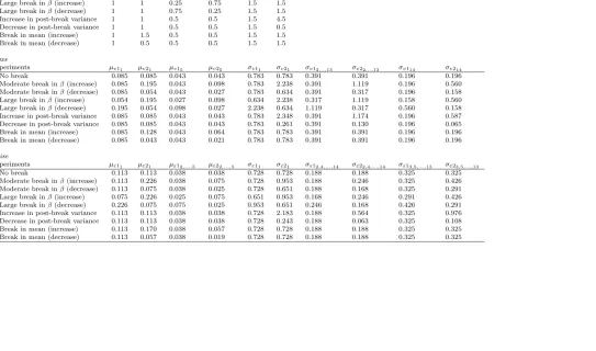
experiments are reported in Table 1.4

We examine the ability of various window selection methods to forecast both the

first-release values (yt_t+1+2) and the final values (yt_t+1+16). Because we assume that revisions have

non-zero mean, the final values differ systematically from the first-release values. As a

conse-quence, the forecasting models in (5) and (6) produce unbiased forecasts for the first-release

values, but biased forecasts for the final values. In order to produce unbiased forecasts for the

final values, we use the bias correction method suggested by Clements and Galv˜ao (2013). The

4

Table 1: Simulation setup

True process

Experiments ρ1 ρ2 β1 β2 σ1 σ2

1: No break 1 1 0.5 0.5 1.5 1.5

2: Moderate break inβ(increase) 1 1 0.5 0.75 1.5 1.5

3: Moderate break inβ(decrease) 1 1 0.5 0.25 1.5 1.5

4: Large break inβ(increase) 1 1 0.25 0.75 1.5 1.5

5: Large break inβ(decrease) 1 1 0.75 0.25 1.5 1.5

6: Increase in post-break variance 1 1 0.5 0.5 1.5 4.5

7: Decrease in post-break variance 1 1 0.5 0.5 1.5 0.5

8: Break in mean (increase) 1 1.5 0.5 0.5 1.5 1.5

9: Break in mean (decrease) 1 0.5 0.5 0.5 1.5 1.5

News

Experiments µv11 µv21 µv15 µv25 σv11 σv21 σv12,..,13 σv22,..,13 σv114 σv214

1: No break 0.085 0.085 0.043 0.043 0.783 0.783 0.391 0.391 0.196 0.196

2: Moderate break inβ(increase) 0.085 0.195 0.043 0.098 0.783 2.238 0.391 1.119 0.196 0.560

3: Moderate break inβ(decrease) 0.085 0.054 0.043 0.027 0.783 0.634 0.391 0.317 0.196 0.158

4: Large break inβ(increase) 0.054 0.195 0.027 0.098 0.634 2.238 0.317 1.119 0.158 0.560

5: Large break inβ(decrease) 0.195 0.054 0.098 0.027 2.238 0.634 1.119 0.317 0.560 0.158

6: Increase in post-break variance 0.085 0.085 0.043 0.043 0.783 2.348 0.391 1.174 0.196 0.587

7: Decrease in post-break variance 0.085 0.085 0.043 0.043 0.783 0.261 0.391 0.130 0.196 0.065

8: Break in mean (increase) 0.085 0.128 0.043 0.064 0.783 0.783 0.391 0.391 0.196 0.196

9: Break in mean (decrease) 0.085 0.043 0.043 0.021 0.783 0.783 0.391 0.391 0.196 0.196

Noise

Experiments µε11 µε21 µε12,...,5 µε22,...,5 σε11 σε21 σε12,4,...,14 σε22,4,...,14 σε13,5,...,13 σε23,5,...,13

1: No break 0.113 0.113 0.038 0.038 0.728 0.728 0.188 0.188 0.325 0.325

2: Moderate break inβ(increase) 0.113 0.226 0.038 0.075 0.728 0.953 0.188 0.246 0.325 0.426

3: Moderate break inβ(decrease) 0.113 0.075 0.038 0.025 0.728 0.651 0.188 0.168 0.325 0.291

4: Large break inβ(increase) 0.075 0.226 0.025 0.075 0.651 0.953 0.168 0.246 0.291 0.426

5: Large break inβ(decrease) 0.226 0.075 0.075 0.025 0.953 0.651 0.246 0.168 0.426 0.291

6: Increase in post-break variance 0.113 0.113 0.038 0.038 0.728 2.183 0.188 0.564 0.325 0.976

7: Decrease in post-break variance 0.113 0.113 0.038 0.038 0.728 0.243 0.188 0.063 0.325 0.108

8: Break in mean (increase) 0.113 0.170 0.038 0.057 0.728 0.728 0.188 0.188 0.325 0.325

9: Break in mean (decrease) 0.113 0.057 0.038 0.019 0.728 0.728 0.188 0.188 0.325 0.325

1

bias correction is the sample estimate of the difference between the final value and the

first-release value calculated using data up to the forecast origin. To be more specific, the forecast

for the final value is computed using the formula ˆy_tt+16₊₁ = ˆyt_t+1+2+ (t−14)−1

t−14

X

i=1

(y_ii+15−yi_i+1).

An alternative approach, of course, would be to use the fully revised data as the left hand side

variable in (5) and (6). As discussed in Clements and Galv˜ao (2013), these two approaches

are asymptotically equivalent. However, the bias correction method yields more accurate

forecasts in small samples.

We focus on a set of widely used robust estimation strategies, including the rolling

win-dow, the exponentially weighted moving average (EWMA), and the average window (AveW)

method. We analyze the forecasting performance of a short rolling window using the most

recent 20 observations and a long rolling window using the most recent 40 observations.

These rolling windows correspond to five and 10 years of quarterly data, respectively. The

down-weighting parameter, λ, in the EWMA method is set to 0.05 (henceforth EWMAS).

In addition, we follow Eklund et al. (2013) and consider a method that combines different

down-weighting parameters. More specifically, we calculate an equally weighted forecast

us-ing down-weightus-ing parameters of 0.1, 0.2 and 0.3 (henceforth EWMAA). We assume that

the minimum estimation window length,ω, in the AveW method is 10 observations.

The expanding window estimator is the most efficient estimation method when the

un-derlying time series process is stable over time. Therefore, it is used as a benchmark in our

Monte Carlo simulations. For each robust estimation strategy we compute RMSFE values

relative to those produced by the expanding window benchmark. Values below (above) unity

indicate that the candidate method produces more (less) accurate forecasts than the

bench-mark. Relative RMSFE values are computed with sample sizesT = 50, 100, and 150. The

results are based on 10,000 replications and are shown in Tables 2–5.

First, we compare the forecasting performance of alternative window selection methods

when the revisions are pure news. The results, presented in Tables 2 and 3, reveal that

the forecasting methods that generate the lowest RMSFE values in most of the experiments

are the expanding window benchmark and the EWMAS method. Indeed, the expanding

vari-able/experiment/vintage approach/sample size combinations considered here. It performs

particularly well when the parameters remain stable over time (experiment 1) or when the

variance of the time series changes (experiments 6 and 7). There is a simple explanation for

these findings. When the parameters remain fixed over time, it is optimal to use as many

observations as possible in the estimation. Similarly, when a break only affects the volatility

of the series, the variance of the parameter estimation error can be reduced by using a longer

estimation window. The expanding window estimator performs poorly only when the

autore-gressive parameter is subject to large changes (experiments 4 and 5). Such breaks imply huge

changes in the mean of the process, and are thus unlikely to occur in practice. Therefore, the

weak performance of the expanding window estimator in the presence of large slope shifts

should not be overemphasized. Interestingly, we find that it is more difficult to outperform

the benchmark when the RTV approach is used. Similarly, the expanding window method

performs better when the first-release values are the ones to be forecast.

Another prominent window selection method is the EWMAS approach. This approach

performs well when the autoregressive parameter increases substantially after the break

(ex-periment 4). In this case, the improvements over the expanding window benchmark are quite

large, ranging from 0.6 to 8 percent. The EWMAS method also does particularly well in

experiment 5 when we forecast first-release values, and in experiment 9 when we forecast the

final values. Note that the EWMAS method improves upon the benchmark more often when

the EOS approach is used.

In the few cases where the expanding window or EWMAS approach do not dominate,

the EWMAA and AveW methods generate the best forecasts. The AveW method produces

forecasts that are very close to those produced by the expanding window estimator. Therefore

both the gains and losses in relative accuracy are more modest than with the other methods.

The EWMAA method, on the other hand, performs well when the slope parameter decreases

substantially after the break (experiment 5) and we forecast the final values, but extremely

poorly in the vast majority of the experiments. The rolling windows fare no better: they

rarely improve upon the benchmark and never produce the most accurate forecasts.

Our results indicate that the choice between the EOS and RTV approaches is not

Table 2: Relative RMSFE values when revisions are news

First-release

EOS RTV

Exp. RMSFE m = 20 m = 40 EWMAS EWMAA AveW T = 50 RMSFE m = 20 m = 40 EWMAS EWMAA AveW

1 1.743 1.042 1.007 1.007 1.078 1.011 1.732 1.036 1.006 1.010 1.096 1.011

2 3.906 1.016 1.001 0.999 1.059 1.002 3.925 1.030 1.004 1.014 1.126 1.010

3 1.673 1.029 1.005 0.999 1.054 1.001 1.646 1.023 1.003 1.003 1.071 1.001

4 4.159 0.984 0.990 0.971 1.010 0.980 4.160 1.004 0.995 0.992 1.087 0.992

5 2.208 1.061 1.014 0.954 0.954 0.998 2.114 1.043 1.008 0.968 0.982 0.997

6 5.213 1.046 1.009 1.034 1.174 1.022 5.248 1.053 1.010 1.044 1.213 1.027

7 0.654 1.171 1.038 0.997 1.030 1.035 0.621 1.137 1.028 1.007 1.063 1.033

8 1.789 1.033 1.006 0.998 1.056 1.005 1.794 1.025 1.004 1.000 1.070 1.004

9 1.822 1.027 1.005 0.993 1.044 1.002 1.794 1.025 1.004 0.999 1.068 1.004

T = 100

1 1.714 1.056 1.020 1.015 1.093 1.008 1.707 1.047 1.016 1.017 1.110 1.007

2 3.917 1.011 0.996 0.991 1.051 0.992 3.920 1.028 1.003 1.008 1.121 0.997

3 1.665 1.040 1.016 1.006 1.061 1.001 1.642 1.030 1.011 1.007 1.075 1.000

4 4.302 0.955 0.962 0.941 0.980 0.962 4.275 0.980 0.972 0.966 1.062 0.970

5 2.116 1.111 1.057 0.982 0.993 1.009 2.053 1.079 1.037 0.987 1.011 1.005

6 5.149 1.057 1.021 1.041 1.187 1.015 5.166 1.072 1.027 1.057 1.243 1.020

7 0.612 1.240 1.109 1.043 1.098 1.034 0.592 1.185 1.080 1.040 1.112 1.028

8 1.782 1.041 1.015 1.004 1.066 1.002 1.793 1.032 1.010 1.003 1.077 1.001

9 1.809 1.037 1.013 0.999 1.055 1.001 1.784 1.034 1.011 1.004 1.079 1.002

T = 150

1 1.711 1.061 1.025 1.020 1.099 1.006 1.707 1.052 1.021 1.020 1.113 1.005

2 3.944 1.008 0.993 0.988 1.050 0.988 3.939 1.026 1.000 1.007 1.120 0.992

3 1.661 1.042 1.018 1.008 1.066 1.000 1.641 1.031 1.012 1.009 1.078 0.999

4 4.414 0.933 0.940 0.920 0.956 0.952 4.383 0.959 0.951 0.945 1.042 0.957

5 2.085 1.122 1.071 0.994 1.004 1.009 2.030 1.085 1.048 0.995 1.019 1.005

6 5.128 1.061 1.024 1.044 1.188 1.011 5.138 1.076 1.032 1.061 1.242 1.015

7 0.598 1.268 1.136 1.067 1.122 1.030 0.583 1.197 1.095 1.053 1.127 1.021

8 1.766 1.046 1.019 1.008 1.072 1.002 1.780 1.036 1.013 1.006 1.082 1.001

9 1.811 1.040 1.017 1.001 1.056 1.001 1.788 1.035 1.014 1.005 1.079 1.001

Notes: The experiments are as defined in Table 1. Method m = 20 denotes rolling window of size 20, whereas m = 40 denotes rolling window of size 40. EWMAS denotes EWMA method withλ= 0.05 and EWMAA denotes EWMA method withλ= 0.1, 0.2 and 0.3. AveW denotes the average window method. The sample size is T. The break occurs at periodT1=T. One-step ahead forecasts are generated recursively for periodsT+1,...,T+10. The first column in each panel shows the RMSFE

for the expanding window estimator. In subsequent columns, RMSFE values are computed relative to those produced by the expanding window estimator.

1

Table 3: Relative RMSFE values when revisions are news

Final value

EOS RTV

Exp. RMSFE m = 20 m = 40 EWMAS EWMAA AveW T = 50 RMSFE m = 20 m = 40 EWMAS EWMAA AveW

1 2.383 1.018 1.003 1.000 1.035 1.003 2.366 1.017 1.003 1.004 1.049 1.005

2 5.991 1.006 1.000 0.998 1.024 1.000 6.001 1.012 1.001 1.005 1.054 1.004

3 2.146 1.012 1.002 0.995 1.023 0.997 2.114 1.010 1.001 1.000 1.038 0.999

4 6.155 0.990 0.995 0.984 0.999 0.989 6.151 0.999 0.997 0.994 1.035 0.995

5 2.895 1.004 1.002 0.945 0.909 0.979 2.777 1.000 1.000 0.958 0.937 0.983

6 7.044 1.025 1.005 1.018 1.099 1.012 7.066 1.029 1.006 1.025 1.122 1.015

7 0.932 1.059 1.013 0.978 0.967 0.999 0.881 1.057 1.012 0.993 1.007 1.008

8 2.428 1.012 1.002 0.994 1.021 0.999 2.424 1.011 1.002 0.997 1.032 1.000

9 2.460 1.010 1.001 0.992 1.015 0.998 2.428 1.010 1.001 0.997 1.031 1.000

T = 100

1 2.345 1.027 1.010 1.006 1.048 1.003 2.335 1.024 1.009 1.008 1.059 1.003

2 6.008 1.002 0.997 0.994 1.018 0.996 6.008 1.010 1.000 1.001 1.049 0.998

3 2.129 1.021 1.009 1.001 1.032 0.999 2.103 1.017 1.006 1.003 1.043 0.999

4 6.277 0.977 0.981 0.971 0.986 0.981 6.256 0.989 0.986 0.983 1.026 0.985

5 2.688 1.051 1.030 0.970 0.952 0.999 2.613 1.035 1.019 0.976 0.970 0.998

6 7.012 1.031 1.011 1.022 1.105 1.008 7.023 1.040 1.015 1.031 1.138 1.011

7 0.852 1.111 1.050 1.008 1.023 1.010 0.823 1.090 1.039 1.014 1.044 1.011

8 2.398 1.020 1.007 0.999 1.031 1.000 2.403 1.017 1.005 1.000 1.039 1.000

9 2.431 1.017 1.006 0.996 1.024 0.999 2.405 1.017 1.006 1.000 1.040 1.000

T = 150

1 2.340 1.031 1.013 1.009 1.052 1.003 2.333 1.027 1.010 1.010 1.062 1.003

2 6.026 1.000 0.996 0.993 1.018 0.994 6.022 1.009 0.999 1.001 1.050 0.996

3 2.113 1.023 1.010 1.003 1.036 0.999 2.092 1.018 1.007 1.004 1.045 0.999

4 6.371 0.963 0.968 0.957 0.971 0.975 6.348 0.975 0.973 0.968 1.011 0.978

5 2.623 1.064 1.041 0.980 0.966 1.002 2.559 1.042 1.026 0.983 0.980 1.000

6 6.957 1.033 1.013 1.024 1.105 1.006 6.964 1.042 1.017 1.033 1.138 1.008

7 0.827 1.135 1.069 1.026 1.045 1.012 0.806 1.102 1.049 1.023 1.058 1.010

8 2.393 1.022 1.009 1.001 1.033 1.000 2.401 1.017 1.006 1.001 1.041 1.000

9 2.430 1.019 1.008 0.997 1.025 0.999 2.408 1.017 1.007 1.000 1.038 1.000

See the notes to Table 2.

1

cut: the RTV approach yields more accurate forecasts in experiments 1, 3, 5, 7, and 9,

whereas the EOS approach yields more accurate forecasts in experiment 6. The evidence for

experiments 2, 4, and 8 is mixed. Hence, the EOS approach can be recommended only when

the volatility of the series increases after a break. Another point worth noticing is that the

sample size also matters for forecasting accuracy. We find that the selection of the estimation

window becomes more important when the sample size increases.

The results for noise revisions are reported in Tables 4 and 5. These results are

qualita-tively similar to those presented in Tables 2 and 3, suggesting that the news versus noise issue

does not matter much for the relative ranking of the alternative window selection methods.

If anything, the view that emerges from Tables 2–5 is that the expanding window estimator

performs slightly better when the revisions reduce noise. In such cases, it produces the best

forecasts in 55 of the 108 cases. The EWMAS method also performs quite well when the

revisions reduce noise. However, the evidence for its predictive ability is not as convincing

as it is when the revisions are news. The results for noise revisions imply that it is more

difficult to improve upon the benchmark when the EOS approach is used. This is a surprising

result because the opposite was the case when the revisions were news. Again, the expanding

window estimator performs better when the first-release values are the ones to be forecast.

When the revisions reduce noise, the ranking between the EOS and RTV approaches is

very different. The EOS approach produces more reliable forecasts in experiments 2, 4, 5,

and 8, whereas the RTV approach produces more accurate forecasts in experiments 3, 6, and

9. The evidence for experiments 1 and 7 is mixed. Once again, the choice of the estimation

window matters more when the sample size is large. The results reported in Tables 2–5 reveal

that the differences in the forecasting accuracy are larger when the revisions reduce noise.

This result suggests that the choice of correct estimation window is more important when

the revisions reduce noise.

To sum up, our results are consistent with the view that the news versus noise issue does

not matter much for the relative ranking of alternative window selection methods. We find

that the expanding window estimator often produces the best forecasts after a recent break—

Table 4: Relative RMSFE values when revisions are noise

First-release

EOS RTV

Exp. RMSFE m = 20 m = 40 EWMAS EWMAA AveW T = 50 RMSFE m = 20 m = 40 EWMAS EWMAA AveW

1 1.733 1.031 1.006 1.012 1.102 1.009 1.734 1.036 1.007 1.009 1.091 1.010

2 2.023 1.006 0.998 0.988 1.049 0.993 2.101 0.998 0.996 0.972 1.013 0.986

3 1.769 1.017 1.003 1.005 1.080 1.000 1.746 1.024 1.004 1.005 1.080 1.003

4 2.260 0.954 0.982 0.936 0.953 0.957 2.368 0.944 0.980 0.925 0.922 0.952

5 2.038 1.010 1.001 0.999 1.047 0.995 2.063 1.004 0.999 0.980 1.007 0.988

6 5.297 1.056 1.011 1.050 1.246 1.029 5.263 1.054 1.010 1.045 1.224 1.027

7 0.615 1.108 1.025 1.007 1.056 1.026 0.624 1.130 1.031 1.004 1.048 1.030

8 1.780 1.025 1.004 1.007 1.085 1.005 1.810 1.025 1.003 0.999 1.067 1.003

9 1.797 1.023 1.004 1.004 1.081 1.004 1.797 1.025 1.005 0.999 1.068 1.004

T = 100

1 1.717 1.039 1.013 1.017 1.110 1.005 1.714 1.046 1.016 1.015 1.102 1.006

2 2.027 1.004 0.995 0.983 1.045 0.988 2.112 0.993 0.990 0.964 1.007 0.982

3 1.755 1.022 1.007 1.007 1.085 0.999 1.727 1.033 1.011 1.009 1.088 1.001

4 2.352 0.919 0.945 0.902 0.919 0.945 2.464 0.911 0.943 0.892 0.888 0.944

5 2.040 1.017 1.007 1.003 1.050 0.997 2.058 1.014 1.008 0.987 1.017 0.993

6 5.191 1.072 1.027 1.060 1.264 1.019 5.164 1.070 1.026 1.055 1.243 1.019

7 0.594 1.149 1.059 1.031 1.091 1.020 0.597 1.181 1.073 1.033 1.091 1.023

8 1.774 1.024 1.005 1.006 1.084 1.005 1.802 1.023 1.005 0.998 1.065 1.003

9 1.798 1.028 1.009 1.006 1.084 1.001 1.797 1.031 1.011 1.002 1.073 1.001

T = 150

1 1.723 1.042 1.016 1.020 1.117 1.004 1.720 1.050 1.019 1.019 1.110 1.005

2 2.031 0.999 0.991 0.978 1.042 0.986 2.121 0.986 0.983 0.957 0.999 0.981

3 1.750 1.022 1.007 1.008 1.084 0.998 1.721 1.032 1.012 1.010 1.086 0.999

4 2.411 0.894 0.921 0.878 0.891 0.941 2.526 0.887 0.919 0.869 0.862 0.941

5 2.030 1.018 1.010 1.006 1.053 0.998 2.046 1.016 1.012 0.990 1.019 0.996

6 5.172 1.078 1.033 1.066 1.271 1.015 5.145 1.075 1.032 1.060 1.250 1.014

7 0.584 1.157 1.071 1.041 1.103 1.014 0.586 1.194 1.092 1.049 1.109 1.019

8 1.767 1.031 1.011 1.010 1.092 1.000 1.795 1.032 1.012 1.003 1.073 0.999

9 1.788 1.029 1.011 1.008 1.087 1.000 1.786 1.034 1.012 1.004 1.075 0.999

See the notes to Table 2.

1

Table 5: Relative RMSFE values when revisions are noise

Final value

EOS RTV

Exp. RMSFE m = 20 m = 40 EWMAS EWMAA AveW T = 50 RMSFE m = 20 m = 40 EWMAS EWMAA AveW

1 1.576 1.037 1.007 1.014 1.121 1.010 1.574 1.044 1.009 1.011 1.110 1.013

2 1.829 1.003 0.997 0.980 1.047 0.988 1.922 0.994 0.994 0.961 1.003 0.981

3 1.656 1.019 1.003 1.005 1.089 1.000 1.628 1.028 1.005 1.006 1.091 1.004

4 2.130 0.937 0.977 0.917 0.923 0.945 2.251 0.929 0.976 0.907 0.891 0.942

5 1.998 1.007 1.000 0.993 1.033 0.993 2.037 1.000 0.998 0.973 0.989 0.985

6 4.823 1.067 1.013 1.060 1.291 1.035 4.785 1.065 1.012 1.054 1.266 1.033

7 0.576 1.122 1.028 1.008 1.064 1.029 0.576 1.160 1.038 1.011 1.071 1.041

8 1.637 1.028 1.004 1.006 1.095 1.005 1.670 1.029 1.004 0.997 1.075 1.003

9 1.665 1.025 1.004 1.003 1.088 1.004 1.663 1.028 1.005 0.997 1.074 1.004

T = 100

1 1.560 1.048 1.017 1.021 1.133 1.007 1.555 1.057 1.021 1.019 1.125 1.008

2 1.834 0.997 0.990 0.971 1.039 0.982 1.935 0.984 0.984 0.950 0.994 0.976

3 1.640 1.024 1.008 1.007 1.094 0.998 1.608 1.037 1.013 1.010 1.099 1.001

4 2.238 0.895 0.931 0.876 0.882 0.933 2.363 0.890 0.932 0.870 0.852 0.934

5 1.995 1.014 1.007 0.997 1.037 0.996 2.028 1.009 1.007 0.979 0.999 0.992

6 4.704 1.087 1.032 1.073 1.313 1.024 4.675 1.085 1.032 1.067 1.290 1.023

7 0.547 1.174 1.070 1.036 1.107 1.023 0.545 1.220 1.090 1.044 1.117 1.030

8 1.635 1.027 1.005 1.006 1.095 1.005 1.667 1.027 1.005 0.997 1.073 1.003

9 1.665 1.030 1.010 1.005 1.092 1.000 1.663 1.035 1.013 1.001 1.080 1.000

T = 150

1 1.563 1.050 1.018 1.023 1.139 1.004 1.557 1.060 1.023 1.022 1.133 1.005

2 1.843 0.991 0.985 0.965 1.035 0.980 1.950 0.976 0.977 0.942 0.983 0.975

3 1.636 1.024 1.008 1.008 1.093 0.997 1.603 1.037 1.014 1.011 1.096 0.999

4 2.308 0.866 0.903 0.849 0.848 0.930 2.437 0.862 0.905 0.843 0.822 0.932

5 1.986 1.015 1.010 0.999 1.039 0.998 2.018 1.011 1.011 0.981 0.999 0.995

6 4.685 1.094 1.040 1.080 1.323 1.018 4.656 1.091 1.038 1.073 1.299 1.017

7 0.536 1.185 1.084 1.049 1.121 1.017 0.534 1.233 1.111 1.061 1.135 1.023

8 1.626 1.034 1.012 1.010 1.102 1.000 1.659 1.036 1.013 1.001 1.080 0.998

9 1.651 1.032 1.012 1.006 1.094 0.999 1.649 1.037 1.014 1.002 1.082 0.999

See the notes to Table 2.

1

issue matters for the relative accuracy of the EOS and RTV approaches. In general, our

results suggest that the RTV approach yields more accurate forecasts when the revisions add

news, whereas the EOS approach generates more reliable forecasts when the revisions reduce

noise. This result is consistent with the findings in Clements and Galv˜ao (2013).

5.

Empirical application

In this section, we compare the forecasting performance of the alternative window selection

methods discussed above using actual U.S. data. We consider one-step ahead forecasts of real

GDP and GDP deflator inflation (at an annualized rate). All forecasts are out-of-sample.

In other words, at each forecast origint+1, the t+1 vintage estimates of data up to period

t are used to estimate the parameters of a forecasting model that is then used to generate

a forecast for period t+1. All real-time data is quarterly and the sample period runs from

1965:Q4 to 2012:Q2. Different vintages of real GDP and GDP deflator series are obtained

from the Federal Reserve Bank of Philadelphia’s real-time database.

The goal of our application is to compare the different forecasting performances in the

presence of a recent break. As discussed in the Introduction, structural break tests provide

inaccurate estimates of the timing of the break(s). Therefore, a problem that arises in this

analysis is how to select the relevant forecasting periods. To this end we consider the following

strategy. In Figure 1, we plot the first-release quarterly growth rates of real GDP and GDP

deflator over the 1965:Q4–2012:Q2 period. A time period is considered as a starting point

of a forecasting period if the latest available observation differs considerably from the earlier

ones. Our approach suggests that 2008:Q3 is a potential break point in the dynamics of the

GDP growth. As a result, the GDP forecasts are made for the period 2008:Q4–2011:Q1. On

the other hand, we find that the behavior of the inflation series changed after 1982:Q1 and

hence the GDP deflator inflation forecasts are made for the period 1982:Q2–1984:Q3.

The performance of the various window selection methods compared to the expanding

window benchmark is summarized in Table 6. Panel A shows the results for the real GDP

forecasts, whereas Panel B has the inflation forecasts. The first row in both Panels provides

Figure 1: First-release growth rates

GDP growth

1970

1980

1990

2000

2010

−10

−5

0

5

10

GDP deflator inflation

1970

1980

1990

2000

2010

0

2

4

6

8

10

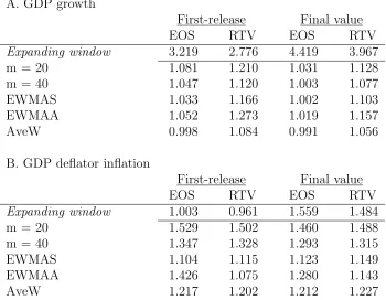
Table 6: Out-of-sample relative RMSFE values A. GDP growth

First-release Final value EOS RTV EOS RTV

Expanding window 3.219 2.776 4.419 3.967

m = 20 1.081 1.210 1.031 1.128 m = 40 1.047 1.120 1.003 1.077 EWMAS 1.033 1.166 1.002 1.103 EWMAA 1.052 1.273 1.019 1.157 AveW 0.998 1.084 0.991 1.056 B. GDP deflator inflation

First-release Final value EOS RTV EOS RTV

Expanding window 1.003 0.961 1.559 1.484

m = 20 1.529 1.502 1.460 1.488 m = 40 1.347 1.328 1.293 1.315 EWMAS 1.104 1.115 1.123 1.149 EWMAA 1.426 1.075 1.280 1.143 AveW 1.217 1.202 1.212 1.227

Notes: Forecasting periods for real GDP growth and GDP deflator inflation are 2008:Q4– 2011:Q1 and 1982:Q2–1984:Q3, respectively. The first row in each panel shows the root mean squared forecast error for the expanding window estimator. Subsequent rows show the ratio of the RMSFE of a candidate window selection method to the RMSFE of the benchmark expanding window estimator. Forecasts of final values are bias corrected first-release forecasts.

The correction is based on the sample mean of the difference between the final values,yt_t+15,

and the first-release values,ytt+1, calculated with data up to the forecast origin. We usey t+16

t+1 as true values for GDP deflator inflation and the vintage 2012:Q2 values as true values for real GDP growth.

the RMSFE value of the benchmark expanding window estimator. The subsequent rows

show the RMSFE of a candidate window selection method relative to the RMSFE of the

benchmark. Forecasts of final values are bias corrected first-release forecasts. The correction

is based on the sample mean of the difference between the final values, yt_t+15, and the

first-release values, y_tt+1, calculated with data up to the forecast origin. We use y_tt+16₊₁ as true

values for inflation and the vintage 2012:Q2 values as true values for real GDP growth. To

ensure that our empirical results are comparable to our Monte Carlo results, we consider an

AR(1) specification.5

The AveW and the expanding window estimator produce the most accurate real GDP

5

We also considered AR(2) and AR(4) models. The results for these specifications are qualitatively similar to those presented in Table 6.

forecasts. When we use the EOS approach, the AveW method does marginally better than

the expanding window estimator. By contrast, the expanding window estimator turns out

to be the best method when the RTV approach is used. For the GDP deflator inflation,

the expanding window estimator is overwhelmingly the best estimation window method. It

produces the most accurate forecasts in each of the four dependent variable/vintage approach

combinations considered here. The differences in the forecasting abilities are very large. The

relative RMSFE values range between 1.075 and 1.529, indicating that the alternative window

selection methods produce 7.5-52.9 percent larger forecast errors than the expanding window

benchmark.

Our simulation results are useful in explaining why it is difficult to outperform the

ex-panding window estimator after a recent break. For example, if the break only affects the

innovation variance,σ2, our simulation results indicate that the expanding window estimator

produces the most accurate forecasts. The two breaks considered here most likely caused

changes in the innovation variance. In particular, the results in the literature indicate that

the variance of the inflation series has reduced substantially since the early 1980s. This

would explain why none of the alternative methods systematically improve upon the

expand-ing window benchmark. Another reason for the good performance of the expandexpand-ing window

estimator lies in the fact that the means of the series have declined after the breaks (at least

temporarily). The simulation results show that when the mean declines after the break, the

expanding window estimator performs well relative to the alternatives (see experiments 3

and 9). Note also that the differences in the relative predictive abilities are larger for the

GDP deflator inflation. As discussed in Section 2, revisions to the GDP deflator inflation are

mainly noise, whereas those to the GDP are mainly news (see, e.g., Clements and Galv˜ao,

2013). Thus, our results suggest that the differences in the relative predictive abilities are

larger when the revisions reduce noise. In addition, our results indicate that, in general, the

expanding window method performs better when the first-release values are the ones to be

forecast. These two findings are consistent with our simulation results in Tables 2–5.

The rolling window methods and the EWMAA method perform poorly in our empirical

sub-stantially worse than those produced by the expanding window benchmark. These empirical

findings are in line with our Monte Carlo simulations. Indeed, our simulation results suggest

that these methods rarely outperform the expanding window estimator.

The results in Table 6 also indicate that one key determinant of the forecasting

per-formance is the choice of how to use the real-time data to estimate the parameters of the

forecasting model. A substantial amount of the literature on real-time forecasting uses the

EOS approach. In our empirical examples, the RTV approach produces more accurate

fore-casts after a recent break regardless of whether we consider forecasting the real GDP or the

GDP deflator inflation. We find that the RTV approach yields improvements of 4.8%–13.8%

over the EOS approach.

6.

Conclusions

This paper analyzes the forecasting performance of various window selection methods after

a recent break when the data are subject to revision. Several practical recommendations

for choosing the estimation window emerge from our analysis. First, our Monte Carlo and

empirical results suggest that the expanding window method usually provides the most

ac-curate forecasts after a recent break. It performs well regardless of whether the revisions add

news or reduce noise, or whether we forecast the first-release or the final values. Thus, the

evidence in favor of the expanding window estimator seems well established. Second, we find

that rolling windows perform the worst of all the methods. They never produce the most

accurate forecasts in any of the cases considered here. Furthermore, they rarely improve

upon the expanding window estimator. This is an important result because rolling windows

are used extensively in the literature. In short, our results suggest that the use of rolling

windows should be rethought, at least when making forecasts after a recent break. Third, our

results imply that whether the revisions add news or reduce noise does not matter much for

the relative ranking of the alternative window selection methods. Finally, no clear ranking

between the EOS and RTV vintage approaches emerges. In general, our Monte Carlo results

suggest that the RTV approach produces more accurate forecasts when the revisions add

news, whereas the EOS approach yields more reliable forecasts when the revisions reduce

noise. The RTV approach performs particularly well in our empirical examples.

Our results could be extended in several ways. We have considered only cases where

the autoregressive process has been subject to a single, recent break. In practice, however,

autoregressive processes are likely to be subject to multiple breaks. Therefore, analyzing

the forecasting performance in the presence of multiple breaks might be a fruitful area for

future research. In addition, our statistical framework neglects some important features of

the actual data revision process, including time variations in the revision mean and variance.

Incorporating these features into the statistical framework may lead to a better understanding

of the relative forecasting accuracy of alternative window selection methods in the presence

Appendix A

In this Appendix, we derive formulas for the means and variances of the first-release data,

yt_t+1, and final data, ˜yt . Recall that ˜yt = ρ+Pil=1µvi+βy˜t−1+ση1t+

Pl

i=1σviη2t,i and

yt_t+1 = ˜yt −Pli=1µvi −Pli=1σviη2t,i −µε1 +σε1η3t,1. Both y

t+1

t and ˜yt are (covariance)

stationary processes. We set l = 14, so that we observe 14 different estimates of yt before

the true value, ˜yt, is observed. The expected value of ˜ytis

E(˜yt) =µy˜=

ρ+

l

X

i=1

µvi

1−β .

Therefore, the expected value ofyt_t+1 is

E(yt_t+1) =E(˜yt)− l

X

i=1

µvi−µε1

=

ρ+β

l

X

i=1

µvi

1−β −µε1.

If the revisions are pure news, the expected values of the first-release and final data are

E(˜yt) =

ρ+

l

X

i=1

µvi

1−β and E(y

t+1

t ) =

ρ+β

l

X

i=1

µvi

1−β .

If the revisions are pure noise, the expected values of the first-release and final data are

E(˜yt) =

ρ

1−β and E(y

t+1

t ) =

ρ

1−β −µε1.

The revisions are defined by rti = ytt+1+i −y t+i

t , for i = 1,...,l. For example, the first

revision at time t is equal to r1

t = ytt+2 −ytt+1, i.e., the difference between the

second-release value and the first-second-release value. Equations (1), (2), and (3) imply that yt_t+1 =

ρ+βy˜t−1+ση1t−µε1+σε1η3t,1 and y

t+2

t =ρ+µv1+βy˜t−1+ση1t+σv1η2t,1−µε2+σε2η3t,2.

Hence,

r1t =ytt+2−y t+1

t =µv1 +σv1η2t,1−µε2 +σε2η3t,2+µε1 −σε1η3t,1.

Following Clements and Galv˜ao (2013), we assume that the first and the fifth revisions have

non-zero mean. To be more specific, we assume that the means of the first and fifth revisions

are, respectively,δ and δ/2 times the mean of the first-release data. In what follows, we set

δ= 0.04. Our assumptions imply that for news revisions,

E(r1_t) =µv1

E(r2_t) =µv2

.. .

E(r_t14) =µv14,

so that µv2 = µv3 = µv4 = µv6 = ... = µv14 = 0, E(r 1

t) = µv1 and E(r 5

t) = µv5. Setting

E(r_t1) =δE(y_tt+1) yields

µv1 =δ

ρ+β

l

X

i=1

µvi

1−β .

Using the fact that E(r_t1) = 2E(r5_t), i.e.,µv1 = 2µv5, we can expressµv1 and µv5 as

µv1 =

δρ

1−(1 + 1.5δ)β and µv5 =

µv1

2 .

and our assumptions imply that

E(r1t) =−µε2+µε1 =δE(y

t+1

t )

E(r2t) =−µε3+µε2 = 0

E(r3_t) =−µε4+µε3 = 0

E(r4_t) =−µε5+µε4 = 0

E(r5_t) =−µε6+µε5 =

δ

2E(y

t+1

t )

E(r6_t) =−µε7+µε6 = 0

.. .

E(r_t13) =−µε14+µε13 = 0

E(r_t14) =µε14 = 0.

Revisions 6–14 have zero mean, which implies thatµε6 =µε7 =...=µε13 =µε14 = 0. Because

µε6 = 0, µε5 equals

δ

2E(y

t+1

t ). This finding implies thatµε2 =µε3 =µε4 =µε5 =

δ

2E(y

t+1

t ).

Finally, we find thatµε1 = 3δ

2E(y

t+1

t ). So, if the revisions are pure noise,

µε1 =

1.5 (1 + 1.5δ)

δρ

(1−β), µε2 =...=µε5 =

δ

2(1 + 1.5δ)

ρ

(1−β), µε6 =...=µε14 = 0.

Next, we derive the variance of ˜yt. The true values can be expressed as follows

(˜yt−µy˜) =β(˜yt−1−µy˜) +ση1,t+

l

X

i=1

σviη2t,i, (7)

where µ˜y denotes the expected value of ˜yt. The variance of ˜y can be found by multiplying

(7) by (˜yt−µy˜) and taking expectations:

E(˜yt−µy˜)2=βE[(˜yt−µy˜)(˜yt−1−µy˜)]+E[(˜yt−µy˜)ση1t]+E

"

(˜yt−µy˜)

l

X

i=1

σviη2t,i

#

. (8)

Note that

E[(˜yt−µy˜)ση1t] =σ2E(η21t) =σ2 and

E

"

(˜yt−µy˜)

l

X

i=1

σviη2t,i

#

=

l

X

i=1

σ_vi2E(η₂2_t,i) =

l

X

i=1

σ2_vi.

Thus, (8) can be rewritten as

γ0 =βφ1γ0+σ2+

l

X

i=1

σ_vi2, (9)

whereγ0denotes the variance and φ1 the first autocorrelation coefficient. Using the fact that

for an AR(1) process,φ1 =β, we have

γ0 =

σ2+

l

X

i=1

σv2i

1−β2 .

The variance ofy_tt+1 can be derived as follows

var(yt_t+1) =var(˜yt− l

X

i=1

µvi− l

X

i=1

σviη2t,i−µε1+σε1η3t,1)

var(yt_t+1) =var(˜yt) + l

X

i=1

σ_vi2var(η2t,i) +σε21var(η3t,1)−2

l

X

i=1

σvicov(˜yt, η2t,i)

+2σε1cov(˜yt, η3t,1)−2

l

X

i=1

σviσε1cov(η2t,i, η3t,1).

Becausecov(˜yt, η2t,i) = l

X

i=1

σvi,cov(˜yt, η3t,1) = 0, andcov(η2t,i, η3t,1) = 0, we have

var(yt_t+1) =var(˜yt) + l

X

i=1

σ_vi2 +σ_ε2₁ −2

l

X

i=1

=

σ2+

l

X

i=1

σ_vi2

1−β2 −

l

X

i=1

σ_vi2 +σ_ε2₁

=

σ2+β2

l

X

i=1

σ_vi2

1−β2 +σ 2

ε1.

Therefore, when the revisions are pure news, we have

σ2_yt+1

t

=

σ2+β2

l

X

i=1

σv2i

1−β2 .

When the revisions are pure noise, the variance is

σ2_yt+1

t

= σ

2

1−β2 +σ 2

ε1.

Next, we derive the variances of the data revisions. Let σ_ri2 (for i = 1,...,l) denote the

variance of the ith revision. The variance of the first revision is

var(r_t1) =var(y_tt+2−y_tt+1) =var(µv1 +σv1η2t,1−µε2 +σε2η3t,2+µε1−σε1η3t,1).

If the revisions are pure news, var(r1_t) = σ_r2₁ = var(µv1 +σv1η2t,1) = σ 2

v1var(η2t,1) = σ 2

v1.

If the revisions are pure noise, var(r_t1) = σ_r2₁ = var(−µε2 +σε2η3t,2 +µε1 −σε1η3t,1) =

σ2

ε2var(η3t,2) +σ 2

ε1var(η3t,1) =σ 2

ε2+σ 2

ε1.

We set σr1 = ασ_yt+1

t , where α denotes the ratio of the standard deviation of the first

revision to the standard deviation of the first-release data. Furthermore, we assume that

σr2,...,r13 =

α

2σytt+1 and that σr14 = α

4σytt+1. In what follows, we set α = 0.4. Thus, the

variance of the first revision, when the revisions are pure news, can be found by solving the

equation

σ2v1 =α 2

σ2+β2

l

X

i=1

σ_vi2

1−β2 .

Note that 1/4σv21 = σ 2

v2 = ... = σ 2

v13 and 1/16σ 2

v1 = σ 2

v14. This implies that

Pl

i=1σv2i =

4.0625σ2

v1. Using this fact we can express the variance of the first revision as

σ2_v1 =α2σ

2_{+ 4.0625β}2_σ2

v1

1−β2 .

After some algebra, we find that

σ2_v1 = α

2_σ2

1−(1 + 4.0625α2_)β2.

So, the formulas for the standard deviations are

σv1 =

s

α2_σ2

1−(1 + 4.0625α2_)β2, σv2 =...=σv13 =σv1/2, σv14 =σv1/4.

Next, we consider noise revisions. We have

σ_r2₁ =σ_ε2₂ +σ_ε2₁

σ_r2₂ =σ_ε2₃ +σ_ε2₂

.. .

σ2_r13 =σ_ε2₁₄+σ2_ε13

σ2r14 =σ 2

ε14.

Using the fact that revisions 2–13 have equal variance, we find that

σ2_ε2 =σ2_ε4 =...=σ_ε2₁₂ =σ_ε2₁₄ and σ2_ε3 =σ_ε2₅ =...=σ_ε2₁₃.

Note thatσr13 =α/2σ_yt+1

t and σr14 =α/4σy t+1

t , implying that 4σ

2

r14 =σ 2

r13. Therefore,

4σ_ε2₁₄ =σ2_ε14+σ_ε2₁₃,

which in turn implies that σ2_ε13 = 3σ_ε2₁₄. Plugging σ_ε2₂ = ...=σ_ε2₁₄ = (α₄)2h₁σ2 −β2 +σ

2

ε1

i

σε22+σ 2

ε1 =α 2_σ2

yt_t+1 yields

α2

16

σ2

1−β2 +σ 2

ε1

+σ_ε2₁ =α2

σ2

1−β2 +σ 2

ε1

.

After some algebra, we find that

σ2_ε1 = 15α

2

16−15α2

σ2

1−β2.

So, the formulas for the standard deviations are

σε1 =

s

15α2

16−15α2

σ2

1−β2,

σε2 =σε4 =...=σε14 =

s α

4

2 16

16−15α2

σ2

1−β2,

σε3 =σε5 =...=σε13 =

s

3α 4

2 16

16−15α2

σ2

1−β2.

Appendix B

Means and standard deviations

News

Experiment E(˜y1t) E(˜y2t) E(y1t+1t ) E(y t+1

2t ) σ˜y1t σy˜2t σy1t+1t

σ y2t+1t

1 2.255 2.255 2.128 2.128 2.514 2.514 1.957 1.957

2 2.255 5.171 2.128 4.878 2.514 7.187 1.957 5.595

3 2.255 1.442 2.128 1.361 2.514 2.035 1.957 1.584

4 1.442 5.171 1.361 4.878 2.035 7.187 1.584 5.595

5 5.171 1.442 4.878 1.361 7.187 2.035 5.595 1.584

6 2.255 2.255 2.128 2.128 2.514 7.541 1.957 5.871

7 2.255 2.255 2.128 2.128 2.514 0.838 1.957 0.652

8 2.255 3.383 2.128 3.191 2.514 2.514 1.957 1.957

9 2.255 1.128 2.128 1.064 2.514 2.514 1.957 1.957

Noise

Experiment E(˜y1t) E(˜y2t) E(y1t+1t ) E(y t+1

2t ) σ˜y1t σy˜2t σy₁t+1_t σy₂t+1_t

1 2.000 2.000 1.887 1.887 1.732 1.732 1.879 1.879

2 2.000 4.000 1.887 3.774 1.732 2.268 1.879 2.460

3 2.000 1.333 1.887 1.258 1.732 1.549 1.879 1.680

4 1.333 4.000 1.258 3.774 1.549 2.268 1.680 2.460

5 4.000 1.333 3.774 1.258 2.268 1.549 2.460 1.680

6 2.000 2.000 1.887 1.887 1.732 5.196 1.879 5.636

7 2.000 2.000 1.887 1.887 1.732 0.577 1.879 0.626

8 2.000 3.000 1.887 2.830 1.732 1.732 1.879 1.879

References

Altissimo, F. and Corradi, V. (2003). Strong rules for detecting the number of breaks in a

time series.Journal of Econometrics, 117, 207–244.

Andrews, D. W. K. (1993). Tests for parameter instability and structural change with

unknown change point.Econometrica, 61, 821–856.

Andrews, D. W. K., Lee, I. and Ploberger, W. (1996). Optimal changepoint tests for normal

linear regression.Journal of Econometrics, 70, 9–38.

Aruoba, S. B. (2008). Data revisions are not well-behaved.Journal of Money, Credit and

Banking, 40, 319–340.

Bai, J. and Perron, P. (1998). Estimating and testing linear models with multiple structural

changes.Econometrica, 66, 47–78.

Bai, J. and Perron, P. (2003). Computation and analysis of multiple structural change

models.Journal of Applied Econometrics, 18, 1–22.

Clements, M. P. and Galv˜ao, A. B. (2013). Real-time forecasting of inflation and output

growth with autoregressive models in the presence of data revisions.Journal of Applied

Econometrics, 28, 458–477.

Clements, M. P. and Hendry, D. F. (1998). Forecasting economic time series. Cambridge

University Press: Cambridge.

Clements, M. P. and Hendry, D. F. (2006). Forecasting with breaks. In Elliott, G., Granger,

C. W. J. and Timmermann, A. (Eds.),Handbook of Economic Forecasting, Vol. 1.

Amsterdam: Elsevier, 605–657.

Croushore, D. (2011). Frontiers of real-time data analysis.Journal of Economic Literature,

49, 72–100.

Eklund, J., Kapetanios, G. and Price, S. (2013). Robust forecast methods and monitoring

during structural change.Manchester School, 81, 3–27.

Giacomini, R. and White, H. (2006). Tests of conditional predictive ability.Econometrica,

74, 1545–1578.

Giraitis, L., Kapetanios, G. and Price, S. (2013). Adaptive forecasting in the presence of

recent and ongoing structural change.Journal of Econometrics, 177, 153–170.

Jacobs, J. P. A. M. and van Norden, S. (2011). Modeling data revisions: measurement error

and dynamics of “true” values.Journal of Econometrics, 161, 101–109.

Koenig, E. F., Dolmas, S. and Piger, J. (2003). The use and abuse of real-time data in

economic forecasting.Review of Economics and Statistics, 85, 618–628.

Mankiw, N. G. and Shapiro, M. D. (1986). News or noise: an analysis of GNP revisions.

Survey of Current Business, 66, 20–25.

McConnell, M. M. and Perez-Quiros, G. (2000). Output fluctuations in the United States:

what has changed since the early 1980’s? American Economic Review, 90, 1464–1476.

Pesaran, M. H. and Pick, A. (2011). Forecast combination across estimation windows.

Journal of Business and Economic Statistics, 29, 307–318.

Pesaran, M. H., Pick, A. and Pranovich, M. (2013). Optimal forecasts in the presence of

structural breaks.Journal of Econometrics, 177, 134–152.

Pe