Transmission Electron Microscopy Study on the Grain Boundaries and Magnetic Domains in Nd–Fe–B Based Magnets

whereas reversal was occurred simultaneously in different grains in the as-sintered specimen. [doi:10.2320/matertrans.M2009277]

(Received August 7, 2009; Accepted November 11, 2009; Published January 25, 2010)

Keywords: electron holography, Lorentz microscopy, permanent magnet, coercivity, domain wall

1. Introduction

Since its discovery in the 1980s,1)_{the Nd–Fe–B system has} attracted considerable interest from researchers due to its excellent performance as a permanent magnet. For example, the sintered Nd2Fe14B compound has the highest maximum

energy product among the permanent magnets developed so far.2) Such high performance has led to it being used in several industrial applications, including hybrid vehicle motors, computer disk drives, and magnetic resonance imagers.3)_{For such applications it is desirable to miniaturize} the magnetic components, but this requires further improving the performance of magnets. Thus, researchers are greatly interested in the microscopic mechanisms that give rise to the excellent magnetic properties in the Nd–Fe–B system. The effect of heat treatment on the microstructure, the coercivity, and the magnetization reversal is one important issue, which we focus on in this study.

There are two crystalline phases that are of practical importance to the study of Nd–Fe–B magnets. The first one is a hard magnetic phase, Nd2Fe14B, which has a relatively high

magnetocrystalline anisotropy of the order of106J/m3.4)The Nd2Fe14B phase has a space group ofP42=mnm.5)The lattice

parameters of the tetragonal unit cell area¼0:880nm and c¼1:221nm. The other phase is referred to as the Nd-rich phase and is a nonmagnetic phase.6,7)_{Typically, the Nd-rich} phase exists as a thin film coating on grains of the Nd2Fe14B

phase. An electron microscopy study by Shinba et al.7) revealed that the Nd-rich phase is a type of neodymium oxide. They also found that the Nd-rich phase is amorphous at thin film thicknesses (i.e., a few nanometers), whereas it is crystalline in thicker portions of the same film. Ramesh

et al.8)_{found that the crystalline Nd-rich phase has a} face-centered cubic unit cell with an approximate lattice param-eter a¼0:52nm, but Shinba et al.7) proposed large cubic super cells witha¼1:1nm.

Importantly, the coercivity of Nd–Fe–B magnets is influenced by post-sintering heat treatment.9–11)This implies

that there is a close relationship between the microstructure and the magnetic properties. Several different mechanisms have been proposed for the effect of heat treatment, including greater compositional uniformity in the Nd2Fe14B

phase,12)_{reduced internal stress in the Nd}

2Fe14B phase,12–16)

greater magnetic separation between adjacent Nd2Fe14B

grains,1,10,11,17) and greater magnetocrystalline anisotropy (Nd2Fe14B phase) in the vicinity of grain boundaries.18,19)

In addition, the morphology of the grain boundaries is an important factor that also requires careful investigation. For example, the roughness of the grain boundaries, which can be controlled by post-sintering heat treatment, can affect nucleation of reverse magnetic domains. However, despite intensive study, the underlying mechanism for the improve-ment in the coercivity is still under debate. Transmission electron microscopy (TEM) is useful for gaining a deeper understanding of the effect of post-sintering heat treatment on the coercivity, since it allows both the magnetic and crystallographic microstructures in Nd–Fe–B magnets to be observed. This is the motivation behind this study.

The purpose of the present study is to obtain in-depth information about the effect of post-sintering heat treatment on the magnetic properties in Nd–Fe–B based permanent magnets. To this end, we carefully observed the boundary structures in both as-sintered (i.e., without post-sintering heat treatment) and heat-treated specimens by TEM. Furthermore, we investigated the magnetization reversal processes in both specimens by observing various stages of the remanent state with the aid of electron holography, i.e., by performing

ex situobservations of magnetization reversal.

2. Experimental Procedure

of the applied field. Two types of specimens, samples A and B, were prepared in this study. Sample A was in the as-sintered state and had an intrinsic coercivity of 1170.8 kA/m. Sample B was subjected to post-sintering heat treatment at 853 K for 3.6 ks. It had an intrinsic coercivity of 1705.3 kA/m, which is higher than that of sample A. Thin foil specimens for TEM observations were prepared using a focused ion beam (FIB) system (JEM-9310FIB). These specimens (4:550:1mm) were obtained by slicing the pellet such that the foil planes contained the easy magnet-ization axis. The thin foil specimens were supported on carbon-coated copper grids. Crystallographic microstructures were observed by using transmission electron microscopes (JEM-2010 and JEM-ARM1250). In addition to the conventional TEM observations, we also acquired a high-angle annular dark-field scanning TEM (HAADF-STEM) images to reveal the grain boundary structure: the latter technique is useful for phase identifications since the image contrast is sensitive to the elemental number of constituents. Chemical analysis for regions near the grain boundaries was conducted by energy-dispersive X-ray spectroscopy (EDS) using a field-emission transmission electron microscope (JEM-2100F). Magnetic domain structures were studied by electron holography20) _{using another electron microscope} (JEM-3000F), which was equipped with a magnetically shielded objective lens so that the magnetic field at the specimen position was negligible due to the shielding. To obtain information about magnetization reversal, magnetic fields were applied to the thin foil specimens by using an electromagnet outside the electron microscope. Computer simulation of the magnetic flux distribution was performed by using commercial software (JMAG Studio, version 8.4).

3. Results

3.1 Analysis of crystallographic microstructure

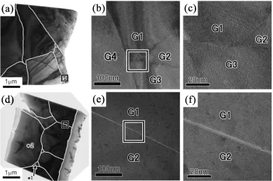
We first compared the crystallographic microstructures of samples A and B. The bright-field image in Fig. 1(a) shows the microstructure of sample A. White lines trace the grain boundaries. Large grains, with sizes of the order of 1mm, represent the Nd2Fe14B phase; phase identification was

carried out by electron diffraction (results not shown here). Figure 1(b) shows a magnified image of the area enclosed in the square in Fig. 1(a); the four grains in the field of view are labeled G1, G2, G3, and G4. The magnified image in Fig. 1(b) shows that the grain boundaries (the dark regions) are not very smooth, but rather they meander to some extent. Figure 1(c) shows a lattice image that was acquired from the area enclosed in the square in Fig. 1(b). It demonstrates that the lattice fringes are discontinuous at the grain boundaries. The width of the grain boundary was estimated to be approximately 2 nm from the projected image in Fig. 1(c). There was no lattice fringe that indicated a crystalline state within the grain boundaries.

A similar analysis was conducted on sample B (see Figs. 1(d)–(f)). The light gray area on the left edge of the specimen represents a deposited carbon layer (Fig. 1(d)), while the area at the right edge represents a portion that had been damaged by FIB polishing. The grain size of the Nd2Fe14B phase is comparable with that of sample A.

Figure 1(e), which is a magnified image of the area enclosed by the square in Fig. 1(d), shows that the smoothness of the grain boundaries is improved in sample B. The smoothness of the boundary is clearer in the lattice image shown in Fig. 1(f), which is an enlarged image of Fig. 1(e). Lattice fringes in

Fig. 1 Boundary structures in sample A (upper panels) and sample B (lower panels). (a) Bright-field image of an as-sintered specimen (sample A). (b) Enlarged image of the area enclosed in the square in (a). (c) Lattice image observed in the area enclosed by a square in (b). (d) Bright-field image of a specimen subjected to post-sintering heat treatment (sample B). (e) Enlarged image of the area enclosed by a square in (d). (f) Lattice image of the area enclosed by a square in (e).

grain G1 are absent due to significant misalignment with the crystallographic zone axis. The width of the grain boundaries was approximately 2 nm (see Fig. 1(f)), which is essentially the same as that of sample A.

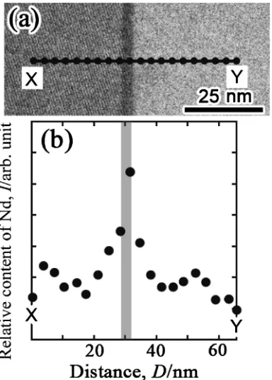
To identify the phases in the grain boundaries and at triple junctions, we performed EDS analysis with a fine electron probe whose diameter was approximately 1 nm. Figure 2(a) shows a HAADF-STEM image of sample B. There are two grains of the Nd2Fe14B phase, on the left and right sides of

the field of view. The lattice fringe in the right grain is absent due to tilting of the zone axis. The central dark portion, which is approximately 3 nm wide, represents a grain boundary. The intensity of the Nd-L line (5.23 keV) was measured along the line X-Y in Fig. 2(a). The dark dots in Fig. 2(a) indicate the points at which spectra were acquired. The results are plotted in Fig. 2(b). The relative content of Nd is greater in the grain boundary than outside it. Thus, it is reasonable to conclude that the grain boundaries consist of the Nd-rich phase. Although brightness of a HAADF-STEM image tends to increase with increasing atomic number of constituents, the boundary portion (Nd-rich phase) in Fig. 2(a) is particularly dark. This observation appears to be explained by a reduced specimen thickness in the boundary area—i.e., due to the difference in the etching rate during FIB polishing, the portion of boundaries may be thinner than that of grains. In addition, we should also consider a fact that the Nd-rich phase is a type of oxide, while the grains on the both sides are in a distinct metallic

phase (Nd2Fe14B phase) containing Nd and Fe.

Neverthe-less, the EDS analysis explicitly indicates the enhancement of Nd content in the vicinity of the grain boundary. The EDS analysis was conducted only for sample B. However, it is reasonable to consider that the boundaries in sample A are also in the Nd-rich phase, since the Nd-rich phase can be produced by the sintering process: in fact, several research groups mentioned about the Nd-rich phase in the grain boundaries in as-sintered specimens.4,7) _{We also acquired} spectra from points within a triple junction (sample B). For example, Fig. 3(a) shows a spectrum obtained from the portion of the triple junction indicated by asterisk 1 in Fig. 1(d). That spectrum should be compared with the one shown in Fig. 3(b), which was acquired from a grain of the Nd2Fe14B phase (asterisk 2 in Fig. 1(d)). The Cu-K line (8.05 keV) is due to the background signal from the copper grid. It is noted that signals from Fe are prominent in Fig. 3(b), whereas they are almost absent in Fig. 3(a). The major metallic element is likely to be Nd in the spectrum of Fig. 3(a). These observations indicate that the Nd-rich phase also exists at triple junctions. The results are consistent with those reported in previous studies.6,7)

3.2 c-axis direction in grains of Nd2Fe14B phase

The magnetic domain structure was investigated in the two specimens shown in Fig. 4(a) (sample A) and Fig. 4(b) (sample B). Sample B is the same specimen as that used for the microstructural analysis (Fig. 1(d)). Since the Nd–Fe–B system is a hard magnet, it is particularly important to determine the direction of the c-axis in each grain in the specimens. We here briefly explain how the arrows in Fig. 4 were determined, which indicate the direction of the c-axis (strictly speaking, the projection of the c-axis onto the foil plane), by referring to sample B. As mentioned in the previous section, a pellet of a Nd–Fe–B magnet was subjected to pressing in a uniaxial magnetic field to align

Fig. 2 Composition analysis of a grain boundary in sample B. (a) High-angle annular dark-field scanning TEM image of sample B. The central dark portion represents the grain boundary that separates grains in the Nd2Fe14B phase. (b) Plot of the relative content of Nd measured at the

points indicated by the closed circles in (a). The thick gray line represents the position of the grain boundary that is deduced from the image in (a). The symbols X and Y indicate the initial and final measurement points, respectively.

Fig. 3 Energy dispersive X-ray spectra acquired from (a) a grain boundary and (b) an interior portion of a grain in the Nd2Fe14B phase. The

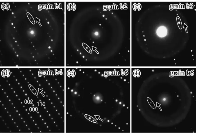
the c-axis of each grain with the direction of the applied field. In fact, an electron diffraction pattern (Fig. 5(d)) obtained from grain b4 demonstrates that the c-axis is approximately parallel to the foil plane; for this grain, the direction of the c-axis was determined straightforwardly, as indicated by the black arrow in Fig. 4(b). The other diffraction patterns in Figs. 5(a)–(c), (e), and (f) were obtained from grains b1, b2, b3, b5, and b6 in Fig. 4(b), respectively. These diffraction patterns were obtained using the same conditions of electron beam incidence as those used for Fig. 5(d). Therefore, the incident electron beam was not exactly parallel to the zone axes in grains b1, b2, b3, b5, and b6. Nevertheless, arrays of diffraction spots along thec_{-axis (such as those indicated by the ellipses in}

Fig. 5) are visible in the diffraction patterns. These arrays of diffraction spots were used to determine the trace of the c-axis (i.e., its projection onto the foil plane) in grains b1, b2,

b3, b5, and b6. The observations indicate that, as a result of applying a magnetic field during pressing, the orientation of thec-axis does not vary greatly between the grains, although it is difficult to accurately evaluate the magnitude of the orientational deviations in off-axis diffraction patterns. The same technique was applied to sample A to determine the trace of thec-axis, as shown in Fig. 4(a). Grains b7, b8, and b9 in Fig. 4(b) were identified to be the Nd-rich phase by EDS analysis.

3.3 Holography studies of the magnetization reversal process

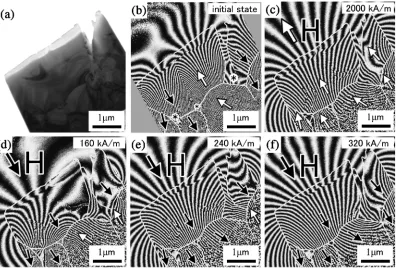
Figures 6 and 7 show reconstructed phase images (i.e., the results of electron holography) of samples A and B. Figure 6(a) shows a portion of sample A. The other panels in Fig. 6 show the magnetic flux distribution in this field of view. The observations (except for Fig. 6(b)) represent the

Fig. 4 Bright-field images of the specimens that were used for magnetic domain observations: (a) sample A, and (b) sample B. Symbols a1–a4 and b1–b9 represent crystallographic grains in each specimen. Black arrows indicate the direction of thec-axis (grains in the Nd2Fe14B phase) projected onto the foil plane.

Fig. 6 Ex situobservations of magnetization reversal in sample A. (a) Bright-field image showing the same region of the specimen as that in Fig. 4(a). (b)–(f) Reconstructed phase images observed in the same field of view as that in (a): (b) initial state, (c) remanent state after applying a magnetic field of 2000 kA/m, and (d)–(f) remanent states after applying magnetic fields of 160 kA/m, 240 kA/m, and 320 kA/m, respectively, in the opposite direction to that of (c). Small black and white arrows indicate the direction of thec-axis (easy magnetization axis) projected onto the foil plane. Large arrows labeled ‘‘H’’ indicate the direction of the applied magnetic field.

remanent states observed under several different experimen-tal conditions, as described below. Figure 6(b) shows a result for the initial state; i.e., holography was performed imme-diately after making the thin foil specimen. The contour lines represent the lines of magnetic flux. The white curves trace the specimen edge and the grain boundaries. The arrow in each grain indicates the in-plane component of magnetization vector. The direction of the arrow was determined by considering the flux lines, the sign (positive or negative) of the phase shift, and the trace of thec-axis (as shown in Fig. 4) which was examined after performing all the magnetic domain observations. Due to the effect of a stray magnetic field from the specimen, the magnetization vectors are not always parallel to the contours lines which represents the magnetic flux component projected along the incident electron beam: the effect of a stray magnetic field will be discussed in greater detail in the last part of this section, using both the experimental result and computer simulation. Despite the fact, the observations of electron holography provide useful information about the process of magnet-ization reversal as described below.

After obtaining the result shown in Fig. 6(b), the specimen was removed from the electron microscope and it was subjected to an external magnetic field (2000 kA/m) gen-erated by an electromagnet to magnetize the specimen. Figure 6(c) shows a flux map of the remanent state after applying a magnetic field of 2000 kA/m; the arrow labeled ‘‘H’’ indicates the direction of the applied magnetic field. The magnetization vectors are reversed compared with those in Fig. 6(b). Subsequently, to investigate the magnetization reversal process, magnetic fields were applied along the opposite direction and the remanent states were observed using the same technique. The results are shown in Figs. 6(d)–(f). When a magnetic field of 160 kA/m was applied along the black arrow labeled ‘‘H’’ (Fig. 6(d)), the remanent state remained unchanged. Magnetization reversal did not occur even by applying a higher magnetic field of 240 kA/m (see Fig. 6(e)). However, when a magnetic field of 320 kA/m was applied, the magnetization was reversed in most of the grains (see Fig. 6(f)). It appears likely that the magnetization reversal in sample A occurred immediately in several grains when a magnetic field was applied. Only one small grain at a corner of the specimen remained unchanged in Fig. 6(f). The reason why the magnetization in this grain remains the same is unclear. This small grain might be subject to a complex magnetic field due to the much larger volumes of the neighboring grains. Alternatively, the particular magnetization distribution might be stabilized by various crystallographic/microstructural factors.

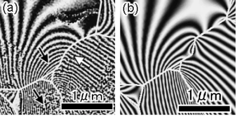
Magnetization reversal in sample B was examined by using the same method described above. Figure 7(a) shows a bright-field image of sample B (the same image as that shown in Fig. 4(b)) and Fig. 7(b) shows the magnetic flux distribu-tion in the initial state. The arrows in Fig. 7(b) represent magnetization vectors, which were determined by the method described above. Interestingly, the largest grain consists of two domains, whereas the other grains in the Nd2Fe14B phase

are single domains. The portions indicated by asterisks are the nonmagnetic Nd-rich phase. Figure 7(c) shows the remanent state observed after applying a magnetic field of

2000 kA/m along the direction indicated by the arrow labeled ‘‘H’’; in fact, the specimen was magnetized along this direction. When a magnetic field of 160 kA/m was applied in the opposite direction, the remanent state showed the pattern shown in Fig. 7(d). Relative to the result in Fig. 7(c), magnetization reversal has occurred in the four grains labeled by black arrows in Fig. 7(d). However, the other two grains (indicated by white arrows) in the Nd2Fe14B phase remained

unchanged at this stage. Increasing the applied magnetic field to 240 kA/m reversed the magnetization in one of the previously unchanged grains (see Fig. 7(e)). The last grain underwent magnetization reversal in a higher magnetic field of 320 kA/m (see Fig. 7(f)). An interesting observation is that magnetization reversal occurs in a stepwise manner in individual grains, rather than simultaneously (see Fig. 7). It appears likely that this behavior differs from that observed in sample A, although it is uneasy to directly compare the two specimens since they have dissimilar crystallographic grain configurations. In both specimens, magnetization reversal occurs in magnetic fields that were smaller than the values of the coercivity determined using bulk specimens. This discrepancy is presumably due to morphological factors (e.g., surface roughness, which might be introduced during FIB polishing) in the thin foil specimens used in these experiments. Thus, it is difficult to quantitatively discuss the phenomenon of magnetization reversal. Despite that, since both specimens were prepared by the same method, compar-ison of the holography results can provide useful information on the effect of heat treatment on the magnetization process. We here briefly discuss the interpretation of complicated magnetic flux maps, such as that shown in Fig. 7(d). As mentioned above, electron holography is capable of visual-izing the in-plane component of the magnetic flux. For example, when a simple closure domain is formed within a thin film (i.e., the magnetic flux exists mostly inside the film), the contour lines intimate the magnetization distribu-tion. However, with a head-to-head (or tail-to-tail) config-uration of magnetic domains, such as that shown in Fig. 7(d), the out-of-plane component of the magnetic flux (generated by the magnetic charges that are produced) is not negligible. Consequently, the observed flux map (i.e., the projected flux pattern) becomes more complicated, and the contour lines are no longer parallel to the magnetization vectors. Computer simulations will be useful for analyzing such cases. For example, Fig. 8(a) shows the central portion of the image in Fig. 7(d); the arrows in the figure correspond to the trace of thec-axis (i.e., the easy magnetization axis) in each grain of the Nd2Fe14B phase, as determined by electron

diffraction. Using a model specimen that has a grain configuration almost identical to that shown in Fig. 7(a) and magnetization vectors aligned parallel to the c-axis (assumed to be in-plane) in each grain, we calculated the three-dimensional magnetic flux distribution and the re-sultant phase shift of the electron wave. The calculated phase shift is plotted as a contour map in Fig. 8(b), which can be compared with the experimental results in Fig. 8(a). Reasonable agreement was obtained between Figs. 8(a) and (b). Thus, simulations appear to be useful for analyzing the remanent state which shows a complicated flux pattern as shown in Fig. 8(a).

4. Discussion

As demonstrated in Fig. 1, the boundary structures of samples A and B appear to be different. The grain boundaries were not very smooth (actually, they were meandering when observed by high-resolution electron microscopy) in the as-sintered state, but the smoothness was improved by the post-sintering annealing at 853 K for 3.6 ks. Such a microstruc-tural factor can influence the coercivity; for example, roughness in the grain boundary may assist nucleation of a reverse magnetic domain due to an increase in the demagnet-ization energy. In fact, the coercivity of a Nd–Fe–B magnet is thought to be dominated by the nucleation process of reverse magnetic domains.18)Thus, it appears reasonable to conclude that the greater smoothness of the surface caused by post-sintering heat treatment is one factor that influences the coercivity. On the other hand, there appear to be other factors that affect the coercivity. For example, one probable mechanism is a local reduction in the magnetocrystalline anisotropy near grain boundaries.18,19) _{Specifically, the} anisotropy in the Nd2Fe14B phase may be somewhat

degraded near the grain boundaries due to chemical processes that occur during sintering at high temperatures. The post-sintering heat treatment may reverse such spatial inhomoge-neity. To investigate the effect of inhomogeneity, we acquired an intensity profile of the Nd-L line across the grain boundary using a specimen that had been subjected to post-sintering heat treatment (see Fig. 2). The Nd content might be enhanced slightly in the vicinity of the boundary relative to that at the two terminal positions. However, the experimental accuracy was not sufficiently high to allow us to be conclusive regarding the inhomogeneity; note the fluctua-tions in the spectrum of Fig. 2(b). In the future, we intend to collect spectra with higher accuracy.

We have already pointed out the distinct behaviors of samples A and B with respect to theex situobservations of the magnetization reversal shown in Figs. 6 and 7. In the as-sintered specimen, magnetization reversal appears to occur simultaneously in different grains when a magnetic field is applied. In contrast, in the specimen subjected to heat treatment, magnetization reversal occurred in a stepwise manner in individual grains; in other words, magnetization reversal occurred in some grains at lower applied fields than other grains (see Fig. 7). Several researchers have pointed

heat treatment on the coercivity. The results are summarized as follows:

(1) In as-sintered specimens, high-resolution TEM observa-tions revealed that grain boundaries were not very smooth; they appeared to be meandering. The width of the boundaries was approximately 2 nm. In contrast, the smoothness of the grain boundaries was improved by post-sintering heat treat-ment at 853 K for 3.6 ks. The boundary width in the specimen subjected to the post-sintering heat treatment was compara-ble with that of the as-sintered specimen.

(2) EDS studies demonstrated that the grain boundaries consisted of the Nd-rich phase. In the high-resolution TEM images, there was no lattice fringe that indicated a crystalline state of the Nd-rich phase within narrow grain boundaries. The Nd-rich phase was also observed at triple junctions. (3) Ex situ observations of magnetization reversal were conducted by observing the magnetic domain structures in the remanent states by electron holography. In the as-sintered specimen, magnetization reversal occurred simultaneously in different grains on applying a magnetic field. However, in the specimen subjected to heat treatment, the magnetization reversal occurred in a stepwise manner in individual grains. This observation may shed light on understanding the effect of heat treatment on the magnetic separation between neighboring grains in the Nd2Fe14B phase.

Acknowledgements

This study was partly supported by Grants-in-Aid for Scientific Research (S) and (B) from the Japan Society for the Promotion of Science.

REFERENCES

1) M. Sagawa, S. Fujiwara, N. Togawa, H. Yamamoto and Y. Matuura: J. Appl. Phys.55(1984) 2083–2087.

2) J. F. Herbst: Rev. Mod. Phys.63(1991) 819–898.

3) K. H. J. Buschow:Ferromagnetic Materials, E. P. Wohlfarth and K. H. Buschow ed. (Elsevier, New York, 1988).

4) J. Fidler, D. Suess and T. Schrefl: Handbook of Magnetism, H. Kronmu¨ller and S. Parkin ed. (John Wiley & Sons Ltd., West Sussex, 2007).

5) J. F. Herbst, J. J. Croat, F. E. Pinkerton and W. B. Yelon: Phys. Rev. B

29(1984) 4176–4178.

6) J. Fidler: IEEE Trans. Magn.MAG-23(1987) 2106–2108.

7) Y. Shinba, T. J. Konno, K. Ishikawa, K. Hiraga and M. Sagawa: J. Appl. Phys.97(2005) 053504(1)–053504(8).

Homma: J. Magn. Magn. Mater.54–57(1986) 563–566.

9) M. Tokunaga, N. Meguro, M. Endo, S. Tanigawa and H. Harada: IEEE Trans. Magn.MAG-21(1985) 1964–1966.

10) G. Schneider, E.-T. Heing, F. P. Missel and G. Petzow: Z. Metallkd.81

(1990) 322–329.

11) F. Vial, F. Joly, E. Nevalainen, M. Sagawa, K. Hiraga and K. T. Park: J. Magn. Magn. Mater.242–245(2002) 1329–1334.

12) S. Szymura, A. A. Lukin, A. A. Zhuravlyev, M. C. Margaryyan, Y. M. Rabinovich and H. Bala: Phys. Status Solid. A174(1999) 513–519. 13) D. Eckert, D. Hinz, A. Handstein and J. Schneider: Phys. Status Solid.

A101(1987) 563–566.

14) P. A. Withey, E. J. Devlin, J. S. Abell and I. R. Harris: J. Magn. Magn.

Mater.80(1989) 67–70.

15) S. Hirosawa and Y. Tsubokawa: J. Magn. Magn. Mater.84(1990) 309–316.

16) Y. Tsubokawa, S. Hirosawa and R. Shimizu: Jpn. J. Appl. Phys. Part I

29(1990) 2737–2740.

17) G. F. Zhou, S. Y. Fu, X. K. Sun and Y. C. Chuang: Phys. Status Solid. A

121(1990) 257–264.

18) H. Kronmu¨ller, K.-D. Durst and M. Sagawa: J. Magn. Magn. Mater.74

(1988) 291–302.

19) H. Kronmu¨ller: Phys. Stat. Sol. (b)144(1987) 385–396.

20) D. Shindo and K. Oikawa: Analytical Electron Microscopy for Materials Science, (Springer Verlag, Tokyo, 2002).