Eutectic Growth Model Using Cell Automaton Method

Eutectic Growth Model Using Cell-Automaton Method

Toshiaki Himemiya

_{, Kenichi Ohsasa}

_{and Takahiro Saga}

2_{Graduate School of Engineering, Hokkaidou University, Sapporo 060-8628, Japan}

A cell-automaton model for a binary eutectic system has been developed. This study examines a Bridgeman-type temperature field with periodic boundary conditions. A stable operating range of lamellar spacings is obtained based on the parameters of the temperature field. The undercooling of the liquid phase ahead of the solid/liquid interface is also estimated in the calculations. The estimated lamellar spacings and undercoolings agree well with the predictions of the Jackson-Hunt model. [doi:10.2320/matertrans.M2009304]

(Received September 4, 2009; Accepted October 16, 2009; Published December 2, 2009)

Keywords: two-dimension, operating range, lamellar spacing, undercooling, Jackson-Hunt model

1. Introduction

Eutectic alloys are used widely in industrial materials such as cast iron (Fe-C), silmin (Al-Si) and soldering alloys. In addition to this use, the benefit of eutectic materials asin-situ

composites has attracted attentions. Namely, the minor phase acts as a physical function and the major phase supports the full strength of the material, compensating for the lack of strength of the minor part. Therefore, in order to develop a new functional structure as a composite material, control of the eutectic solidification would be a key technique.

Generally speaking, the methods of studying the formation of the structure of alloys can be divided in three ways. The first is the observation of structures and the measurement of specific parameters by experiment. This might be considered the starting point for all the scientific research. Secondly, the researchers try to construct analytical models which can predict the phenomena observed in the experiments. Using basic physical equations and presuming that a few effects of the thermodynamic ‘‘force’’ control the phenomena and that other effects can be regarded as negligible, a series of equations can be developed with suitable boundary/initial conditions. The solutions of the equations are obtained by an analytical method (or numerical calculations). The predic-tions of the analytical method, in turn, should be examined by experiments. As for the third method of study, numerical simulations have recently been developed. These include Monte Carlo simulations, phase-field methods, cell-autom-aton methods, etc. In numerical simulations, basic calculation rules are also formulated, but the effects of the rules are not considered prior to calculation. The effects are recognized after the calculations are performed.

In the field of study concerning eutectic growth, analytical models were explored after World War II.1–4)_{In these studies,}

the Jackson and Hunt (JH) model4) _{presented not only}

analytical solutions for the specific spacing and undercooling of the lamellar and rod-like regular eutectic growth, but also a hypothesis for the adjustment of the specific spacing. Irregular eutectic growth models have also been proposed.5,6)

The JH model has also been extended to rapid solidification condition.7) _{The methods of the JH model have also been}

applied to the growth of the three-phase structure with regular lamellar, rod + hexagon and semi-regular brick-type mor-phologies.8)_{In 1994, J. A. Spittle and S. G. R. Brown studied}

a 3-D cellular automaton model of coupled growth in two-component systems.9) _{They obtained lamellar structures in}

undercooled two component melts using a simple algorithm. In this work, we wish to compare the results of a 2-D cell-automaton model with those of the JH model. By introducing temperature fields moving with constant veloc-ities (Bridgeman-type temperature fields) into the cell-automaton program, it can be determined whether quasi-stationary solidifications are obtained, and therefore the results of the cell-automaton program can be compared directly with the prediction of the JH model. The lamellar spacing and the undercooling of the liquid at the solid/liquid interface will also be examined.

2. Algorithm and Parameters of Calculation for the 2-D Cell-Automaton Model

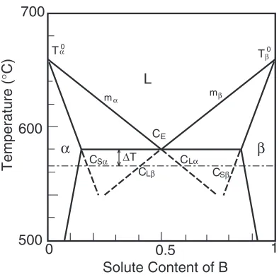
2.1 Assumptions of symmetrical phase diagram For simplicity of calculation, similar to Spettle and Brown,9) a symmetrical phase diagram is assumed, shown in Fig. 1. Along with the parameters shown in Fig. 1, the solute diffusion coefficient,DL ¼3:0109m2/s, and the

Gibbs-Thomson coefficient, ¼2:0107Km, are intro-duced. The symbols and values used in this calculation are listed in Appendix.

2.2 Domain of the calculation

A rectangular shaped domain is used for the cell-automaton calculation, consisting of N cells for the trans-verse direction, where the temperatures are constant, multi-plied byM cells for the longitudinal direction, along which the crystals would grow (see Fig. 2). The periodic boundary condition is employed as the boundary condition concerning the edge of the domain for the growth direction. This means that the sum of the numbers of seeds of the first solid phase () and the second solid phase () should divide Nwith no remainder. If a remainder were to exist, the calculation of the field would necessarily be disturbed and a false unstable *1_{Corresponding author, E-mail: [email protected]}

*2_{Present address: Faculty of Engineering and Resource Science, Akita}

University

growth pattern would be obtained. Therefore N is adjusted according to the number of the seeds. N was about 120 to 150 depending on the number of the seeds.Mwas at 300 in most cases.

2.3 Variable temperature field

A variable temperature field is imposed into the domain. The field has a uniform temperature gradient,G ð>0Þwith the direction ofM. The frame of the temperature field moves at a constant velocity,Vel. So the temperature of any cells in the domain dropsGVelt in one step of the calculation, wheretis the time step of the calculation.

2.4 Rules of the calculation for growth and algorithm Each cell has three types of values: the state of cell, STATE, the content of solute,C; and the fraction of solid,fS.

The variable STATE indicates the state of the phase and can hold one of five values: ‘‘1’’ indicates the liquid phase; ‘‘2’’ the /liquid interface (-liquid mixture); ‘‘3’’ the -liquid interface, ‘‘4’’; and ‘‘5’’.

A process controlled by solute diffusion is assumed. The diffusion process is assumed to act only between the cells accompanying the liquid phase; that is between 1–1, 1–2, 1–3, 2–2, 2–3 and 3–3 couples. Diffusion in the solid is neglected. Fick’s diffusion equation is presumed, and the calculation is performed between the neighboring cells. Interactions between a cell and its neighboring ‘‘north’’ cell, ‘‘south’’ cell, ‘‘east’’ cell and ‘‘west’’ cell are accounted for by employing a finite difference calculation. For diffusion between the liquid cell and solid/liquid interface cell, the diffusion coefficient is modified as

D0_L ¼DLð10:5fSÞ ð1Þ

where fS is the fraction of solid in the solid/liquid cell.

For diffusion between interface cells, the diffusion coefficient is modified as

D0_L¼DLð10:5fS10:5f

2

SÞ ð2Þ

where f_S1is the fraction of solid in the first solid/liquid cell and f2

S it that of the second.

Equilibrium solute partitioning is adopted. In the/liquid interface (STATE 2) or /liquid interface (STATE 3), the fraction of solid is calculated by

fS¼

CCL

CSCL

ð3Þ

whereCis the average content of the solute in the cell,CSthe

solid content and CL the liquid content with the latter two

corresponding to the extension of the liquidus/solidus line of the phase diagram at the imposed temperature. Due to consideration of the Gibbs-Thomson effect, the content CL

is somewhat modified from the quasi-equilibrium diagram for calculation of solute diffusion as

C_Lnew¼TT0

m : ð4Þ

Where T0 is T0 or T

0 andmis m or m. The curvature of the solid/liquid interface is calculated with the box-counting method.10)

Transition of STATE is formulated as follows: if fS

becomes greater than unity, STATE¼2 changes to 4 and STATE¼3 changes to 5; if more than three cells have STATE¼4 in the eight neighboring cells around a cell of STATE¼1, the cell of STATE 1 changes to 2; if more than three cells have STATE¼5 in the eight neighboring cells around a cell of STATE¼1, the cell of STATE¼1changes to 3. The former rule seems reasonable but the latter rules look somewhat artificial. This algorithm is adopted because of the lack of movement of the =boundary in the cell-automaton model and due to the growth rule of Spittle and Brown.9)

2.5 Estimate of the lamellar spacing and the under-cooling

As this study aims to compare the results of the calculation with cell-automaton model with the predictions of the JH model, the lamellar spacing and the undercooling at a given growth velocity ought to be estimated in the calculation. Before estimating the spacing and the undercooling, the growth velocity in the calculation should be estimated. To estimate the growth velocity, parallel lines are drawn atM

100andM50. The timet1is defined in such a way that any STATE½i;M100changes from 1 to 2 or 3, and the timet2 is defined in such a way that any state STATE½i;M50

changes from 1 to 2 or 3. The growth velocity,V, is defined as

V ¼50x=ðt2t1Þ. More precisely, t2t1 is replaced in the calculation as t2t1¼t ðdi f ference o f ste psÞ. In this way, the estimated growth velocity, V, can be compared with the moving speed of the frame of the temperature field, Vel, and it can be determined whether a (quasi) stationary growth is obtained in the calculation. In this study, when 0:995V=Vel1, we have determined that a quasi-stationary growth is achieved.

The spacing, , is calculated near the end stage of the calculation on M50. Actually, when a stable growth is obtained, the spacing does not differ from the spacing which is given by the seeds at the initial step of the calculation. The undercooling, T, is estimated with the temperature of the one forward cell (liquidus) of the/liquid or/liquid cell when any of STATE½i;M30changes from 1 to 2 or 3

α β

0 0.5 1

500 600 700

Temperature (

°

C)

C

CE

Sα CLα

CLβ CSβ

L

Tα0 _T0

β

m_α mβ

∆T

Solute Content of B

(/liquid or/liquid). This method might overestimate the undercooling, but the estimated error is less than 0.005 K (Gx) whenG¼5103_{K/m andx¼10}6_m.

2.6 Procedure of calculation

The temperature gradient,G, was fixed as 5103_K/m. The moving speed of the frame of the temperature field,Vel, was in the range between106_and104_{m/s. The cases for}

Vel¼1106_,2106_,5106_and1105_{m/s, etc.,} were calculated.

The initial seeds were given in the½i;1row as the value of STATE¼2 or 3 (/liquidus or /liqudus). Therefore, the initial lamellar spacing was given asxðns

þnsÞ, where

ns

is the number of seeds of/liquid andns is the number of seeds of /liquid. By changing the number, nsþns, the lamellar spacing of the seeds was adjusted.xwas fixed as 106m for most cases. But as adopting too small a number of seed cells is impractical for the examination of the growth stability (remembering that if more than three neighboring cells are or , the cell changes to /liquid or /liquid), we fixed the smallest number of seed cells at five, and x was changed as an adjustment for the initial lamellar spacing.

The growth structures were displayed in a real time and/or after calculation as accelerated animation. From these observations, stable growth or unstable growth could be determined, and operating ranges of lamellar spacing for stable growth were obtained. The values of spacings and the undercooling were also compared with the JH model. N cells

M

cells

periodic boundary condition

periodic boundary condition

t t

1 2

Fig. 2 Schematic diagram of the domain for calculation.

(a) (b) (c)

Fig. 3 Growth patterns. (a)start¼1:6105m; showing an unstable growth, (b) start¼1:2105m; showing a stable growth,

2.7 JH model

The material parameters for the JH model4)_{were same as}

those used for the cell-automaton calculations listed in Appendix. In addition to these parameters, the contact angles of the liquid/solid interface at the triple-phase junction, , were assumed as 45 degrees for both phases. This meant that the prediction of the JH model could change by a factor of 2, because influences the capillarity terms of the JH model solution through sine function.

The JH model4)_{describes the minimum lamellar spacing,}

, and the growth undercooling of the interface,T, through the growth velocity,V, as

2V ¼ a L

QL ð5Þ

and

T2

V ¼4m

2_aL_QL _ð6Þ

where,m;QL_;aL_{are constants given by}

1

m¼

1

jmj

þ 1

m

ð7Þ

QL¼Pð1þÞ

2_C 0

DL

ð8Þ

aL¼2ð1þÞ a L

jmj

þ a

L

m !

ð9Þ

and;P;aL;aLare

¼ f f

ð10Þ

P¼X

1

n¼1 1

n

3

sin2ðnfÞ ð11Þ

aL¼sin ð12Þ

aL¼sin: ð13Þ

The two analytical equations representing the lamellar spacing and the growth undercooling are based on several physical presumptions, as will be discussed section 3.4.

3. Results and Discussion

3.1 Stable operating range for the lamellar spacing For a given temperature gradient and a moving speed of the frame of the temperature field, a certain operating range for the lamellar spacing has been obtained. Figure 3 shows three cases of the growth pattern with different seed lamellar spacings forG¼5103_{K/m andVel¼110}5_{m/s, up} to the stage before M¼300. (a) is the case with the seed number of 8 and x¼106_{m, i.e., the seed lamellar} spacing, start is1:6105m. (b) is the case with the seed

number of 6 andx¼106_{m, i.e., the seed lamellar spacing} is 1:2105_{m. (c) is the case with the seed number of 7} and x¼5107m, i.e., the seed lamellar spacing is 7:0106m. Because,xof the case (c), is a half of that of (a) or (b), the domain of this case is smaller than that of (a) or (b). Figure 3(a) and (c) show unstable growth patterns. In contrast, Fig. 3(b) shows a stable growth pattern. Beyond M¼300, the calculations with the cases of start¼8:0

106_{m, 1:010}5_{m, and1:210}5_{m have been carried} out up to the stage before M¼700, and the velocities of lamellar coupled growth reached9:9929:998106_m/s. Stable stationary growth has been confirmed for these. Through these calculations, a stable operating range has been obtained for the temperature conditions withG¼5

103K/m and Vel¼1106m/s, 2106m/s, and 5

106m/s, 1105m/s. For the case ofG¼5103K/m and Vel¼2105m/s, there was only one stable seed spacing, and for the cases of Vel¼5105m/s and

Vel¼1104_{m/s with G¼510}3_{K/m, only one} un-stationary stable pattern (that is, stable but with variable growth velocity) was obtained respectively.

3.2 Comparison of the lamellar spacings with the predictions of Jackson-Hunt model

In Fig. 4, the gained lamellar spacings in this cell-automaton calculation are compared with the predictions of the JH model. In the figure, the open circle denotes (quasi) stationary stable growth, and the symbol ‘‘x’’ denotes unstable growth. Note that the lamellar spacing of the latter case is the seed spacing, start, not the spacing at the end

of the calculation,. The open square denotes unstationary stable growth of the cases with Vel¼5105m/s and 1104m/s.

The solid lines illustrates the prediction of the JH model. The results of the cell-automaton method coincide with the JH model within a factor of about two for the cases of stable stationary growth. That is interesting.

3.3 Liquid undercooling at the interface

The liquid undercooling of the forward cell on the top of the interface was estimated in the calculation. Figure 5 shows the results of the cases of stable growth. The prediction of the JH model is also drawn as a straight line. Besides the unstationary growth case (open square), the results calculated agree with the line within a factor of about two. The estimated values of undercooling were larger than 0.05 K and one order greater than the maximum error, 0.005 K.

JH model Stable stationary growth Unstable stationary growth Unstationary growth

10-6 10-5 10-4

Growth Velocity V/ms-1 10-5

5x10-5

5x10-6

Lamellar Spacing

λ/

m

3.4 Average mean curvature of the growth phase In addition to the results of the lamellar spacing and the liquid undercooling at the interface, the value of the average mean curvature of the growth phase was estimated by calculation near the end stage of the cell-automaton simu-lation. Because the curvature value is localized at each interface cell and changes step by step in the calculation, the values for the -phase were estimated through ½N=2þ1;

N=2þn cells and these mean curvatures were averaged. Figure 6 shows the average mean curvature compared with the growth rate. It appears that the curvature increases as the growth rate increases. The value of the symbol on the upper left of Fig. 6 seems to be somewhat higher than expected. This might be due to the sampling procedure used in the calculation. Other than this, the value coincides with ex-pectations because the curvature has an inverse relationship to the lamellar spacing.

3.5 Comparison of the methologies of JH model and this cell-automaton model

Jackson and Hunt model consists of four steps: (1) it solves a periodic boundary diffusion problem of a solute B in the liquid phase and estimates the solutal undercooling ahead of -phase and-phase; (2) it estimates the curvatures of the

-liquid interface and the-liquid interface and calculates the capillary undercoolings; (3) the average undercoolings of or is assumed to be the sum of the solutal and capillary undercoolings, and the solid-liquid interface is presumed to be macroscopically planar, that is,T_{T¼TT, where,TT} is the average undercooling of the-liquid interface andT_T is that of the-liquid interface; (4) finally, that the eutectic structure grows near the extreme condition, that is, the structure grows at the minimum undercooling varying is assumed, and the two equations describing and T are gained.

In this cell automaton method both the diffusion of solute B and the capillary undercooling are taken in account, although they are conducted with a finite diffrence calcuation and a box-counting method. In this method, the assumpions of a macroscopically isothermal interface and the extreme condition are not introduced. Instead, the rule are adopted that the liquid changes to -liquid cell or -liquid cell according to the numbers of the solid cell ( or ) in the neighboring eight cells. Changingstart(the spacing of seeds

and ), stable growth or unstable growth are gained naturally as results of calculations. Operating ranges of the lamellar spacing for a fixed growth condions are gained, which were explained in the JH model as competition between lamellar growth and rod-like growth.

Ultimately, this cell-automaton method does not need the two ad hoc assumptiions, the macroscopically planar inter-face and the extreme condition. Although the ‘‘-liquid or -liquid selection rule’’ is a somewhat artificial, the agreement of the results between the JH model and this model is striking. This suggests the classical value of the Jackson and Hunt model and usefulness of the numerical calculation method for the case where analytical modelling is difficult.

4. Summary

A cell-automaton method was introduced to simulate the growth of eutectic solidification of a binary alloy. Operating ranges for stable, quasi-sationary growth have been obtained corresponding to the moving spped of the frame of temper-ature field and the tempertemper-ature gradient of the field. For stable, quasi-stationary growth, the estimated values of lamellar spacing and the undercooling of the liquid at the solid/liquid interface have agreed with the predictions of Jackson and Hunt model within a factor of two.

REFERENCES

1) C. Zene: Trans. Metall Soc. AIME167(1946) 550. 2) M. Hillert: Jernkontorets Ann.141(1957) 757.

3) W. A. Tiller: Liquid Metals and Solidification, (Am. Soc. Metals, Metals Park, Ohaio, 1958).

4) K. A. Jackson and J. D. Hunt: Trans. Metall Soc. AIME236(1966) 1129.

5) T. Sato and Y. Sayama: J. Cryst. Growth22(1974) 259. 6) D. J. Fisher and W. Kurz: Acta Metall.28(1980) 777. 7) R. Trivediet al.: Acta Metall.35(1987) 971.

8) T. Himemiya and T. Umeda: Mater. Trans. JIM40(1999) 665–674. 9) J. A. Spittle and S. G. R. Brown: Acta Metall. Mater.42(1994) 1811. 10) L. Nastac: Acta Mater.47(1999) 4253.

JH model

10-6 10-5 10-4

Growth Velocity V/ms-1 1

0.1

0.01

Undercooling

∆

T

/K

Fig. 5 Growth rates and undercoolings. The open circle denotes a stable stationary growth, and the square denotes a stable non-stationary growth.

10-6 10-5

Growth Rate (V /ms )-1 10

10

5

4

Curvature (

κ

/ m )

-1

Appendix Meanings and values of symbols.

symbol meaning value unit

C average solute content of a cell — %

CE eutectic solute content 50.0 %

CL liquidus content in the phase diagram — %

Cnew

L liquid composition modified by capillary effect — %

CS solidus content in the phase diagram — %

DL diffusion coefficient of solute in the liquid 3:0109 m2/s

fS fraction of solid in a cell — —

G gradient of the temperature field 5103 _K/m

½i;j cell element of i-th in row and j-th in column — —

k solute partitioning coefficient for/liquid interface 0.3 —

k solute partitioning coefficient for/liquid interface 0.3 —

M number of cells along the temperature gradient direction 300 (default) —

m slope of liquidus of-phase 1:6 K/%

m slope of liquidus of-phase 1.6 K/%

N number of cells perpendicular to the temperature gradient direction 120–150 —

n number of seeds for-phase — —

n number of seeds for-phase — —

STATE state of a cell 1, 2, 3, 4, or 5 —

T temperature of a cell — _C

TE temperature of eutectic point 580 C

T0

melting point of pure-phase 660

_C

T0

melting point of pure-phase 660

_C

V growth velocity of the crystal — m/s

Vel moving speed of the temperature field — m/s

T undercooling — K

t time step for calculation 8105_{(default) s}

x length of a cell square 1106_{(default) m}

curvature of solid/liquid interface — m1