Markups and Firm Level Export Status: Comment

Munich Personal RePEc Archive

Markups and Firm-Level Export Status:

Comment

Deng, Zhongqi and Chen, Yongjun

School of Business, Renmin University of China

12 October 2016

Online at

https://mpra.ub.uni-muenchen.de/74494/

Markups and Firm-Level Export Status: Comment

∗

Zhongqi Deng

School of Business

Renmin University of China

Yongjun Chen

School of Business

Renmin University of China

October 12, 2016

Abstract

This paper reviews a recent paper by De Loecker and Warzynski (AER, 2012), which developed

a method (so-called DLW method) to estimate markups (market powers) using plant-level

pro-duction data. Although DLW aimed to explore the relationship between markups and export

behavior, its core value is the estimation method of firm-level markups. However, this paper finds

that the DLW method still has some errors, one is the disadvantages of supply-side model, the

other is that they used an identical equation to estimate markup.

Key words: Market power; DLW method; Supply-side model; Parameters identification

∗_{Acknowledgment: The paper is supported by the Outstanding Innovative Talents Cultivation Funded Programs}

2015 of Renmin Univertity of China.

1

INTRODUCTION

Market power (or markup) is an old topic in the fields of industrial organization and international

trade; many prestigious economists have researched it, such as Chamberlin (1933), Lerner (1934,

1972), Samuelson (1964), Bresnahan (1989), and Tirole (2015). With the rapid development of

empirical methods, this problem has been studied in more depth (e.g., Berry, Levinsohn, and

Pakes, 1995), but to date, there is still no authoritative method to measure market power (or

markup) and accompanying welfare loss.

A recent paper by De Loecker and Warzynski (AER, 2012), henceforth DLW, develops a

method to estimate markups using plant-level production data. The paper has been cited by a lot

of scholars, because the method (so-called DLW method) is relatively easy to operate. Although

this paper aims to explore the relationship between markups and export behavior, its core value

is the estimation method of firm-level markups. However, we find that the DLW method still has

some errors. Because cannot obtain the primitive data, we just give a theoretical explanation.

2

MEARURING METHODS OF MARKUP

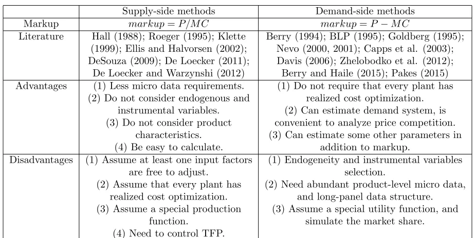
There are two types of models to estimate markup: One is the supply-side model, and the other is

the demand-side model. The former is more convenient (De Loecker and Warzynski, 2012; Berry

and Haile, 2015), but the latter is more popular in academia (for example, Berry, Levinsohn and

Pakes, 1995; Nevo, 2000, 2001). Of course, as shown in Table 1, each method has advantages and

disadvantages. For example, estimation of the demand-side model is relatively difficult, especially

when facing serious endogenous problems1

, but its premise conditions are more tolerant.

Relies on the first order condition (FOC) of cost minimization, DLW gave the expression of

1

Supply-side methods Demand-side methods Markup markup=P/M C markup=P−M C

Literature Hall (1988); Roeger (1995); Klette Berry (1994); BLP (1995); Goldberg (1995); (1999); Ellis and Halvorsen (2002); Nevo (2000, 2001); Capps et al. (2003); DeSouza (2009); De Loecker (2011); Davis (2006); Zhelobodko et al. (2012); De Loecker and Warzynshi (2012) Berry and Haile (2015); Pakes (2015) Advantages (1) Less micro data requirements. (1) Do not require that every plant has

(2) Do not consider endogenous and realized cost optimization. instrumental variables. (2) Can estimate demand system, is (3) Do not consider product convenient to analyze price competition.

characteristics. (3) Can estimate some other parameters in (4) Be easy to calculate. addition to markup.

Disadvantages (1) Assume at least one input factors (1) Endogeneity and instrumental variables are free to adjust. selection.

(2) Assume that every plant has (2) Need abundant product-level micro data, realized cost optimization. and long-panel data structure. (3) Assume a special production (3) Assume a special utility function, and

function. simulate the market share. (4) Need to control TFP.

Note: P defines price,M C defines marginal cost. In order to remain consistent with DLW, this paper uses the division-form markup (P/M C), which can also be derived straightforwardly from Lerner index and has no unit.

Source: Summarized by the authors.

Table 1: Supply-side and demand-side methods of markup estimation

markup as follows:

µit ≡

Pit

M Cit

= (∂QitXit

∂XitQit

)/(P

X itXit

PitQit

) = (∂QitXit

∂XitQit

)/(P

X itXit

Rit

) = θ

X it

αX it

. (2.1)

whereθX

it denotes the output elasticity on inputX,α X

it denotes the share of expenditures on input

X, and P, Q,R denote product price, quantity, and sales revenue, respectively. To be specific,

the DLW method estimates markups as follows:

1. Estimate θX

it and random disturbance term using ACF method

2

;

2. CorrectαX

it using the random disturbance term obtained in the step 1;

3. Calculate markups (µit) using equation (2.1) and steps 1-2.

2

3

PROBLEMS OF DLW METHOD

According to the three steps of DLW method, in order to estimate markups, researchers must first

estimate the output elasticity (θX

it) and expenditure share (α X

it). It is relatively easy to obtain

the data on αX

it, but very difficult to estimateθ X

it. Even DLW used the famous ACF (Ackerberg,

Caves, and Frazer, 2015) method to estimate θX

it, there are still at least two serious problems.

3 .1

Disadvantages of Supply-Side Model

As summarized in Table 1, DLW method belongs to a typical supply-side method. Table 1

men-tioned four disadvantages of supply-side methods: First, this kind of model assumes that at least

one input factor is free to adjust; second, assumes cost-minimizing producer, so factor price is

equal to its value of marginal product (PX

= ∂R/∂X); third, assumes a special

production-function form, for example, translog form, so there may be specification bias3

; fourth, estimating

the output elasticity of a given factor should control the inputs of other factors, productivity level

and the random disturbance term, but productivity and random disturbance term are

unobserv-able, and productivity is endogenous.

If employ ACF method to estimate production function andθX

it, the latter two disadvantages

could be solved partially, but it is still hard to avoid the first two disadvantages. Inputs, in fact,

are difficult to freely adjust, especially DLW chose labour factor, which has adjustment costs

obviously.4

Additionally, factors markets are not necessarily in equilibrium level, so producers

maybe do not realize cost optimization, leading the FOC of cost minimization does not satisfy.

3

If employ a translog or high-degree polynomial production function, the estimate of marginal output (and output elasticity) of a certain factor may be negative, which is caused by the inherent defects of parametric methods. When the estimate of output elasticity (θ) is negative, the DLW method loses efficacy.

4

3 .2

Unobtainable Production Data

According to equation (2.1), DLW gave the estimation formula of markup as µit = θ_itX(αX_it)−1,

whereθX

denotes output elasticity of factorX, i.e.,θX

=∂lnQ/∂lnX (for simplicity in notation,

the subscripts are omitted; the same below). However, in reality, researchers often cannot obtain

the specific data of output (Q), even for producers themselves, because a firm could produce

a variety of products. Generally, researchers can only obtain the data of operating income (or

added value), i.e., R =P Q. Therefore, most researchers use R instead of Q to estimate output

elasticity.5

After usingR instead ofQ, the markup estimated by DLW method is ˆµ= (∂lnR/∂lnX)/αX

,

where∂lnR/∂lnX satisfies

∂R ∂X X R = ∂P ∂X X P + ∂Q ∂X X Q = ∂P ∂Q Q P ∂Q ∂X X Q + ∂Q ∂X X

Q = (1 +

1

η) ∂lnQ

∂lnX. (3.1)

where η denotes price elasticity of demand, ∂lnQ/∂lnX = θX

is the real output elasticity on

input X; becauseQis unobservable, it is also difficult to estimate the real θX

. According to the

relationship between markup and market power, µ= 1/(1−υ), where υ denotes Lerner Index.

And through M R=M C,6

there existsυ=−1/η. Therefore, µ=η/(1 +η), which is equivalent

to 1/µ= 1 + 1/η. Substituting it into equation (3.1), obtain

∂R ∂X X R = 1 µ ∂Q ∂X X

Q. (3.2)

By equation (3.2), using (∂lnR/∂lnX)/αX

to estimate markup in the DLW method is

equiva-lent to ˆµ= (∂lnQ/∂lnX)/(αX

µ), and because the real markup satisfies thatµ= (∂lnQ/∂lnX)/αX

,

5

have ˆµ≡1 theoretically. From the above derivation, if researchers use operating revenue or added

value or similar income indices instead of output quantity to estimate markup, the theoretical

estimate of markup should equal to 1. If the actual estimate results are not equal to 1 (such

as DLW’s results), the main reason is that the premise of cost minimization is not satisfied, i.e.,

∂lnR/∂lnX 6= αX

. Therefore, no matter the estimated markups of DLW method equal to 1 or

not, the results do not reflect the real markups.

According to equation (3.2), the real markup satisfies7

µ= ∂Q

∂X X Q/

∂R ∂X

X

R. (3.3)

But, estimated markup of DLW method is

ˆ

µ= ∂R

∂X X R/α

X

. (3.4)

If actual data satisfies the assumption of DLW method, i.e., cost-minimizing producers, the

equation, ∂lnR/∂lnX = αX

, holds. At this case, from equation (3.4) there exists ˆµ= 1, which

is a paradox8

. As mentioned above, inputs are difficult to freely adjust, and producers are also

hard to make decisions in strict accordance with cost minimization, so in fact factor price is often

lower than its value of marginal product, i.e., ∂R/∂X ≥ PX

, so ∂lnR/∂lnX ≥ αX

. On the

other hand, because the markup of ordinary goods tends to be greater than 1, by equation (3.3)

we know ∂lnQ/∂lnX ≥∂lnR/∂lnX. Therefore, compare equation (3.4) to equation (3.3), both

numerator and denominator are smaller, so DLW overestimating or underestimating markup is

not sure, but obviously the estimation is not correct.

7

From equation (3.3), if use operating income (R) instead of output quantity (Q) to estimate output elasticity of factor (∂lnQ/∂lnX), it is equivalent to assume thatmarkup= 1.

8

According to the assumptions of DLW method, if firms are cost-minimizing producers, then ∂lnR/∂lnX = αX_.

Substitute it into equation (3.3), we can obtain µ = (∂lnQ/∂lnX)/αX_{, which is the calculating formula of markup}

given by DLW. However, becauseQis unobservable, DLW and a lot of other papers that cited the DLW method used

∂lnR/∂lnX to replace ∂lnQ/∂lnX, then ˆµ = (∂lnR/∂lnX)/αX _{= 1 because ∂lnR/∂lnX = α}X_{. Therefore, DLW}

References

Ackerberg, D., K. Caves, and G. Frazer (2015): “Identification Properties of Recent Production Function Estimators,”Econometrica, 83, 2411–2451.

Berry, S.T. (1994): “Estimating Discrete-choice Models of Product Differentiation,” RAND Journal of Economics, 25, 242–262.

Berry, S.T., and P.A. Haile(2015): “Identification in Differentiated Products Markets,”Yale University Working Paper, 21500.

Berry, S.T., J. Levinsohn, and A. Pakes (1995): “Automobile Prices in Market Equilibri-um,” Econometrica, 60, 889–917.

Bresnahan, T. (1989): “Empirical Studies of Industries with Market Power,” in Handbook of Industrial Organization,edited by R. Schamlensee and R. Willing, North-Holland Press.

Capps, C., D. Dranove, and M. Satterthwaite (2003): “Competition and Market Power in Option Demand Markets,”RAND Journal of Economics, 34, 737–763.

Chamberlin, E.H.(1933): The Theory of Monopolistic Competition, Cambridge, MA: Harvard University Press.

Davis, P. (2006): “Spatial Competition in Retail Markets: Movie Theaters,”RAND Journal of Economics, 37, 964–982.

De Loecker, J. (2011): “Product Differentiation Multiproduct Firms, and Estimating the Impact of Trades Liberalization on Productivity,”Econometrica, 79, 1407–1451.

De Loecker, J., and F. Warzynski(2012): “Markups and Firm-level Export Status,” Amer-ican Economic Review, 102, 2437–2471.

DeSouza, S.A. (2009): “Estimating Mark-Ups from Plant-Level Data,” Journal of Industrial Economics, 57, 353–363.

Ellis, G.M., and R. Halvorson (2002): “Estimation of Market Power in a Nonrenewable Resource Industry,”Journal of Political Economy, 110, 883–899.

Goldberg, P.K.(1995): “Product Differentiation and Oligopoly in International Markets: The Case of the U.S. Automobile Industry,”Econometrica, 63, 891–951.

Hall, R.E. (1988): “The Relation between Price and Marginal Cost in U.S. Industry,” Journal of Political Economy, 96, 921–947.

Lerner, A.P. (1972): “The Economics and Politics of Consumer Sovereignty,” American Eco-nomic Review, 62, 258–266.

Nevo, A. (2000): “Mergers with Differentiated Products: The Case of the Ready-to-Eat Cereal Industry,” RAND Journal of Economics, 31, 395–421.

Nevo, A. (2001): “Measuring Market Power in the Ready-to-Eat Cereal Industry,” Economet-rica, 69, 307–342.

Pakes, A. (2015): “Methodological Issues in Analyzing Market Dynamics,” in Advances in Dynamic and Evolutionary Games: Theory, Applications, and Numerical Methods, edited by S. Jorgenson, M. Quincampoix, and T.L. Vincent, Springer Press.

Roeger, A.(1995): “Can Imperfect Competition Explain the Difference between Primal and D-ual Productivity Measures? Estimates for U.S. Manufacturing,”Journal of Political Economy, 103, 316–330.

Samuelson, P.A. (1964): “A. P. Lerner at Sixty,”Review of Economic Studies, 31, 169–178.

Tirole, J.(2015): “Market Failures and Public Policy,”American Economic Review, 105, 1665– 1682.