Modified Effective Specific Heat Method of Solidification Problems
Yau-Chia Liu and Long-Sun Chao
Department of Engineering Science, National Chen Kung University, No. 1, Ta-Hsueh Road, Tainan, 701, Taiwan, R.O.China
In the heat-transfer analysis of a solidification process, the effective specific heat method is conceptually simple to apply while dealing with the latent heat problem. The implementation of computer program is very easy for this method. However, in a time step, if a nodal temperature enters, leaves or jumps over the artificial mushy zone of a pure substance, it cannot calculate the released or absorbed latent heat correctly. If the latent heat is large or the temperature variation is very large, the discontinuity of the effective specific heat will make the iterative convergence difficult to reach. In this work, a modified method is proposed to solve these problems. The method modifies the relation between the temperature and effective specific heat for a solidification process by considering the effect that the temperature at either of two successive time steps is in the mushy zone. The Stefan and Neumann problems with exact solutions were used to test the modified method. The computing results will be compared with those of the effective specific heat method and the enthalpy method. Finally, the feasibility of the modified method is further testified by using a crystal growth problem of GaAs in a Bridgman furnace. [doi:10.2320/matertrans.47.2737]
(Received May 25, 2006; Accepted July 4, 2006; Published November 15, 2006)
Keywords: solidification, Stefan and Neumann problems, modified effective specific heat method, crystal growth
1. Introduction
In a solidification process, the liquid phase at the solid-ification temperature is transformed into the solid one by releasing certain amount of energy, which is the latent heat. The temperature field is directly influenced by the release of the latent heat. Consequently, how to handle the latent heat properly is a key problem in a solidification model.
To simplify the solidification problem, this paper only considers pure substance. Though many mathematical models have been developed to solve solidification problems, they can be divided into two kinds of methods: the front tracking method and the fixed domain method.
1.1 Front tracking method
In this method,1–3) the temperature distributions of solid and liquid phases are solved separately and they are linked by the Stefan condition and the solidification temperature at the solid/liquid interface. At every time step, the location of the interface needs to be traced out, which makes the numerical analysis complicated.
1.2 Fixed domain method
The fixed domain method treats the liquid and solid phases as a computing domain. The temperature fields of both phases are solved together. The following are the common models seen in the literature.
1.2.1 Effective specific heat method
This method puts the latent heat into the specific heat, which is treated as an effective specific heat in the energy equation.3–7)Since the effective specific heat can be regarded as the temperature-dependent property, the implementation of computer program is very easy. The disadvantage of the method is that it predicts the released latent heat less accurate than most other methods.
1.2.2 Enthalpy method
Since enthalpy includes latent heat, it is used and solved in the energy equation instead of temperature.3,6–10)The relation between enthalpy and temperature can be found and it is
treated as a linear one for pure substances. Therefore, the temperature can be calculated according to the relation.
1.2.3 Source term method
The source term method puts the latent heat and liquid fraction together and treats them as a heat source term in the energy equation4,7,11)How to calculate the liquid fraction is the key problem of the method. Voller derived the expression of liquid fraction from the energy equation.11)In solving a solidification problem with this method, the relaxation factor is needed to make the computation having the better convergence.
1.2.4 Temperature recovery method
In the same time step, it is assumed that the total energy change with consideration of latent heat is equal to that without it.12) Without latent heat, the temperature field is solved numerically and then it is corrected by the latent-heat term.
1.2.5 Heat integration method
In this method,6,7) if the temperature of any node drops below the liquidus temperature (or rises above the solidus temperature), the material in the control volume associated with the node is assumed to experience phase change. An accounting for the energy loss by the node at each time step is carried out. The method is computationally economical and can be easily applied to multidimensional problems with isothermal or non-isothermal phase change involved. How-ever, the solution in the region of phase change is inaccurate, as the phase front is not tracked. The accuracy of the results depends on the time step size.
1.2.6 Enthalpy/Specific heat method
The enthalpy/specific heat method3,4,13,14) combines the effective specific heat method with the enthalpy one. It uses the enthalpy to calculate the effective specific heat. The advantage of this method is that it can be directly applied to general heat transfer models. However, when the temper-atures of two successive time steps are the same or very close to each other, the computed value of the effective specific heat is easily divergent in the iterative calculations.
As discussed above, the effective specific heat method is
Special Issue on Advances in Computational Materials Science and Engineering IV
easily applied to solving a solidification problem, especially for a ready-made numerical program of heat transfer. However, its accuracy is not so good and the computation is easily divergent when the Stefan number is small or the temperature field changes suddenly. In this paper, a modified effective specific heat method is proposed to solve these problems. Stefan and Neumann problems with exact solu-tions were used to test the modified method. The computing results will be compared with those of the effective specific heat method and the enthalpy method. Finally, the feasibility of the modified method is further testified by using a crystal growth problem.
2. Problems Description
In this study, the Stefan and Neumann problems with exact solutions15) are used to simulate the solidification process. The mathematical models of these two problems are describ-ed as follows.
2.1 Stefan problem:
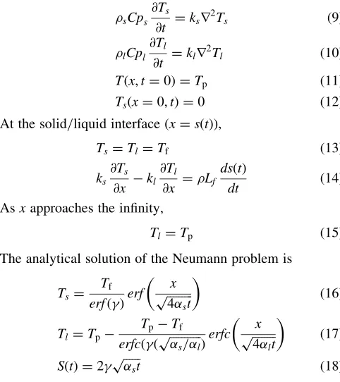
Its physical model covers a one-dimensional semi-infinite region, as shown in Fig. 1. The initial pouring temperature is melting point temperatureTf. Whent0, the temperature at x¼0is equal toTm, which represents the mold temperature. The solidification process proceeds from the left to the right. sðtÞis the position of solid-liquid interface.
In the problem, the basic assumptions are (1) The thermal properties are constant. (2) The effect of natural convection is ignored.
According to the model and assumptions described above, only the temperature field of the solid phased needs to be solved. Its energy equation, initial condition, and boundary conditions can be written as
sCps
@T
@t ¼ksr
2T ð1Þ
Tðx;t¼0Þ ¼Tf ð2Þ
Tsðx¼0;tÞ ¼Tm ð3Þ
At the solid/liquid interface (x¼sðtÞ),
T¼Tf ð4Þ
ks
@Ts
@x ¼Lf dsðtÞ
dt ð5Þ
where Lf is the latent heat. The analytical solution of the problem is
T¼Tmþ
TfTm
erfðÞ erf x
ffiffiffiffiffiffiffiffiffi 4st p
ð6Þ
SðÞ ¼2 ffiffiffiffiffiffist p
ð7Þ
wheresis the thermal diffusivity of solid.is a constant and can be calculated by the following equation
e2erfðÞ ¼ðTfTmÞCps Lf
ffiffiffi
p ð8Þ
2.2 Neumann problem
Its physical model covers a one-dimensional semi-infinite region, which is the same as that of the Stefan problem. The pouring temperatureTp can be larger thanTf and the mold temperatureTmis zero. The basic assumptions are the same as those of the Stefan problem. Hence, the governing equation, initial condition, and boundary condition can be written as
sCps
@Ts
@t ¼ksr 2T
s ð9Þ
lCpl
@Tl
@t ¼klr 2T
l ð10Þ
Tðx;t¼0Þ ¼Tp ð11Þ
Tsðx¼0;tÞ ¼0 ð12Þ
At the solid/liquid interface (x¼sðtÞ),
Ts¼Tl¼Tf ð13Þ
ks
@Ts
@x kl
@Tl
@x ¼Lf dsðtÞ
dt ð14Þ
Asxapproaches the infinity,
Tl¼Tp ð15Þ
The analytical solution of the Neumann problem is
Ts¼ Tf erfðÞerf
x
ffiffiffiffiffiffiffiffiffi 4st p
ð16Þ
Tl¼Tp
TpTf erfcðð ffiffiffiffiffiffiffiffiffiffiffis=l
p
Þerfc x
ffiffiffiffiffiffiffiffi 4lt p
ð17Þ
SðtÞ ¼2 ffiffiffiffiffiffist p
ð18Þ
wherel is the thermal diffusivity of liquid. is a constant and can be calculated by the following equation
expð2Þ
erfðÞ
kl
ks
ffiffiffiffiffi s p
ffiffiffiffi l p
ðTpTfÞexp
2s
l
Tferfcð ffiffiffiffiffiffiffiffiffiffiffis=l p
Þ ¼
Lf
ffiffiffi p
TfCps
ð19Þ
Stefan and Neumann problems are both cover a semi-infinite region. The numerical calculation can be performed only in a finite length region. Accordingly, a computing domain of finite length is applied and the length of the
domain is L. The temperature at x¼L is the pouring
temperature, which is valid as long assðtÞis less thanL.
3. Numerical Method
In this work, the finite difference method was used to solve the temperature field. In the formulation of the difference equation, the centered difference is utilized for the space derivative and the backward difference is for the time derivative. Because the difference equations are nonlinear, the iteration method is adopted to solve these equations. The Solid Liquid
x=0
Tm Tf
x→ ∞
s(t)
[image:2.595.305.546.240.511.2]convergence criterion of the iterative calculations for each time step is defined as
jTknþþ11Tknþ1jmax< " ð20Þ where the superscript n and k are the time index and the iteration number respectively. The subscript max means the maximum value of the temperature differencejTknþþ11Tknþ1j and"is a tolerance."is set to be107for the Stefan problem
and105for the Neumann problem.
In a solidification process, since the release of latent heat will affect the temperature field, a solidification model needs to be applied in the energy equation to deal with its influence. When the temperature reaches solidification temperature, the latent heat will be released in the process of phase change.
In this section, three solidification models will be introduced for solving the Stefan and Neumann problems.
3.1 Effective specific heat method
In this method, the specific heat in the energy equation is replaced by the effective specific heat, which includes the latent heat. The finite-difference formulation of the govern-ing equation can written as
CpeffðTinþ1Þ Tnþ1
i Tin
t ¼k
Tinþþ112Tinþ1þTinþ11
x2 ð21Þ
whereCpeffis the effective specific heat,is density and k is thermal conductivity. The subscript i is the index of space grid.
The relation between the effective specific heat and temperature is shown in Fig. 2. A tiny temperature interval
T taken near the melting point temperature (Tf) will make the shadow area equal to the latent heat. Therefore, the relation between the effective specific heat (Cpeff) and the temperature (T) can be written as
Cpeff ¼
Cpl T >TfþT
1
2
Lf
T þCplþCps
Tf TTTfþT
Cps T <TfT
8 > > < > > :
ð22Þ
where Cpl and Cps are the specific heats of the liquid and solid phases andLf is the latent heat.
Although this method is easy to apply, it still has some disadvantages:
(1) In a time step, if the computed temperature of a node
jumps over the artificial mushy zone, TfT
T TfþT, it will lead to the loss of latent heat. (2) If a nodal temperature enters or leaves the mushy zone
in a time step, the release or absorption of latent heat cannot be calculated correctly.
(3) If the latent heat is large or the large temperature change in a short time and the temperatures of two successive iterations are not both in the mushy zone, the discontinuity of the effective specific heat will make the convergence difficult to reach.
3.2 Enthalpy method
In the enthalpy method, the temperature of the transient term in the energy equation is replaced by enthalpy (e). The energy equation can be rewritten as
@e @t ¼k
@2T
@x2 ð23Þ
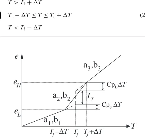
The relation between enthalpy and temperature of a pure substance is shown in Fig. 3. The actual enthalpy curve is discontinuous at the melting temperatureTf, which cannot be used in solving a solidification problem numerically. Con-sequently, two small temperature intervalsTaroundTf are
taken to make an artificial mushy zone. In general, the relation is treated as a linear one,T ¼aþbe, where a and b are constants. In Fig. 3, the constants a and b in the solid, liquid and mushy regions can be written as
a¼a1;b¼b1 e<eL (solid)
a¼a2;b¼b2 eLeeH(mushy) a¼a3;b¼b3 e>eH (liquid)
8 <
: ð24Þ
where
a1¼Tm; b1¼
1
Cps
; eff
Cp
2∆T
f
T
f
T –∆T Tf +∆T
l
Cp
s
Cp
2∆T 2
f l s
L Cp +Cp
+
T
Fig. 2 The relation between the effective specific heat and temperature of a pure substance.
T
e
e
He
La
1,b
1a
3,b
3a
2,b
2L
Cp
∆
T
S
Cp
∆
T
f
L
f
T
–
∆
T
T
fT
f+∆
T
[image:3.595.320.526.76.204.2] [image:3.595.305.540.385.609.2]a2¼TfT
2TCpsðTfTTmÞ CpsTþCplTþLf
;
b2¼ 2T
CpsTþCplTþLf
a3¼Tf Cps
CplðTfTmÞ Lf
Cpl; b3¼
1
Cpl
eL andeH are the enthalpies corresponding toTfT and Tf þT respectively.
The finite difference equation of eq. (23) can be written as
e
nþ1en
t ¼k
Tinþþ112Tinþ1þTinþ11
ðxÞ2 ð25Þ Those temperatures in the right side of the equation above can re-written in terms of enthalpies according to eq. (24).
3.3 Modified effective specific heat method
As mentioned above, in the effective specific heat method,
if a nodal temperature enters, leaves or jumps over the mushy zone in a time step, the release or absorption of latent heat cannot be calculated correctly. For example, in the case
where Tn
i is in the mushy region and T
nþ1
i is in the solid
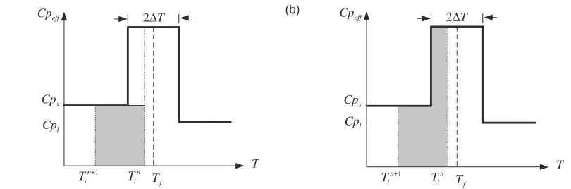
region, as shown in Fig. 4(a), based on eq. (21), the absolute value of energy change in the time step is equal to the shaded area in the figure. However, it is not correct since the latent-heat portion is lost. The correct one is the shades area shown in Fig. 4(b).
For solving the problem of latent heat discussed in the last paragraph, a modified method is proposed in this paper to give a correct calculation of the latent-heat change in a time step. By analyzing the relation between the locations ofTin and Tinþ1 and the mushy zone, there are six cases for a solidification process. With the same analysis of the energy change of Tn
i and T
nþ1
i in Fig. 4, the modified effective
specific heats for these six cases can be written as
Cpeff ¼
Cp1 Tf T>Tnþ1 and TfT >Tn
Cp2 Tf T>Tnþ1 and TfþT TnTfT Cp3 Tf T>Tnþ1 and TfþT <Tn
Cp4 Tf TTnþ1TfþT and TfT TnTfþT
Cp5 Tf TTnþ1TfþT and TfþT <Tn Cp6 Tf þT<Tnþ1 and TfþT <Tn
8 > > > > > > > > < > > > > > > > > :
ð26Þ
where
Cp1¼Cps;
Cp2¼CpsþðCp4CpsÞðT nT
fþTÞ
TnTnþ1 ;
Cp3¼Cpsþ
2TðCp4CpsÞ ðCpsCplÞðTnT
fTÞ
TnTnþ1 ;
Cp4¼1
2
Lf
TþCplþCps
;
Cp5¼Cp4ðCp4CplÞðT
nT
fTÞ
TnTnþ1 ;
Cp6¼Cpl:
In the equations ofCpi’s above, the first term on the right hand side is the non-modified effective specific heat and the second term (if exists) is the modified one.
In the Stefan problem, since the temperature is not bigger thanTf, the artificial mushy zone and eq. (26) must be modified.
The mushy zone changes fromTfT T TfþT toTfT T Tf and the modified one can be expressed as
(a)
n+1 i
T
f
T
eff
Cp
l
Cp
s
Cp
n i
T
T
2∆T (b)
n+1 i
T
f
T
eff
Cp
l
Cp
s
Cp
n i
T
T 2∆T
Fig. 4 The energy change forTn
i in the mushy zone andT nþ1
i in the solid region (a) Effective specific heat method (b) Modified effective
[image:4.595.104.509.74.208.2]Cpeff ¼
Cp1 TfT >Tnþ1 andTfT >Tn Cp7 TfT >Tnþ1 andTf TnTfT
Cp8 TfT Tnþ1Tf andTfTTnTf
8 > < >
: ð27Þ
where
Cp7¼Cpsþ
ðCp8CpsÞðTnT fþTÞ
TnTnþ1 ;
Cp8¼ 1
TðLf þCpsTÞ:
The modified effective specific heat method is easy to use like the effective specific heat method and it calculates the release of latent heat correctly similar to the enthalpy method. Since the modified term is only applied to the case that bothTn
i andT nþ1
i is not in the same region, the modified
effective specific heat can be calculated without any prob-lems.
4. Results and Discussions
The Stefan and Neumann problems, having exact solu-tions, are used to test the modified effective specific heat method, proposed in this work. The computing results are also compared with those of the effective specific heat method and the enthalpy method. For convenience, the dimensionless forms are adopted to discribe the computing results. The dimensionless variables and parameters are shown as follows.
T¼ TTm
TfTm
; t ¼st
L2 ; x
¼x
L;
Ste¼CpsðTfTmÞ Lf
; e ¼ eem CpsðTfTmÞ
where T and e are the dimensionless temperature and
enthalpy. t and x are the dimensionless time and x
coordinate. Ste is the Stefan number. em is the enthalpy
corresponding toTm.
In applying the exact solutions of the Stefan and Neumann problems, firstly the value of should be solved from eq. (8)
or (19). Table 1 indicates the values of for these two
[image:5.595.326.527.289.401.2]problems withSte¼0:1and 1.
Figure 5 shows the computed and exact solutions of the Stefan problem with Ste¼1 att¼3. From this figure, it can be found that the numerical solutions of the effective specific heat, enthalpy and modified effective specific heat methods are close to the exact one. However, the temperature solution of the effective specific heat method deviates a little bit from those of the other methods.
For showing the differences among these three methods clearly, an accumulated error is applied and it is defined as
tolerr¼ X N
i¼1
½ðTiÞexact ðTiÞnumerical2
( )1=2
ð28Þ
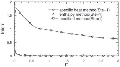
[image:5.595.83.256.435.485.2]where tolerr is the accumulated error and N is the total node number. The subscripts exact and numerical represent the exact and numerical solutions. Figs. 6 and 7 indicate the accumulated error varying with time forSte¼1and 0.1. In these two figures, the accumulated errors of the enthalpy and modified effective specific heat methods are small and very
Table 1 The values of for the Stefan and Neumann problems with
Ste¼0:1, 1.
Ste (Stefan) (Neumann)
0.1 0.22000122 0.21327904
1 0.62006273 0.58274402
0
0 3 5
0.2 0.4 0.6 0.8 1
1 2 4 6 7 8
specific heat method(Ste=1) enthalpy method(Ste=1) modified method(Ste=1) exact sol.(Ste=1)
T*
x*
Fig. 5 The computed and exact solutions of the Stefan Problem forSte¼1 att¼3withx¼0:004,t¼0:005andT¼0:008.
0 0.5 1 1.5 2
0 0.5 1 1.5 2 2.5 3
specific heat method(Ste=1) enthalpy method(Ste=1) modified method(Ste=1)
tolerr
t*
Fig. 6 The accumulated error versus time of the Stefan Problem for
Ste¼1withx¼0:004,t¼0:005andT¼0:008.
0 0.2 0.4 0.6 0.8 1 1.2 1.4 1.6
0 0.5 1 1.5 2 2.5 3
specific heat method(Ste=0.1) enthalpy method(Ste=0.1) modified method(Ste=0.1)
tolerr
t*
Fig. 7 The accumulated error versus time of the Stefan Problem for
[image:5.595.328.527.462.573.2] [image:5.595.324.527.638.758.2] [image:5.595.48.289.745.785.2]close to each other, but the errors of these two methods are significantly smaller than those of the effective specific heat method. From this result, the effective specific heat method has the largest errors since the released latent heat cannot be calculated correctly when a nodal temperature leaves the mushy zone in a time step. The correction of the modified method proposed in this paper can solve this problem.
The computer programs of the numerical simulation were run in a PC with CPU of Intel Celeron 2.26 GHz. Table 2 shows the CPU time of these three methods for the Stefan problem. The effective specific method has the least time and the CPU time of the enthalpy method is almost the same as that of the modified method. The smaller Stefan number has the less CPU time since the smaller Ste has the larger effect of latent heat.
Because the numerical simulation in the Stefan problem does not really include the liquid region, the Neumann problem is used to further test the modified method. SinceTm is equal to zero in the Neumann problem, the temperature
change is very large near x¼0 in the beginning of the
solidification process, which makes the effective specific heat method difficult to obtain convergent solutions. For the
Neumann problem with Ste¼1, only the enthalpy and
modified methods can obtain the convergent solutions, which are shown in Fig. 8. Similar to the Stefan problem, the temperature solutions of these two methods are very close to the exact solution.
Figures 9 and 10 indicate the accumulated error forSte¼
1 and 0.1. The accumulated errors of the enthalpy and
modified effective specific heat methods are also very close to each other. In these two figures, the accumulated errors of Ste¼1 are smaller than those of Ste¼0:1, since the latent-heat effect of the former one is less than that of the latter one.
If the convergent tolerance in eq. (20) rises to 0.015, the temperature solution of the effective specific heat method can be obtained, which is shown in Fig. 11. In this figure, the numerical solution is near to the exact one though the tolerance is not very small. Fig. 12 indicates the accumulated error varying with time for Ste¼1. From Figs. 9 and 12, the accumulated errors of the enthalpy and modified methods are still smaller than those of the effective specific heat method.
Finally, the modified method was applied to solving a thermal flow problem of the crystal growth of GaAs (Gallium
Arsenide) in a Bridgman furnace,16) whose physical model
and coordinate system are shown in Fig. 13.
In the beginning of crystal growth, the furnace wall is heated up to a fixed-linear temperature distribution for a
0 0.2 0.4 0.6 0.8 1 1.2
0 1 2 3 4 5 6 7 8
enthalpy method(Ste=1) modified method(Ste=1) exact sol.(Ste=1)
T*
x*
Fig. 8 The exact solution and the computed ones of the enthalpy and modified method for the Neumann Problem at t¼3 with Ste¼1,
x¼0:004,t¼0:005andT¼0:008.
0 0.1 0.2 0.3 0.4 0.5 0.6 0.7
0 0.5 1 1.5 2 2.5 3
enthalpy method(Ste=1) modified method(Ste=1)
tolerr
t*
Fig. 9 The accumulated errors of the enthalpy and modified methods for the Neumann Problem with Ste¼1, x¼0:004, t¼0:005 and
T¼0:008.
0 0.1 0.2 0.3 0.4 0.5
0 0.5 1 1.5 2 2.5 3
enthalpy method(Ste=0.1) modified method(Ste=0.1)
tolerr
[image:6.595.324.527.71.183.2]t*
Fig. 10 The accumulated errors of the enthalpy and modified methods for the Neumann Problem withSte¼0:1, x¼0:004,t¼0:005 and
T¼0:008.
0 0.2 0.4 0.6 0.8 1 1.2
0 1 2 3 4 5 6 7 8
specific heat method(Ste=1) exact sol.(Ste=1)
T*
x*
Fig. 11 The exact solution and the computed one of the effective specific heat method for the Neumann Problem at t¼3 with Ste¼1,
x¼0:004,t¼0:005andT¼0:008.
Table 2 CPU time of the Stefan Problem for t¼3withx¼0:004,
t¼0:005andT¼0:008.
Specific heat method
Enthalpy method
Modified method
Ste¼10 6 s 8 s 7 s
Ste¼1 3 s 6 s 6 s
[image:6.595.53.286.119.315.2] [image:6.595.327.527.251.363.2] [image:6.595.326.526.430.544.2]certain period of time and then is cooled down to make the crystal grow. The mathematical model is axial-symmetric and the numerical scheme is the finite different method. The
SIMPLEC algorithm17)is used to solve the flow field. The
modified effective specific heat method is utilized to handle the release of latent heat.
Figure 14 shows the numerical solutions of velocity and temperature fields of the GaAs in an ampoule for four time steps withRa¼100. Ra is defined as
Ra¼gTr3o=ðlÞ ð29Þ
where g is the acceleration of gravity, is the volume
coefficient of expansion,rois the outer radius of the ampoule.
Tis the maximum temperature difference of the computing
domain. and l are the kinematic viscosity and thermal
diffusivity of liquid GaAs.
In the figure, it rotates from the vertical to the horizontal for convenience. The direction of gravity is towards the right. Since the cooling rate of the furnace wall is very slow, the temperature distribution of GaAs is similar to that of the furnace wall and most of the isotherms are vertical to the axial direction. The curved isotherm next to the bottom (or the right) of streamlines is the solid/liquid interface. The curved interface is caused by the effects ofks6¼kland latent
heat and it leads to the natural convection, which results in clockwise circulation in the melt. The flow field and curved interface will affect the concentration redistribution of dopant after solidification. Consequently, the precise prediction of the temperature filed is very important to the analysis and the modified specific heat method can help to make it.
5. Conclusion
In this paper, a modified method is proposed to solve the inaccurate and divergent problems of the effective specific method. The Stefan and Neumann problems with exact solutions are used to test the modified method. Finally, the feasibility of the modified method is further testified by using it to solve a crystal growth problem. Based on the results stated above, some conclusions can be made as follow:
(1) The proposed method modifies the relation between the temperature and effective specific heat for a solid-ification process by considering the effect that at either of two successive time steps the temperature is in the artificial mushy zone.
(2) From the computing results of the Stefan and Neumann problems, the modified method can predict the temper-ature distribution as well as the enthalpy method, but more accurately than the effective specific heat method. (3) The effective specific heat method has difficulty to obtain convergent solutions for the Neumann problem, but the enthalpy and modified methods does not. (4) The modified method can be applied as easily as the
effective specific heat method.
(5) The feasibility of the modified is further testified by applying it to solve the solidification process of a crystal growth problem in a Bridgman furnace.
REFERENCES
1) E. M. Sparrow, S. V. Patankar and S. Ramadhyani: J. Heat Transfer99 (1977) 520–531.
2) S. C. Gupta: Comput. Methods Appl. Mech. Eng.189(2000) 525–544. 3) R. W. Lewis and K. Ravindran: Int. J. Numer. Methods Eng.47(2000)
29–59.
4) V. R. Voller and C. R. Swaminathan: Int. J. Numer. Methods Eng.30 (1990) 875–898.
ro ri
Melt
Crystal H
t1
z z
Furnce wall Ampoule
Tfurnace
Tmelting
t2
[image:7.595.326.527.68.215.2]t0 r
Fig. 13 The schematic diagram of a Bridgman Furnace.
L (a)
C g
Time = 0 s, Tmax = 1266°C, Tmin = 1226°C, Ψmax = 0.0005, Ψmin = 0
(b)
CL g
Time = 2560 s, Tmax = 1258°C, Tmin = 1218°C, Ψmax = 0.0005, Ψmin = 0
(c)
CL g
[image:7.595.70.270.73.183.2]Time = 5120 s, Tmax = 1250°C, Tmin = 1210°C, Ψmax = 0.0005, Ψmin = 0
Fig. 14 Solutions of temperature and flow fields with latent heat for
Ra¼100 and ks6¼kl (a) Time¼0s (b) Time¼2560s (c) Time¼
5120s.
0 0.1 0.2 0.3 0.4 0.5 0.6 0.7
0 0.5 1 1.5 2 2.5 3
specific heat method(Ste=1)
tolerr
t*
Fig. 12 The accumulated error of the effective specific heat method for the Neumann Problem withSte¼1,x¼0:004,t¼0:005andT¼
[image:7.595.70.268.257.453.2]5) C. Bonacina and G. Comini: Int. J. Heat Mass Transfer16(1973) 1825– 1832.
6) M. Salcudean and Z. Abdullah: Int. J. Numer. Methods Eng.25(1988) 445–473.
7) Hu Henry and A. A. Stavros: Modelling Simul. Mater. Sci. Eng.4 (1996) 371–396.
8) G. E. Bell and A. S. Wood: Int. J. Numer. Methods Eng.19(1983) 1583–1592.
9) A. W. Date: Int. J. Heat Mass Transfer34(1991) 2231–2283. 10) J. Caldwell and Y. Y. Kwan: Commun. Numer. Meth. Eng.20(2004)
535–545.
11) V. R. Voller and C. R. Swaminathan: Numerical Heat Transfer, Part B.
19(1991) 175–189.
12) T. C. Tszeng, Y. T. Im and S. Kobayashi: Int. J. Mach. Tools Manufact. 29(1989) 107–120.
13) K. Morgan, R. W. Lewis and O. C. Zienkiewicz: Int. J. Num. Methods Eng.13(1978) 1191–1195.
14) J. A. Dantzig: Int. J. Numer. Methods Eng.28(1989) 1769–1785. 15) H. S. Carslaw and J. C. Jaeger:Conduction of Heat in Solids, 2nd ed.,
(Oxford, England 1959) pp. 282–296.
16) J. A. Kafalas and A. H. Bellows: NASA Technical Memorandum.1 (1988) 337–347.