Method for the Determination of Non Chemical Free Energy Contributions as a Function of the Transformed Fraction at Different Stress Levels in Shape Memory Alloys

Method for the Determination of Non-Chemical Free Energy Contributions

as a Function of the Transformed Fraction at Different Stress Levels

in Shape Memory Alloys

Zolta´n Pala´nki

*

_{, Lajos Daro´czi and Dezso L. Beke}

Department of Solid State Physics, University of Debrecen, 4010 Debrecen, P.o.Box 2. Hungary

General equations allowing the determination of the elastic and dissipative energy contributions, as the function of the transformed fraction,, to the martensitic transformation in shape memory alloys are derived. It is shown that the derivatives of these energies bycan be calculated from the measured hysteresis loops. It is illustrated, by the example of our previous experimental results obtained on CuAlNi shape memory alloys at different stress levels,, that our evaluation method gives consistent results with those obtained form the DSC measurements. Furthermore, the- and-dependence of the above derivatives as well as their integral values for (0,1) and (1,0)intervals,i.e.the dissipated energy and the elastic energy stored and released during the forward and reverse transformations, are determined as the function of stress.

(Received February 9, 2005; Accepted March 7, 2005; Published May 15, 2005)

Keywords: shape memory alloy, transformed fraction, elastic and dissipative energy, martensitic transformation

1. Introduction

Determination of the elastic and dissipative energy con-tributions as the function of the transformed fraction, , during martensitic transformations, is a long-standing de-mand for better understanding and tailoring of materials for example for shape memory applications (smart materials). Once determined experimentally they can serve as input parameters for modelling of shape memory or superelastic behaviour. In this paper we describe a new method for the determination of the derivatives of the elastic and dissipative energy terms from the measured hysteresis loops. We show that the integrals of these quantities are in a good accordance with the data obtained from DSC measurements, i.e. our evaluation method is consistent. The method is illustrated on the example of our previous experimental results obtained in CuAlNi shape memory alloys at different stress levels.

2. Equations for the Evaluations

2.1 Derivatives of the free energy contributions

Phase transformations in shape memory alloys (SMA) can take place in both directions (i.e.from the austenite, A, to the martensite, M, and reverse)1) and e.g. for the A!M transformation the change of the Gibbs free energy can be given (if we neglect, as it is usual for SMA, the interface term for nucleation)e.g.as Ref. 2, 3):

G# ¼GMGA¼Gc#þE#þD# ð1Þ Obviously a similar expression can be written for the M!A transformation as well, using the index". Here Gc# is the change in thechemicalGibbs-free energy.E#andD#are the elastic and dissipative energies, respectively. The elastic energy accumulates as well as releases during the processes down and up just because the formation of different variants of the martensite phase is usually accompanied by a development as well as release of an elastic energy field (due to the transformation strain). It is usually supposed that

E¼E# _{¼ E}"_{>0. The dissipative energy is always}

posi-tive in both directions. (In principle, one more additional term, proportional to the entropy production, should be considered, but it can be supposed4–6) _{that this can be} neglected.)

Let us denote the transformed fraction of the martensite phase by(¼1, and ¼0correspond to pure martensite and austenite phases, respectively). The transformation temperature (at which the two phases are in equilibrium for a given) can be given as

@ðG#Þ=@¼gc#þe#ðÞ þd#ðÞ ¼0 ð2Þ where lower cases denote the derivatives of the correspond-ing energy terms. It is assumed thatgc#is independent of and

gc#¼hc#Tsc# ð3Þ withhc# ¼hMhA (<0) and sc#¼sMsA (<0) (the M phase is the low temperature phase). Furthermore, at the ‘‘equilibrium transformation temperature’’, T0 (the temper-ature of zero-change in the chemical free energy);

gc#ðT0Þ ¼0 i.e. T0¼hc#=sc#¼hc"=sc" ð4Þ The temperature at which (2) is equal to zero for¼0as well as ¼1 is the martensite start (Ms) and finish (Mf) temperature, respectively. In general theT#ðÞcurve, defined by (2), gives the lower part of the hysteresis curve (i.e.the

ðT#_{Þcurve). Similarly, theT}"_{ðÞcurve, defined similarly as}

theT#_{ðÞcurve, but for the M!A transformation, gives the}

upper part of the hysteresis curve. Thus

T#ðÞ ¼T0 ½d#ðÞ þe#ðÞ=½sc# and

T"ðÞ ¼T0 ½d"ðÞ þe"ðÞ=½sc# ð5Þ Obviously from theT#_ðÞandT"_{ðÞcurves one can get the}

start and finish temperatures (e.g. for ¼0 Ms¼T0 ½do#þeo#=½sc# and Af ¼T0þ ½do"þeo"=½sc#), which were used in our previous papers7–11) for the determination of the derivatives of dissipative and elastic free energy contributions from experimental data at the start and finish of the martensitic transformation as a function of

*_{Graduate Student, University of Debrecen}

uniaxial stress and/or hydrostatic pressure.

In this paper we will extend this method for the determination of these energies as a function ofat different constant stress levels. Indeed, from (5) one can write

T#ðÞ þT"ðÞ ¼2T0þ ½ðe"ðÞ e#ðÞÞ

þ ðd"ðÞ d#ðÞÞ=½sc# ð6Þ and

T"ðÞ T#ðÞ ¼ ½ðd"ðÞ þd#ðÞÞ

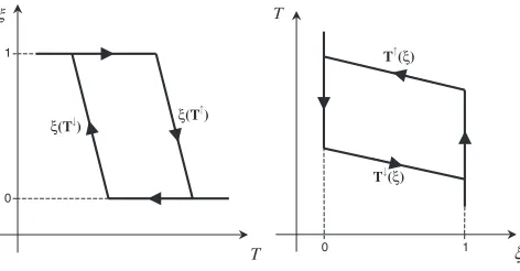
þ ðe"ðÞ þe#ðÞÞ=½sc# ð7Þ Accordingly measuring the T"_{ðÞ andT}#_{ðÞ curves (which}

are the inverse of the#_ðTÞand"_{ðTÞgiving the}

correspond-ing part of the hysteresis curves in theðTÞplots: see Fig. 1 and plotting theT#ðÞ þT"ðÞandT"ðÞ T#ðÞcurves one can get the character of the-dependences of the derivatives of the elastic and dissipative terms. As an approximation we can assume that e#_{ðÞ ¼ e}"_{ðÞ ¼eðÞ (from which the}

assumption E# _{¼ E}"_{¼E mentioned above, follows as}

well) andd"_{ðÞ ¼d}#_{ðÞ ¼dðÞ. Then}

2eðÞ 2sc#T0¼ sc#ðT#ðÞ þT"ðÞÞ ð8Þ and

2dðÞ ¼ sc#ðT"ðÞ T#ðÞÞ ð9Þ It has to be noted that unfortunately we do not know the value ofT0since there is no way for the direct measurement of this quantity. Thus we can determine the elastic energy as the function of the transformed fraction only irrespective of the additive term containingT0.

2.2 Integral quantities

Let us consider the heats of transformation measurablee.g.

in a calorimeter during the forward and reverse transforma-tions. Sincehc#is the latent heat of transformation (per unit fraction), the heat measured for the A)M transformation (cooling down) as well as for the M)A transformation (heating up) are given by

Q#¼

Z1

0

½hc#þe#ðÞ þd#ðÞd ð10Þ

and

Q"¼

Z0

1

½hc"þe"ðÞ þd"ðÞd; ð11Þ

respectively. Now, introducing the following notations:

Z 1

0

hc#d¼

Z0

1

hc"d¼Hcð<0Þ;

Z1

0

d#ðÞd¼D# ð>0Þ;

Z1

0

e#ðÞd¼E# ð>0Þ;

Z0

1

d"ðÞd¼D" ð>0Þ;

Z0

1

e"ðÞd¼E" ð<0Þ;

the relations

Q# ¼HcþE#þD# ð12Þ and

Q" ¼ HcþE"þD" ð13Þ are obtained.

Taking also into account that, according to our assump-tions above,E# ¼ E"¼E(>0) andD#¼D" ¼D(>0):

Q"Q#¼ 2Hc2E ð14Þ

and

Q"_þQ#_{¼2D ð15Þ}

It is important noting that the last equations are strictly valid only if after a cycle the system has come back to the same thermodynamic state,i.e. it does not evolve from cycle to cycle. Furthermore, it can be shown5)_{that (15) is only valid} if the heat capacities of the two phases (cpM andcpA) are equal to each other. If it is not the case then

2D¼Q"þQ#þ ðcpMcpAÞðTATMÞ ð16Þ should be used, whereTAandTMare the corresponding peak temperatures.5)

It can be seen that from the integral of (8) and (9) relations (14) and (15) can be obtained respectively, which —ifsc# is also known from an independent measurement— offer a way for the comparison of the integral of the differential quantities determined from the hysteresis loop and the integrated quantities obtained e.g. from a DSC measure-ments. This can serve as a condition for the self-consistency of our analysis for the determination of thedependence of the dissipative and elastic terms. It is important noting that this condition can be applied even in those cases when

e#ðÞ ¼ e"ðÞ ¼eðÞ(E# ¼ E"¼E) as well asd"ðÞ ¼

d#ðÞ ¼dðÞ(D#¼D"¼D) are not supposed, because the corresponding integrals of (6) and (7) should yield the difference and the sum of (12) and (13), respectively. Thus the above suppositions are necessary only to construct the

dðÞ andeðÞfunctions but the correspondence between the integrals of the derivative quantities (characterized by the

T"_ðÞandT#_{ðÞcurves) and the proper combinations of heats}

measured in a DSC should be valid in general.

2.3 Stress dependence

To determine the stress dependence of the dissipative term

dðÞone has simply measure the dependence of the hysteresis loop on the uniaxial stress, , and from (9) the dð; Þ function can be calculated. On the other hand, for the determination of theeð; Þfunction one has also to take into account that in (8)Tocan be a function ofas well. Since the stress dependent part of gc can be expressed as:"trðÞ

1

0 ξ

T

ξ(T ) ξ(T )

ξ

0 T

1 T (ξ)

T (ξ)

[image:2.595.50.286.72.195.2]

where "trðÞ is the transformation strain and using that @ðgcÞ=@T¼ sc and @ðgcÞ=@¼ "tr, from the Clausius–Clapeyron equation:

@ðgcÞ

@ þ @ðgcÞ

@T dT

d ¼0; ð17Þ

we have

@To

@ ¼ "tr

sc

ð18Þ

where is was also assumed thatsc#andhc#do not depend directly on the temperature and stress. Thus, integrating (18)

T0ðÞ ¼T0ð0Þ

R

0 " tr_ð0_Þd0

sc

ð19Þ

which has to be also used in (8) when the stress dependence of eðÞ term from the T"ð; Þ and T#ð; Þ curves is also determined.

3. Data Analysis

The experimental results, obtained by us in Ref. 11) on wires (1 mm in diameter and 50 mm long) of Cu–24 at%Al– 2.2 at%Ni samples with 0.5 at%B addition, will be used in the analysis described above. For the details of preparation of samples and measurements see Ref. 11), where the temper-ature dependence of the resistance and elongation of samples at different stress levels (up to 10 MPa) were measured. Applying equations (5) at ¼0 as well as ¼1, the derivatives of the elastic and dissipative energy terms were determined as the function of from the transformation temperatures ((As,Af,Ms,Mf)- plots). The transformation entropy was calculated from theRdQ"_=T

A¼ R

dQ#_=T

M¼ sc# relation5)on the basis of the measured DSC curves and sc# ¼ 1:38105J/Km3¼ 1:02J/molK was ob-tained.11)_{It is worth noting that this relation again is valid} only if the heat capacities of the two phases are equal to each other,5)_{but this correction term (ðc}

pMcpAÞlnðTA=TMÞ), is much more negligible as compared to the similar correction in (16). For the sake of simplicity in the following figures sc# ¼scnotation will be used.

In Ref. 11) the "trðÞ was also measured (see Fig. 5 of Ref. 11)) and it was obtained that it can be approximated by a straight line with the slope2:2103MPa1.

Now we extend the analysis made in Ref. 11) and determine the complete dð; Þ as well as eð; Þ functions and the integrals of (8) and (9) will be compared with (14) and (15) calculated from the DSC measurements.

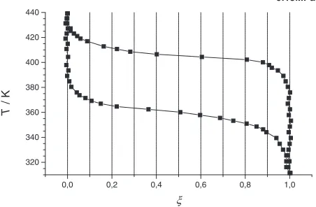
In order to get the necessaryT#_ðÞandT"_{ðÞfunctions first}

the measured hysteresis loops had to be normalized. This was done already in Ref. 11) by removing the transformation independent parts from the original elongation-temperature hysteresis lops and renormalizing their vertical axis to 1. Here we show, as an illustration, a corresponding inverse functionTðÞin Fig. 2.

Thus from the TðÞ functions the T#_{ðÞ andT}"_{ðÞ were}

obtained and, according to (8) and (9), theeðÞ þT0ð0Þscas well as thedðÞfunction were constructed at different stress levels. It is worth noting that while the determination ofT#ðÞ andT"ðÞbetween¼0:1and¼0:9 is easy, the error in reading for!0and!1is higher. Nevertheless, it can

be seen in Figs. 3 and 4 that at the end points (i.e.at¼0and

¼1) the values determined in the usual way fromMs,Mf,

As and Af values obtained in Ref. 11) and denoted by full symbols, usually fit (except one point at¼1for 9.15 MPa) within the error or reading to the values calculated from the normalized hysteresis loops. From such a comparison we recognized that in one case we probably made an error of reading forMfat 2.59 MPa in Ref. 11). Furthermore, in order to get more points on the dissipative energy derivative versus

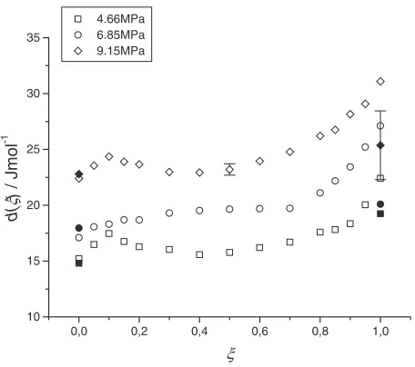
, at small stress level an additional measurement was carried out at¼0:86MPa as well. Thus, we think it is worth to present here the corrected and extended curves corresponding to Figs. 4 and 6 in Ref. 11); see Figs. 5 and 6. The behaviour is similar for the dðÞ curves (only the corrected point for

dð1Þat 2.59 MPa is different, but this value fits better to the overall tendency): both dð0Þ and dð1Þ is approximately constant at low stresses and they show a small increase above 5 MPa. On the other hand the eþT0ð0Þsc versus functions are a bit different: for¼0 this functions shows a decreasing tendency while for ¼1 it is practically constant within the experimental errors.

It can be seen in Figs. 3(a) and 4 that both the eðÞ þ

T0ð0ÞscanddðÞfunctions increase with increasing, and then they change by about 10–40%, respectively between

¼0 and ¼1. It is worth to note that in Fig. 3(a) the

eðÞ þT0ð0Þscvalues have negative sign. From this we can make an estimation for the lower limit ofT0. Since for a given

eð; Þ þT0ð0Þsc has always the lowest value at ¼0 (Fig. 3(a)) and taking also into account Fig. 6 (which shows that theeð0; Þ þT0ð0Þsc function decreases with increas-ing ) we can require that eð0;9:15MPaÞ 0. From this T0ð0Þsc scðT#þT"Þ ¼414J/mol, from which

T0ð0Þ 406K follows. (This condition also corresponds to the well-known relation — see the relations below eq. (5)— ðMsþAfÞ=2¼T0eð0Þ=ðscÞ since for eð0Þ 0,

T0 ðMsþAfÞ=2.) Figure 3(b) shows the e0ðÞ ðeðÞÞ function obtained by takingT0ð0Þsc¼414J/mol. It can be seen that the change in the elastic energy is large and corresponds to a factor of 3–4.

From the integrals of the curves shown in Figs. 3 and 4 the 2Hc2Eas well as2Dquantities, as the function of the stress level, have also been calculated. They are shown in Figs. 7 and 8, respectively as the function of. Here the open

0,0 0,2 0,4 0,6 0,8 1,0

320 340 360 380 400 420 440

9.15MPa

T

/ K

ξ

[image:3.595.314.540.80.228.2]

symbols denote theQ"_Q# _{as well as Q}"_þQ#_{þ ðc}

pM

cpAÞðTATMÞ values calculated from the data (Q";Q#;

TA;TM) obtained from DSC measurements in Ref. 11), while for cpMcpA¼1J/molK was taken in accordance with Ref. 5). It can be seen that both of them increase monotoni-cally with , and the increase in the dissipative energy is small (is about 5%) and detectable only above a certain stress (5 MPa). On the other hand (taking Hc¼ T0ð0ÞSc¼ 414J/mol) an estimate of the relative change of the elastic energy gives about50% in the stress interval investigated. Finally Figs. 9 and 10 show the integral of the elastic and dissipative energies versusrespectively. For calculation of the E0_{ðÞcurve again the T}

0ð0Þ ¼406K value was used as above (i.e. the numerical value can be considered as upper bounds ofE).

In the interpretation of our results it is worth considering that systematic experimental investigations on the stress dependence ofDorEare very rare in the literature and they have not been well understood (for a review of this problem seee.g.Ref. 12, 13)). Furthermore there are no experimental data on the-dependence of the derivatives or integrals of the elastic and dissipative energy terms, and different assump-tions have been used in the simulaassump-tions on the value ofD(in

0,0 0,2 0,4 0,6 0,8 1,0

-420 -410 -400 -390 -380 -370 -360

a

)

4.66MPa

6.85MPa 9.15MPa

e(

ξ

)+

∆

sc T0

(0)

/ Jmol

-1

ξ

0,0 0,2 0,4 0,6 0,8 1,0

-10 0 10 20 30 40 50 60

b

)

4.66MPa

6.85MPa 9.15MPa

e'(

ξ

)

/ Jmol

-1

ξ

Fig. 3 a)eðÞ þT0ð0Þscfunction at different stress levels (full symbols

denote values determined in Ref. 11)). The error bars indicate the error of reading of the corresponding temperatures (0:5K in the middle and

3K at the end points. b)e0_{ðÞfunction obtained withT}

0ð0Þ ¼406K. Since this value is a lower bound forT0,e0ðÞ eðÞholds.

0,0 0,2 0,4 0,6 0,8 1,0

10 15 20 25 30 35

4.66MPa 6.85MPa 9.15MPa

d(

ξ

)

/ Jmol

-1

ξ

Fig. 4 dðÞfunction at different stress levels (full symbols denote values determined in Ref. 11)). The error bars indicate the error estimated similarly as in Fig. 3.

0 2 4 6 8 10

1,2 1,6 2,0 2,4 2,8 3,2 3,6 4,0 4,4

d(ξ=0) d(ξ=1)

d

/ 10

6 Jm

-3

σ / MPa

Fig. 5 Corrected and extended dðÞ curves corresponding to Fig. 4 in Ref. 11).

0 2 4 6 8 10

-58 -57 -56 -55 -54 -53 -52 -51 -50 -49 -48

-47 e(ξ=0)

e(ξ=1)

e+

∆

sc

T0

(0)

/ 10

6 Jm

-3

σ / MPa

Fig. 6 Corrected and extendedeðÞ þT0ð0Þsccurves corresponding to

[image:4.595.54.286.69.460.2] [image:4.595.313.537.74.232.2] [image:4.595.312.539.286.462.2] [image:4.595.56.284.547.749.2]

many cases it was considered to be independent of) or on the-dependence ofdðÞandeðÞderivatives (e.g.in Ref. 14) it was assumed thateðÞis a linear and thusEðÞis a quadratic function of). We believe that our proposal for the analysis of experimentally measured hysteresis loops provide a simple, useful routine for the parallel determination of the above functions in the same sample, and can help to analyze

e.g. the relation between the changes of dissipative and elastic terms (seee.g.Ref. 13)), where only-dependence of

D was evaluated and was rationalized by considering the dissipation of elastic strain energy).

Acknowledgments

The authors are indebted to Professor C. Lexcellent for the critical reading of the manuscript and for the helpful discussions.

This work was supported by the Hungarian grant no. OTKA T 049513.

REFERENCES

1) D. A. Porter and K. E. Easterling:Phase Transformations in Metals and Alloys, (Chapman and Hall, London, 1990) pp. 382–440.

2) H. Funakubo:Shape Memory Alloys, (Gordon and Breach, New York, 1986) pp. 10–14.

3) L. Delaey: Materials Science and Technology, Vol. 5. Phase Tansformations in Materials, ed. by P. Haasen (VHC, 1991) pp. 357– 360.

4) J. Ortin and A. Planes: J. Phys. IV, C4, Suppl. III/1 (1991) 13–23. 5) J. Ortin and A. Planes: Acta Metall.36(1988) 1873–1889. 6) J. Ortin and A. Planes: Acta Metall.37(1989) 1433–1441.

7) L. Daro´czi, D. L. Beke, C. Lexcellent and V. Mertinger: Philos. Mag. B 82(2002) 105–120.

8) L. Daro´czi, D. L. Beke, C. Lexcellent and V. Mertinger: Scr. Mater.43 (2000) 691–697.

9) D. L. Beke, L. Daro´czi, C. Lexcellent and V. Mertinger: J. Phys. IV France11-Pr8 (2001) 119–124.

10) D. L. Beke, L. Daro´czi, C. Lexcellent and V. Mertinger: J. Phys. IV France115(2004) 279–285.

11) L. Daro´czi, Z. Pala´nki, S. Szabo´ and D. L. Beke: Mater. Sci. Eng. A378 (2004) 274–277.

12) H. Sehitoglu, R. Hamilton, H. J. Maier and Y. Chumlyakov: J. Phys. IV France115(2004) 3–10.

13) R. F. Hamilton, H. Sehitoglu, Y. Chumlyakov and H. J. Maier: Acta Mater.52(2004) 3383–3402.

14) B. Peultier, T. Benzineb and E. Patoor: J. Phys. IV France115(2004) 351–359.

0 2 4 6 8 10

680 700 720 740 760 780 800 820 840

-2

∆

Hc

-2E

/ Jmol

-1

σ / MPa

Fig. 7 The integral of the right hand side of eq. (8) at different stress levels (full rectangles). The open symbol is the value obtained from DSC measurements at¼0. It can be seen that the two types of symbols fit very well.

0 2 4 6 8 10

0 10 20 30 40 50 60 70

2D

/ Jmol

-1

σ / MPa

Fig. 8 Integral of the right hand side of eq. (9) at different stress levels (full rectangles). The open rectangle is the value obtained from DSC measure-ments. It can be seen that the two types of symbols fit very well.

0,0 0,2 0,4 0,6 0,8 1,0

0 5 10 15 20 25

9.15MPa

D(

ξ

)

/ Jmol

-1

ξ

Fig. 9 Dissipated energy versus the transformed fraction at 9.15 MPa.

0,0 0,2 0,4 0,6 0,8 1,0

0 5 10 15 20 25

9.15MPa

E'(

ξ

)

/ Jmol

-1

[image:5.595.55.281.70.225.2]

ξ

[image:5.595.313.531.79.239.2] [image:5.595.313.537.290.452.2] [image:5.595.56.283.306.489.2]