Computer Modelling of Manufacturing Processes: The Development of a 2D Axisymmetric Model of the Bridgman Casting Process

Computer Modelling of Manufacturing Processes: The Development of a 2D Axisymmetric Model of the Bridgman Casting Process

S. Battaglioli1, R. P. Mooney1, M. Seredyński3, A. Robinson1, S. McFadden1,2

1. Trinity College Dublin, Dept. of Mechanical & Manufacturing Engineering, Dublin 2, Ireland.

2. Centre for Engineering and Renewable Energy, Magee Campus, Ulster University, Northern Ireland.

3. Warsaw University of Technology, Faculty of Power & Aeronautical Engineering, Poland.

ABSTRACT

Computer modelling is an important tool for investigating manufacturing processes. This paper focuses on a numerical model of the Bridgman solidification casting process, used in applications where the solidification rate and temperature gradient require careful control. A 2D axisymmetric model for transient Bridgman solidification is presented. The governing heat equation is solved using a finite volume method where latent heat evolution is dealt with using the Scheil equation. The model is applied to Bridgman solidification of Al-7wt%Si rods (of varying radii) for different values of Biot number.

KEYWORDS: Bridgman furnace, Solidification, Casting

1.

INTRODUCTION

A validated computer model of a manufacturing process is a valuable tool which aids the engineer in analysing a material as it undergoes the process. Generally, a computer model may be used before, during, or after the process is completed.

A computer model may be used to simulate the process prior to the physical experiment taking place; hence, the engineer will gain insight into the conditions that the material is likely to encounter during the process. Parameters may be varied in the simulations and any predicted changes to the process may be investigated through the simulation results. However, the usefulness of prior simulations is highly dependent on the accuracy of the input data, and verification and validation of the model, Mooney et al. [1].

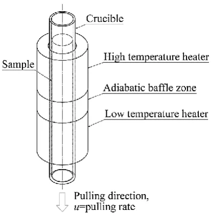
The focus of this study is Bridgman solidification, a process used widely in industry and research. The Bridgman furnace allows the operator to perform directional solidification in a controlled manner. As shown inFig. 1

,

the sample material is held inside a long and slender crucible. Using a series of controlled coaxial heaters and an adiabatic baffle zone, the material is subjected to a thermal gradient, G, along its length, such that the material is fully molten at the hotter end but solid at the colder end. The crucible is translated at a prescribed pulling rate, u, relative to the heaters and in the direction aligned with its axis. Knowing the temperature gradient and the pulling rate, one can estimate the cooling rate of the solidification process (given by product of G and u). The process allows controlled directional solidification.

A novel Bridgman Furnace Front Tracking Model (BFFTM) has been developed by Mooney et al. [4]. This model is based on a Finite Difference Control Volume method and it uses a Front Tracking approach, Browne et al. [5]. The current version of the BFFTM is based on a 1D domain and is valid only for cases where the Biot number (Eq. (6)) is low (Bi < 0.1). A unique feature of BFFTM is that it can model both steady state and transient solidification conditions in the Bridgman furnace. A detailed verification study of the BFFTM is available in literature in Mooney et al. [6].

Fig. 1 Schematic of a Bridgman furnace.

The intended objectives of this paper are:

 to develop a 2D axisymmetric model for transient solidification in a Bridgman furnace based on an enthalpy approach;

 to demonstrate the application of the 2D axisymmetric model where the Biot number is greater than 0.1.

[image:2.477.139.347.306.516.2]

2.

METHODOLOGY

The heat equation to be solved for a 2D axisymmetric solidification problem in a Bridgman furnace is:

𝜕(𝜌𝑐𝑝𝑇)

𝜕𝑡

=

1 𝑟 𝜕 𝜕𝑟

(𝑟𝑘

𝜕𝑇 𝜕𝑟

) +

𝜕 𝜕𝑥

(𝑘

𝜕𝑇 𝜕𝑥

) − 𝑢

𝜕

𝜕𝑥

(𝜌𝑐

𝑝

𝑇) + 𝑢𝜌𝐿

𝜕𝑔_𝑠 𝜕𝑥

+ 𝜌𝐿

𝜕𝑔_𝑠 𝜕𝑡 (1)

where ρ is density; cp, specific heat; T, temperature; t, time; k, thermal

conductivity; u, pulling velocity; L, latent heat; and gs, volumetric solid fraction.

The variable x is the spatial coordinate parallel to the axis and r is the radial coordinate. The term on the left hand side is the change of sensible heat per unit volume. The first and second terms on the right hand side are the conductive rate of heat flow per unit volume in the radial and axial directions. The third and fourth terms on the right hand side are present due to the advection of material at the given pulling velocity. The third term accounts for the advection of sensible heat. The fourth term accounts for the advection of latent heat. Interestingly, the fourth term will only make a contribution to the energy balance in the mushy zone where there is a solid fraction gradient. The last term accounts the release of latent heat due to the solidification process.

2.1 Material

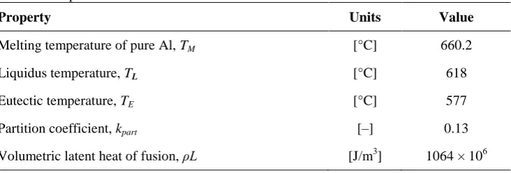
The sample material for the simulation is Al-7wt%Si. The thermophysical properties for the alloy, namely, density, specific heat capacity, and thermal conductivity, were evaluated using polynomial functions of temperature, where the polynomial coefficients were taken from McFadden et al. [7]. Other relevant properties of Al-7wt%Si are shown in Table 1.

The value of solid fraction, gs, during solidification was estimated using the

Scheil equation [8], as follows:

𝑔_𝑠 = 1 − (𝑇𝑀−𝑇

𝑇𝑀−𝑇𝐿) 1

𝑘𝑝𝑎𝑟𝑡−1 ₍₂₎

where kpart is the partition coefficient, and TM and TL are the melting

temperature of pure aluminium and the equilibrium liquidus temperature of Al-7wt%Si, respectively.

[image:3.477.63.429.531.655.2]

Eutectic solidification of the alloy was assumed to be in equilibrium and was treated using a conservative enthalpy method for isothermal freezing at eutectic temperature TE, as described by Voller [9].

Table 1: Properties of Al-7wt%Si

Property Units Value

Melting temperature of pure Al, TM [°C] 660.2

Liquidus temperature, TL [°C] 618

Eutectic temperature, TE [°C] 577

Partition coefficient, kpart [–] 0.13

2.2 Setup & Test Case

The furnace configuration was selected to be equivalent with the Bridgman furnace scenario from Mooney et al. [4]. Fig. 2 shows the high-temperature and low-temperature heaters. An adiabatic baffle zone, with a length of 20 mm,is set

at the centre of the furnace between the heaters. The total length of the computational domain is l=100 mm. Two values of radii were chosen, for the purposes of numerical simulation, rs=8 mm and rs=16 mm.

Since the problem is axisymmetric, an adiabatic boundary condition was assumed at the axis of symmetry and Eq. (1) was solved for half of the sample.

Fig. 2 Bridgman furnace set up.

Dirichlet (first kind) boundary conditions were set at each end of the domain described as follows:

𝑇 = {𝑇_𝑇𝐻 𝑎𝑡 𝑥 = 0, ∀ 𝑟, 𝑡

𝐶 𝑎𝑡 𝑥 = 𝑙, ∀ 𝑟, 𝑡 (3)

The values selected in the simulation were TH=TL+50°C and TC=TE



50°C,

where TL is the equilibrium liquidus temperature of the alloy, and TE is the

equilibrium eutectic temperature.

Robin (third kind) boundary conditions were applied at the sample circumference, i.e., along the heaters in the axial direction. This boundary condition governs the radial heat flow at the circumference and is given as:

−𝑘𝜕𝑇_𝜕𝑟= {_ℎℎ(₍𝑇 − 𝑇_{𝑇 − 𝑇}𝐻) 𝑎𝑡 𝑟 = 𝑟𝑠, 0 < 𝑥 < 𝑥1, ∀ 𝑡 𝐶) 𝑎𝑡 𝑟 = 𝑟𝑠, 𝑥2< 𝑥 < 𝑙 , ∀ 𝑡 (4)

where h is the heat transfer coefficient; its value in the hot and cold zones was set to h=1500 W/(m2K).

Adiabatic boundary condition was set in the baffle, hence:

𝜕𝑇

𝜕𝑟= 0 𝑎𝑡

𝑟 = 𝑟

𝑠

, 𝑥

1

< 𝑥 < 𝑥

2

, ∀ 𝑡

(5)

The Biot number is given as:

𝐵𝑖 =ℎ𝐿𝑐

𝑘 (6)

where Lc is the characteristic length equal to rs/2 (in the case of a

[image:4.477.63.427.177.273.2]

2.3 Numerical Model

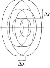
The computational domain was divided in annular control volumes of length ∆x=1 mm and thickness ∆r=1 mm, as shown in Fig. 3. The grid was fixed in space with the sample moving through the domain when u>0.

The heat equation, Eq. (1), was solved using a finite volume numerical model explicit in time. The time step was set equal to ∆t=1×10-3s, which satisfies the stability criterion for the scheme, Jaluria et al. [10].

Since Eq. (2) is a non-linear function of temperature, a Newton-Raphson iterative method, after McFadden et al. [11], was applied to calculate the latent heat term at each time step.

Fig. 3 Annular control volumes.

3.

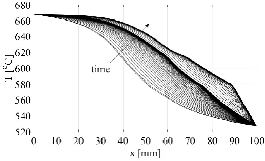
RESULTS

Two different simulations were performed using each radius value. The objective of the first simulation was to obtain a realistic steady temperature profile for the furnace by allowing the temperature to reach equilibrium, when the pulling velocity was set to zero. The initial temperature in the sample was set to

TH and TC in the hot and cold zones, respectively, and a linear distribution of

temperature was applied in the adiabatic zone. The evolution of axial temperature for the first simulation is shown in Fig. 4.

Fig. 5 and Fig. 6 show the steady temperature distribution in the simulated domain (i.e., a section through half of the sample) with rs=8 mm and rs=16 mm,

respectively.

[image:5.477.190.287.184.316.2] [image:5.477.131.358.518.662.2]

Fig. 5 Simulation 1: steady sample temperature distribution for rs=8 mm.

Fig. 6 Simulation 1: steady sample temperature distribution for rs=16 mm.

In the second simulation, the steady solution from the first simulation (i.e., Fig. 4) was set as initial temperature; then the pulling velocity was imposed on the sample by means of two step changes, one at t=100 s with u=0→0.5 mm/s, and one at t=600 s so that u=0.5→1 mm/s. This process is known as velocity jump. Fig. 7shows the resulting evolution in axial temperature.

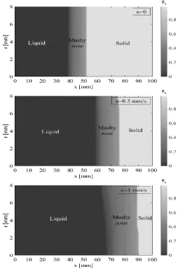
[image:6.477.104.381.56.203.2] [image:6.477.97.382.240.388.2] [image:6.477.115.374.497.654.2]

Fig. 8 Solid fraction distribution at steady state for rs=8 mm.

Fig. 8 shows the distribution of solid fraction, gs, after a steady state is

reached, when the sample is stationary (top plot, u=0 mm/s) and after the two velocity jumps (middle plot, u=0.5 mm/s, and bottom plot, u=1 mm/s) for rs=8

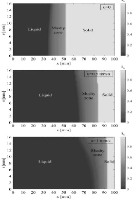
mm. Fig. 10 shows the same data for the simulation where rs=16 mm.

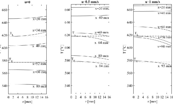
Fig. 9 shows the temperature distribution in the radial direction at fixed axial positions for the three steady states, when rs=16 mm.

4.

DISCUSSION

The results of the first simulation show that realistic temperature profiles were established after the transitory phase.

For both the values of the sample radius, as a consequence of the velocity jumps, the mushy zone moved towards the cold heater zone; at the same time, the width of the mushy zone increased.

It is worthy to note that, when rs=8 mm, the isotherms and lines of constant

[image:7.477.112.367.54.438.2]

radial direction; this demonstrates that, for Bi<0.1, it is acceptabe to assume axial heat flow only.

On the other hand, in Fig. 6, when rs=16 mm (where Bi>0.1) the isotherms

were not flat, rather they were bent in the radial direction, due to the presence of a radial heat flow.

Fig. 9 shows the steady-state temperature profiles (when u=0, 0.5 mm/s, and 1 mm/s), at several axial positions, when rs=16 mm. It is interesting to notice

that for x<40 mm (hot heater region), the temperature at the circumference was higher than the one on the axis, while the opposite situation occurred for x>60

mm (cold heater region), where the temperature at the circumference was lower than the one on the axis. Around the centre of the adiabatic zone the temperature was almost constant in the radial direction. Depending on the axial position of the liquidus and eutectic isotherms, these temperature profiles influenced the shape of the solid and liquid front.

This effect is clearly visible in Fig. 10, where the liquid and solid fronts vary in the radial direction. It may be noted that in the case of u = 0 mm/s, the mushy zone is quite advanced into the higher temperature heater region and this gives the liquid-mush interface a convex shape. When pulling velocity is increased to 0.5 mm/s and 1 mm/s the mushy zone settles deeper into the low-temperature heater region and here the heat flow gives the solid–mush interface a concave shape.

Fig. 9 Steady temperature vs radius at different axial positions, for rs=16 mm.

5.

CONCLUSIONS

A 2D axisymmetric model of the Bridgman process was developed and the results for an Al-7wt%Si alloy were demonstrated.

[image:8.477.74.421.327.539.2]

[image:9.477.107.369.120.513.2]

carried out using a Bridgman furnace. Future works to develop this model include plans to verify the model by comparison with other models and to implement a 2D columnar front tracking algorithm in order to distinguish a columnar region and Columnar to Equiaxed Transition (CET) within the mushy zone.

Fig. 10 Solid fraction distribution at steady state for r=16 mm.

ACKNOWLEDGMENTS

REFERENCES

[1] R. P. Mooney, S. McFadden, “The role of verification in computer modelling: a case study in solidification processing,” proceedings of the 31st International Manufacturing Conference, Cork Institute of Technology, 4-5 Sep 2014, G. Kelly, pp. 173 – 180, 2014.

[2] R. P. Mooney, S. McFadden, Z. Gabalcová, and J. Lapin, “An experimental– numerical method for estimating heat transfer in a Bridgman furnace,” Appl. Therm. Eng., vol. 67, no. 1–2, pp. 61–71, 2014.

[3] R. P. Mooney, U. Hecht, Z. Gabalcová, J. Lapin and S. McFadden, “Directional solidification of a TiAl alloy by combined Bridgman and power-down technique,” Kovové mater., 53, (3), p.187, 2015.

[4] R. P. Mooney, S. McFadden, M. Rebow, and D. J. Browne, “A front tracking model for transient tolidification of Al–7wt%Si in a Bridgman furnace,” T. Indian I. Metals, vol. 65, no. 6, pp. 527–530, 2012.

[5] D. J. Browne, and J. D. Hunt, “A fixed grid front-tracking model of the growth of a columnar front and an equiaxed grain during solidification of an alloy,” Numer. Heat Trans. B, 45, pp. 395–419, 2004.

[6] R. P. Mooney, and S. McFadden, “Order verification of a Bridgman furnace front tracking model in steady state,” Simul. Model. Pract. Th., vol. 48, pp. 24–34, 2014.

[7] S. McFadden, D. J. Browne, and C.-A. Gandin, “A comparison of columnar-to-equiaxed transition prediction methods using simulation of the growing columnar front,” Metall. Mater. Trans. A, vol. 40, no. 3, pp. 662–672, 2009. [8] E. Scheil, “Bemerkungen zur schichtkristallbildung,” Z. Metallkd., vol. 34,

pp. 70–72, 1942.

[9] V. R. Voller, “An overview of numerical methods for solving phase change problems,” Advances in Numerical Heat Transfer, Volume 1, W. J. Minkowycz and E. M. Sparrow, Eds. CRC Press, 1997, pp. 341–380.

[10] Y. Jaluria, and K. E. Torrance, “Computational heat transfer,” Taylor & Francis, New York, 2003.