Special issue on: Coupled Modelling
No. 28 (Vol. 8, No. 4)
December 2003
December 2003
No. 28 (Vol. 8, No. 4)
Special issue on: Coupled Modelling
CLIVAR is an international research programme dealing with climate variability and predictability on time-scales from months to decades.
CLIVAR is a component of the World Climate Research Programme (WCRP). Latest CLIVAR News
•
CLIVAR Conference Reg-istration Deadline for a dis-counted fee is March 15th 2004•
Indian Ocean Panel formed. Visit http://www. clivar.org/organization/ indian/•
Visit the calendar for de-tails of meetings and confer-ences: http://www.clivar. org./calendar/index.htmThis issue has been sponsored by the China Meteorological Administration through the Chinese Academy of Meteorological Sciences.
Exchanges
Exchanges
Coupled Climate Modelling evolves towards comprehensive Earth system modelling encompassing more and more components, such as biosphere, land surface, atmospheric chemistry and carbon cycle.
The PRISM approach described on page 18 will facilitate the exchange of different model components by building up an infrastructure of Earth System Models.
The figure illustrates the complex interactions of the different model components and their increasing demand in computational resources.
The European Network for Earth System Modelling (ENES)
Call for Contributions
We would like to invite the CLIVAR community to submit papers to CLIVAR Exchanges for the next and subsequent issues. The overarching topic of the next issue will be on ‘science related to the South American Low Level Jet Experiment’. The deadline for this issue is January 31, 2004. The topic for the subsequent issue is ‘Applications to CLIVAR Science’ and the deadline is March 31st, 2004.
Guidelines for the submission of papers for CLIVAR Exchanges can be found under: http://www.clivar.org/publications/exchanges/guidel.htm
Atmosphere Models
Ocean Models
Land Surface Models
Terrestrial Biosphere Models
Carbon Cycle and Atmospheric Chemistry The Earth System Unifying the Models
The Predictive Earth System
Megaflops Gigaflops Teraflops Petaflops
Natural Hazard Prediction Hydrology Process
Models Climate / Weather
Models
Evolving Towards Predictive System Models
Wa
ter Cycle
Dear CLIVAR community,
CLIVAR in 2004
5 years after the ‘official’ start of CLIVAR, at the CLIVAR Conference in Paris, the impact of CLIVAR as a major driving force for international coordinated climate research is getting more and more visible. A number of countries already have specific CLIVAR funding lines, others have devoted funding for CLIVAR research under various programmes (e.g. Rapid (UK), DEKLIM (Germany) and others). Even for regions where we expected that the implementation of internationally coordinated research will be difficult, such as Africa or the Southern Ocean, our panels have made considerable progress to develop activities in order to facilitate CLIVAR research.
During the next year our main emphasis will be to assess what we already have accomplished during this first phase of the programme and even more important we will set the course for the future of CLIVAR. The CLIVAR Conference in Baltimore (http://www.clivar2004.org/) will be the milestone for the assessment, supported by a more objective review of the entire programme which will be done during the next months. These two pieces together will document where we stand now, identify gaps, and provide a vision for the future.
New CLIVAR groups developing
In order to address the specific needs for international coordinated projects within the Indian Ocean, CLIVAR has formed an Indian Ocean Panel in collaboration with IOC. The panel will be chaired by Dr. Gary Meyers (CSIRO, Australia) and meets for the first time jointly with the Asian-Australian Monsoon Panel in Pune, India, February 2004. Preliminary information about this group can be accessed through the CLIVAR web site under http://www.clivar.org/organization/indian/. Another group which is currently under development is the CLIVAR Global Synthesis and Observations Panel. This group will address issues related to global observations, data assimilation and synthesis as well as data management.
This issue of Exchanges
Over the years, Exchanges has documented the development and progress of the programme. We started almost 8 years ago reporting mainly from CLIVAR meetings but as more and more science was done under the CLIVAR umbrella, we shifted the scope in that direction. This issue, focusing on coupled modelling, has for the first time a topic that we already had before, 4 years ago. Since a number of meetings related to climate modelling have taken place during this fall, e.g. the International Conference on Earth System Modelling in Hamburg, followed by the second CMIP workshop and
the JSC/CLIVAR Working Group on Coupled Modelling, we thought that it would be very appropriate to focus again on this topic to document the progress made over the past years. Again, as for the previous issues, we have received an overwhelming response. Due to the gracious support of our new sponsors, the Chinese Academy of Sciences, which is now providing funding for the printing of Exchanges, we are able to highlight the wide range of CLIVAR science in the area of coupled modelling. The full suite of contributions, including those of this printed issue, is available in reprint-style pdf-format under: http://www.clivar.org/publications/exchanges/ ex28_cont.html.
Staff news
As some of you might have already heard, my official CLIVAR involvement will end by end of this year. We are very grateful to the German funding agency BMBF who has supported the office and part of my position for more then 8 years. Unfortunately, it was not possible for BMBF to continue their commitment for the ICPO. My new affiliation will be with Peter Lemke, the chairman of the Joint Scientific Committee for WCRP. Although my responsibilities will have a more general WCRP-wide focus, I hope to be able to spend part of my time to support the ICPO and CLIVAR. Nevertheless, I will resign from my function as an editor of Exchanges. Howard Cattle will continue as the lead editor, assisted from staff members, depending on the overarching theme. I would like to thank you all for your contributions and efforts over the past years. It has been a pleasure to work with all of you in the CLIVAR community. I wish you a Happy New Year and all the best for the future.
Andreas Villwock Editorial
As you will have read above, Andreas is moving on from his work for CLIVAR to play a wider WCRP role. During his years with the ICPO, Andreas has been a tower of strength in his provision of support for CLIVAR. Not only has he been the lead editor of Exchanges but he has acted as manager of the CLIVAR web site overall and provided key support, in particular, to CLIVAR’s modelling groups and the CLIVAR/PAGES Intersection. Andreas’s enthusiasm for CLIVAR and his guardianship of it have been boundless and we in the CLIVAR community owe him a debt of gratitude for all of his efforts over the years. We are working out the division of Andreas’s tasks within the ICPO but are indeed grateful to Peter Lemke, Chairman of the JSC, for agreeing that Andreas can spend some of his time on CLIVAR activities. Many thanks, Andreas, and very best wishes in your new job, which is of course still much in the interests of CLIVAR in the wider WCRP context.
A Study of the Antarctic Circumpolar Wave in the NCAR Coupled Model
Janini Pereira1, Ilana Wainer1, Esther Brady2, and
Bette Otto-Bliesner2
1Instituto Oceanográfico da Universidade de São
Paulo, São Paulo, Brazil
2National Center for Atmospheric Research,
Boulder, USA
Corresponding e-mail: [email protected]
Abstract
The simulation results obtained with a version of the National Center for Atmospheric Research/ Community System Model – CSM, run for 150 years, are used to identify the Antarctic Circumpolar Wave. Hovmoeller diagrams show eastward propagating patterns of sea surface temperature and of subsurface ocean temperature anomalies (at 250m depth). In this coupled model ocean dynamics play a predominant role in explaining the Antarctic Circumpolar Wave. Preliminary results from Empirical Orthogonal Function analysis reveal, for example, that the first spatial mode for subsurface temperature exhibits a combination of both zonal wave numbers two and three which is in agreement with other numerical studies that show a predominance of the same wave numbers.
1. Introduction
The Antarctic Circumpolar Wave (ACW) was first discussed by White and Peterson (1996). They used four types of data to characterize it: i) anomalies in sea ice edge (SIE), sea level pressure (SLP), sea surface temperature (SST) and wind stress. The ACW as revealed by their analysis exhibits a wavenumber two structure and takes 8-10 years to travel around the globe. This is also consistent with the ACW observed by Jacobs and Mitchell (1996) using sea level height data.
Analytical ocean-atmosphere coupled models of the ACW were constructed by Qiu and Jin (1997), White et al. (1998) and Haarsma et al. (2000). Qiu and Jin (1997) proposed a mechanism for the ACW based on local ocean-atmosphere interaction. Following this idea, White et al. (1998) using a simplified model, found that in the absence of ocean-atmosphere coupling, the SST anomalies are advected slowly and soon dissipate, whereas with active coupling advection occurs at the observed speed. Haarsma et al. (2000) using the ECBilt model investigated the physical processes and feedback mechanisms of the ACW. In their model, the ACW-like mode is generated by the advective resonance mechanism of Saravanan and McWilliams (1998), which assumes that the ocean passively advects SST anomalies that are generated by the atmospheric circulation anomalies. On the same note, White et al. (2002) found the ACW in the eastern Pacific and western Atlantic sectors to be a result of damped resonance remotely forced by the slow eastward phase propagation of
covarying SST and SLP anomalies associated to what they called Global ENSO Wave (GEW).
In this paper, we investigate the existence of an ACW-like signal in the CSM 1.4 coupled model using 150 years of simulation data. The model description is summarized in section 2. Section 3 contains the preliminary results and discussion. Finally, in section 4 the conclusions are drawn.
2. Model Description
The coupled climate system model contains four components: atmosphere, ocean, land surface processes and sea-ice, as discussed in Bonville and Gent (1998). The atmospheric component, the CCM3, which is described in Kiehl et al. (1998), Hack et al. (1998) and Briegleb and Bromwich (1998), is a spectral model. The standard configuration employs T31 truncation (3,75º) with 18 levels in the vertical. The land surface biophysics model is the LSM 1, described in Bonan (1996), and runs on the same grid as CCM3. The ocean model (NCOM) described in Otto-Bliesner and Brady (2001) has a configuration of 3.6º resolution in longitude and variable resolution in latitude. In the vertical, 25 levels are used, with 3 equal depth levels in the upper 50m and 12 levels in the upper kilometer of the ocean. The sea-ice model is described in Weatherly et al. (1998). The control run used here is also described in Otto-Bliesner and Brady (2001).
3. Results and Discussion
Hovmoeller diagrams of SST anomalies (with the mean seasonal cycle removed) are examined in order to bring out propagation characteristics that could be associated with the ACW mechanism proposed by White and Peterson (1996). The pattern of dominating eastward propagation from the simulation results from year 69 until 77; from year 73 until 81 and from year 76 until 84 is shown in Figure 1 for the latitudinal average between 50ºS – 60ºS. This pattern progresses taking 8 years to circle 360º around the globe. The magnitude of the SST anomalies are as large 0,9ºC in the Pacific sector. Comparison with White and Peterson (1996) shows consistency in magnitude and location with their SST anomalies, obtained from observed data. It is clear that the model is able to capture an ACW-like pattern similar to that observed by White and Peterson (1996).
subsurface temperature anomalies between 225 – 275m in the ECHO-G model, described in Legutke and Voss (1999). They have shown that both salinity and subsurface temperature display eastward propagation characteristics similar to Figure 2. They also discuss two important discernable features; firstly that the magnitude of the anomalies attains a maximum in two regions: the SE Indian Ocean near 90ºE and in the SE Pacific Ocean near 270ºE; and secondly that the propagation rate of the patterns is reduced with depth which does not occur in the CCM-simulated T250 field with respect to the surface.
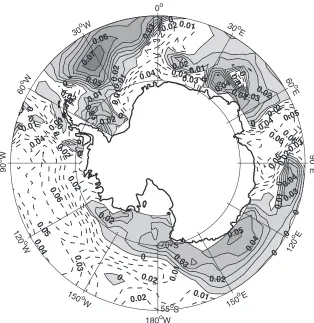
The spatial pattern for the first EOF of T250 anomalies is plotted in Figure 3. It accounts for only 13% of the total variance. This mode shows a combination of both wavenumbers two and three in its spatial pattern that is in part consistent with the ACW in White and Peterson (1996). Other model studies such as that of Christoph et al. (1998), are able to capture an ACW-like oscillation with the same spatial structure. They found propagation characteristics in SST similar to the ACW in the Max Planck Institute coupled general circulation model, though they noted that in this model the ACW-like oscillation had the predominance of both wavenumbers two and three rather than the observed wavenumber two of White and Peterson (1996).
In the CSM 1.4, the subsurface temperature signal that is in phase with the surface hints that it’s ACW-like wave is a result of predominant ocean dynamics rather than air-sea interactions like most other modelling studies: Bonekamp et al. (1999) studied the ACW using experiments with a geostrophic ocean model forced by ECMWF reanalyses. They found that oceanic anomalies with an ACW-like signature could be generated by a one-way atmosphere to ocean forcing. Weisse et al. (1999) forced the same ocean model with spatially realistic and temporally random atmospheric forcing, and generated a variety of ACW-like oceanic anomalies, depending upon the pattern of forcing imposed.
4. Conclusions
[image:4.595.54.321.78.373.2]Variability associated with the ACW-like pattern simulated by the CSM 1.4 bears similarities to the ACW described by White and Peterson (1996). The temporal evolution of the simulated sea-surface temperature anomalies seen in the Hovmoeller diagrams, indicate intermittent eastward propagation with consistent periods of 8 -10 years circling the globe. Considering that the subsurface signal is stronger than the surface, as shown in the EOF analysis, it is thought that air-sea coupling is not essential for generating the structure and the time scale of the ACW-like mode in the CSM. The Fig. 1: Hovmoeller diagrams of SST anomalies (latitudinal average 50ºS
– 60ºS). Unit of temperature in ºC and contour line intervals in 0,2ºC.
[image:4.595.53.322.418.717.2]ACW-like mode shown here could be thought of an oscillation in the interior of the ocean with surface manifestations. Currently more work is being done to understand its genesis in the model and the physical processes associated along with its links to other global scale phenomena, such as ENSO.
Acknowledgements
We thank the following Grants CAPES, CNPQ nº 453523/ 01-3, FAPESP nº 00/2958-7. SGER/ NSF.
References
Bonan, G.B., 1996: A land surface model (LSM version 1.0) for ecological, hydrological, and atmospheric studies: technical description and user’s guide. Technical Note NCAR/TN - 417, 150 pp.
Bonekamp, H., A. Sterl, and G.J. Komen, 1999: Interannual variability in the Southern Ocean from an ocean model forced by European Centre for Medium-Range Weather Forecasts reanalysis fluxes. J. Geophys. Res., 104, 13,317-13,331.
Boville, B., and P.R. Gent, 1998: The NCAR Climate System Model, version one. J. Climate, 11, 1115-1130.
Briegleb, B.P., and D.H. Bromwich, 1998: Polar radiation budgets of the NCAR CCM3. J. Climate, 11, 1246-1269. Christoph, M., T.P. Barnett, and E. Roeckner, 1998: The Antarctic
Circumpolar Wave in a Coupled Ocean-Atmosphere GCM. J. Climate, 11, 1659-1672.
0 0 0 0 0 0 0 0 0 0 0 0 0 0 0 0 0 0 0 0.01 0.01 0.01 0.01 0.02 0.02 0.02 0.02 0.02 0.02 0.03 0.03 0.03 0.0 3 0.03 0.04 0.04 0.04 0.04 0.05 0.05 0.06 0.07 0.060.06 0.06 0.05 0.05 0.05 0.04 0.04 0.04 0.04 0.03 0.03 0.03 0.02 0.02 0.02 0.02 0.02 0.02 0.02 0.02 0.02 0.01 0.01 0.01 0.01 0.01 0.01 0.01 150o W 120 o W 90 o W 60 oW 30 oW 0o 30o E 60 o E 90 o E 120 oE 150 oE
180oW
70oS
[image:5.595.58.372.80.403.2]55oS
Fig. 3: First EOF spacial mode for T250. Contour line intervals in 0,01ºC.
Gent, P.R., F.O. Bryan, G. Danabasoglu, S.C. Doney, W.R. Holland, W.G. Large, and J.C. Mcwilliams, 1998: The NCAR Climate System Model global ocean component. J. Climate, 11, 1287-1306. Haarsma, R.J., F.M. Selten, and J.D. Opsteegh, 2000: On the mechanism of the Antarctic Circumpolar Wave. J. Climate,
13, 1461-1480.
Hack, J.J., J.T. Kiehl, and J. Hurrell, 1998: The hydrologic and thermodynamic characteristics of the NCAR CCM3. J.
Climate, 11, 1179-1206.
Jacobs, G.A., and J.L. Mitchell, 1996: Ocean circulation variations associated with the Antarctic Circumpolar Wave.
Geophys. Res. Lett., 23, 2947-2950.
Kiehl, J.T., J.J. Hack, G. Bonan, B.A. Boville, D. Williamson, and P. Rasch, 1998: The National Center for Atmospheric Research Community Climate Model: CCM3. J. Climate, 11, 1131-1149.
Legutke, S., and R. Voss, 1999: The Hamburg atmosphere-ocean coupled circulation model ECHO-G. Technical Report, No. 18: German Climate Computer Center, Hamburg, Germany. Marsland, S.J., M. Latif, and S. Legutke, 2003: Variability of the Antarctic Circumpolar Wave in a Coupled ocean-Atmosphere Model. Ocean Dynamics, in press.
Otto-Bliesner, B.L., and E.C. Brady, 2001: Tropical Pacific Variability in the NCAR Climate System Model. J. Climate, 14, 3587-3607.
Qiu, B., and F. Jin, 1997: Antarctic circumpolar wave: An indication of ocean-atmosphere coupling in the extratropics. Geophys. Res. Lett., 24, 2585-2588.
Saravanan, R., and J.C. Mcwilliams, 1998: Advective ocean atmosphere interaction: An analytical stochastic model with implications for decadal variability. J. Climate, 11, 165-188.
Weatherly, J., B. Briegleb, W.G. Large, and J. Maslanik, 1998: Sea ice and polar climate in the NCAR CSM. J. Climate,
11, 1472-1486.
Weisse, R., U. Mikolajewicz, A. Sterl, and S.S. Drijfhout, 1999: Stochastically forced Variability in the Antarctic Circumpolar Current. J. Geophys. Res., 104, 11,049-11,064. White, W.B., and R. Peterson, 1996: An Antarctic circumpolar wave in surface pressure, wind, temperature, and sea ice extent. Nature, 380, 699-702.
White, W.B., S.C. Chen, and R. Peterson, 1998: The Antarctic Circumpolar Wave: A beta-effect in ocean-atmosphere coupling over the Southern Ocean. J. Phys. Oceanogr.,
28, 2345-2361.
White, W.B., S.C. Chen, R.J. Allan, and R.C. Stone, 2002: Positive Feedbacks between the Antarctic Circumpolar Wave and the Global El-Niño Southern Oscillation Wave. J.
North Atlantic Decadal Predictability
Mat Collins1, Andrea Carril2, Helge Drange3, Holger
Pohlmann4, Rowan Sutton5 and Laurent Terray6
1 Hadley Centre for Climate Prediction and Research,
Met Office, Exeter, UK.
2 INGV, National Institute of Geophysics and
Volcanology, Bologna, Italy.
3 Nansen Environmental and Remote Sensing Center,
Bergen, Norway.
4 Max-Planck-Institut für Meteorologie,
Hamburg, Germany
5 Centre for Global Atmospheric Modelling,
Department of Meteorology, University of Reading, Reading, UK.
6 CERFACS, Tolouse, France
e-mail: [email protected]
Introduction
There is increasing evidence (from both observations (e.g. Koltermann et al., 1999) and models (e.g. Dong and Sutton, 2001)) of decadal time-scale fluctuations in the circulation of the Atlantic Ocean. Variations in the meridional overturning circulation (MOC) may impact on the surface climate of both the ocean and the atmosphere through changes in the northward transport of heat by the ocean. Predictions of such decadal variations could bring considerable benefit to society, yet these remain unrealised partly because previous studies of predictability have revealed low levels of potential skill (Griffies and Bryan, 1997; Grötzner et al., 1999). This study represents an assessment of the potential predictability of variations in MOC and associated Sea Surface Temperature (SST) anomalies in a range of recent coupled atmosphere-ocean-sea ice models. It is found that, while different models do produce different estimates of predictability, some models show high levels of potential skill on time-scales of decades and longer that may, one day, be exploited by forecasters.
Experimental Design
The coupled model experiments are of the form of “perfect ensemble” experiments, in which ocean initial conditions are fixed and the ensemble is generated by taking different atmospheric initial states. Thus the ensemble spread represents that which would be obtained in a hypothetical operational forecast system in which the ocean state is exactly known and the model is perfect (Collins, 2002). Thus it provides an upper limit on the estimate of predictability. Five models were used to perform experiments (HadCM3 (Gordon et al., 2000), ECHAM5/MPI-OM1 (Latif et al., 2003), ARPEGE3 (Jouzeau et al., 2003), BCM (Furevik et al., 2003) and INGV (Frankignoul et al., 2003)) initiated from unforced control integrations, with ensemble sizes varying from 3 to 9 and the length of the experiments varying from 20-30 years. An attempt was made to initiate experiments
from high, low and (in the case of 2 models) intermediate values of the strength of the MOC. The experiments were performed as part of the European Union Framework 5 project PREDICATE (Sutton et al., 2003) and represent 1340 coupled model years of ensemble experiments, together with 3100 years of control experiments used to assess levels of natural variability. None of the models used employ flux corrections.
Results
The coupled models all have very different magnitudes of natural internal decadal variability in their respective control integrations (Figure 1, page 16). The ECHAM5/ MPI-OM1 model shows the largest variability, with peak-to-peak variations of up to 6 Sverdrups in the MOC and 2K for SSTs averaged in a region of the North Atlantic. The HadCM3 model shows slightly weaker variability than does ECHAM5/MPI-OM1 and the ARPEGE3 and BCM models (which share a common atmosphere) show the weakest. Output from the INGV model is also shown, although it is difficult to assess levels of variability as in this model the ocean component is not in equilibrium resulting in a drift in MOC strength and SST.
Summary
These new model experiments indicate that there may be some potential for initial-value decadal predictions of climate. In general, models that show the highest levels of decadal variability also show the highest levels of decadal predictability: so which model is right? Quantitative validation of the levels of decadal variability in the models is hampered by the short observational record and sparse palaeo-proxy record, and by the fact that these are records of not only the natural internal variability but also forced natural and anthropogenic variations (Collins et al., 2002). Hence it is not possible, at present, to say which model has the more realistic decadal variability and hence more realistic decadal predictability.
Studies of this type, which identify predictable signals, are the first step towards any future operational forecasting system. In any such system the most pressing problem would be in producing an adequate ocean analysis from which to initiate the forecast from sparse subsurface ocean observations. However ocean-only model experiments carried out during the PREDICATE project (Sutton et al., 2003), forced with the same time-history of surface fluxes of heat, moisture and momentum show that this alone may be adequate to constrain the trajectory of the ocean model, at least in terms of the decadal component of the variability of the MOC. Hence a balanced set of fluxes from, e.g., a re-analysis product would be a high priority. Further work should also concentrate on why the models shown here produce such a wide range of decadal variability and predictability.
Acknowledgements
This work was principally supported by the PREDICATE project (EVK2-CT-1999-00020) of the European Union Framework 5 programme, with additional funding from national sources.
References
Collins, M., 2002: Climate Predictability on Interannual to Decadal Time Scales: The Initial Value Problem. Clim.
Dyn., 19, 671-692.
Collins, M., and B. Sinha, 2003: Predictability of decadal variations in the thermohaline circulation and climate.
Geophys. Res. Lett., 30 (6), 10.1029/2002GLO16504.
Collins, M., T.J. Osborn, S.F.B. Tett, K.R. Briffa, and F.H. Schweingruber, 2002: A comparison of the variability of a climate model with palaeo-temperature estimates from a network of tree-ring densities. J. Climate, 15 (13), 1497-1515.
Dong, B., and R.T. Sutton, 2001: The dominant mechanisms of variability in Atlantic ocean heat transport in a coupled ocean-atmosphere GCM. Geophys. Res. Lett., 28, 2445-2448.
Frankignoul, C., E. Kestenare, M. Botzet, A.F. Carril, H. Drange, A. Pardaens, L. Terray, and R. Sutton, 2003: An intercomparison between the surface heat flux feedback in five coupled models, COADS and the NCEP reanalysis. Clim. Dyn., submitted.
Furevik, T., M. Bentsen, H. Drange, I.K.T. Kindem, N.G. Kvamstø, and A. Sorteberg, 2003: Description and validation of the Bergen Climate Model: ARPEGE coupled with MICOM. Clim. Dyn., in press.
Gordon, C., C.A. Senior, H. Banks, J.M. Gregory, T.C. Johns, J.F.B. Mitchell, and R.A. Wood, 2000: The simulation of SST, sea ice extents and ocean heat transport in a version of the Hadley Centre coupled model without flux adjustments. Clim. Dyn., 16, 147-168.
Grötzner, A., M. Latif, A. Timmermann, and R. Voss, 1999: Interannual to decadal predictability in a coupled ocean atmosphere general circulation model. J. Climate, 12, 2607-2624.
Griffies, S.M., and K. Bryan, 1997: Predictability of North Atlantic multidecadal climate variability. Science, 275, 181-184.
Gualdi, S., A. Navarra, E. Guilyardi, and P. Delecluse, 2003: Assessment of the Tropical Indo-Pacific Climate in the SINTEX CGCM. Ann. Geophys., 46 (1), 1-26.
Jouzeau, A., E. Maisonnave, S. Valcke, and L. Terray, 2003: Climatology and Interannual to Decadal Variability diagnosed from a 200-year Global Coupled Experiment. Technical Report TR/CMGC/03/30, CERFACS, Toulouse, France.
Koltermann, K-P., A.V. Sokov, V.P. Tereschenkov, S.A. Dobroliubov, K. Lorbacher, and A. Sy, 1999: Decadal changes in the thermohaline circulation of the North Atlantic. Deep Sea Res. II, 46, 109-138.
Latif, M., E. Roeckner, M. Botzet, M. Esch, H. Haak, S. Hagemann, J. Jungclaus, S. Legutke, S. Marsland, and U. Mikolajewicz, 2003: Reconstructing, monitoring, and predicting multidecadal-scale changes in the North Atlantic thermohaline circulation with sea surface temperature. J. Climate, accepted.
Pohlmann, H., M. Botzet, M. Latif, A., Roesch, M. Wild, and P. Tschuck, 2003: Estimating the long-term predictability potential of a coupled AOGCM. J. Climate, submitted. Sutton, R.T., et al. 2003 PREDICATE final report. See http://
The Response of Climate Variability and Mean State to Climate Change: preliminary results from the CSIRO Mark 3 coupled model
Wenju Cai, Mark Collier, Paul Durack, Hal Gordon, Anthony Hirst, Siobhan O’Farrell and Penny Whetton CSIRO Atmospheric Research
Aspendale, Australia
corresponding e-mail: [email protected]
1. Introduction
The response of the mean state and modes of climate variability to climate change forcings is one of the most important issues in climate research. This issue is particularly relevant for Australia, where a highly variable climate, often characterised by severe floods and drought, is strongly influenced by the El Niño-Southern Oscillation (ENSO), north-south variations in the mid-latitude high-pressure belt position (Pittock, 1973), and, possibly, Indian Ocean sea surface temperature (SST) variations (e.g., Nicholls, 1989). A change in the properties of such modes may result in significant changes to Australian rainfall variability. Further, global warming signals may project onto these modes, contributing to secular trends in rainfall climatology. Trends towards lower rainfall in some regions suggested by global climate models would compound with rising temperatures and potential evaporation to exacerbate the strain on future water resources.
Several of the above aspects have been examined using the CSIRO Mark 2 model, including whether the Pacific warming pattern is El Niño-like or La Niña-like (Cai and Whetton, 2000; 2001) and whether an observed rising trend in mean sea level pressure (MSLP) at southern mid-latitudes (Cai et al., 2003a) can be at least partially attributed to global warming. The Mark 2 model studies are, however, limited by low resolution of the model and the fact that the model ENSO is too weak, with an amplitude of about one third of the observed. Thus the issue of ENSO response to climate change could not be addressed.
A greatly improved, non-flux adjusted, higher-resolution model, referred to as the CSIRO Mark 3 model, has since been established. This model has resolution of 1.85o
longitude, and 1.85o or 0.93o latitude for the atmospheric
and oceanic components, respectively. More details can be found in Gordon et al. (2002). One control and two climate change experiments with the Mark 3 model have been carried out, providing an opportunity to revisit some of the issues discussed above. Here we present some preliminary results. In particular, we focus on processes that potentially control changes in Australian climate variability and rainfall patterns.
2. Model simulations
The two climate change simulations begin in calendar years 1961 and 1871, respectively, and follow the IPCC
A2 emissions scenario for greenhouse gases, sulfate aerosols and ozone concentrations through to 2100. The results from the two climate change simulations are consistent within bounds of natural variability over the 21st century, and the simulations will be referred to as
the “1961 transient” and “1871 transient”, respectively. The 1871 transient simulation has been continued beyond 2100, using perpetual atmospheric concentrations as in 2100. Both experiments include the observed time-varying ozone concentrations (including stratospheric ozone depletion) up to year 2000 and a projection thereafter.
3.Model ENSO Response
A description of ENSO behaviour in the Mark 3 control simulation can be found in Cai et al. (2003b). The SST and wind anomalies associated with ENSO extend somewhat too far into the western Pacific warm pool, in common with many other models. The spectrum of central equatorial SST displays strong power at periods of 3-5 year as observed but also excessive biennial variability (another common model problem). Nevertheless, the otherwise broadly realistic amplitude and pattern of the model ENSO allows us to address how ENSO may respond to climate change.
Spectral analysis of time series of Niño3.4 SST anomalies for the Mark 3 climate change experiment reveals there is little change in the distribution of ENSO frequency during global warming. The anomalies are calculated with reference to a climatology of the control experiment. The model ENSO under a warming climate still has 3-5 year period and biennial components that are as prominent as in the control run (in terms of percentage of the total ENSO variance).
To address the question of change in ENSO amplitude, time series of standard deviation of Niño3.4 SST anomalies (calculated using a 31-year sliding window) for the three Mark 3 experiments and also two experiments using the Mark 2 model, one control and one forced with the IS92A emissions scenario, are plotted in Fig. 1 (page 16). There is little evidence from Fig. 1 of any substantial change in amplitude of ENSO in the climate change simulation. These results suggest that ENSO will continue to be a robust feature of the future climate.
4. Mean State Response
1800 1900 2000 2100 2200 Year
-20 -10 0 10 20
Rainfall (% change)
Observations Control 1871 Transient a)
Qld. Summer
1800 1900 2000 2100 2200
Year -30
-20 -10 0 10
Soil moisture (% change)
Control 1871 transient b)
Qld. Summer
1800 1900 2000 2100 2200
Model Year 25
30 35
Pressure difference (hPa)
Control 1871 Transient Spring SAM
b)
1800 1900 2000 2100 2200
Model Year
25 30 35
Pressure difference (hPa)
Control 1871 Transient Winter SAM
a)
1800 1900 2000 2100 2200
Year 0
1 2
Rainfall (mm day
-1 )
Control 1871 Transient SWWA Winter c)
1800 1900 2000 2100 2200
Year
0 1 2
Rainfall (mm day
-1 )
Control 1871 Transient SWWA Spring
d)
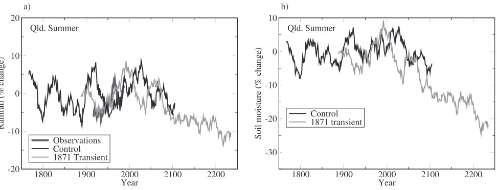
Fig. 3: a) Time series of summer rainfall (11-year running mean) over northeastern Australia (20oS northward and 145oE eastward)
[image:9.595.58.544.81.267.2]in Mark 3 control experiment (dark grey curve), and climate change experiment (light grey curve). b) the same as a) but for soil moisture 10 m below surface.
Fig. 4: Time series of an index (11-point running mean) of the SAM for a) winter season and b) spring season for the control (dark grey curve) and climate change (light grey curve) experiments. The index is defined as the difference between MSLPaveraged over the latitude band 35oS-45oS and that averaged over 55oS-65oS. Also shown are time series of rainfall (mm perday) over
[image:9.595.58.543.336.705.2]First, a time series of the annual mean global surface temperature is constructed. Second, a linear regression is carried out by regressing annual mean SST at each grid point onto the annual mean global surface temperature. Plotted in Fig. 2 are the regression coefficients. Fig. 2 then indicates the warming rate at each grid point per unit increase in global mean temperature. The model El Niño-like pattern is clearly shown with the tongue feature that extends too far into the western Pacific.
Other interesting features include a dipole-like response in the northwest North Atlantic region, strong warming in the Greenland, Iceland and Norwegian Seas, and strong warming in the Tasman Sea region. The warming rate expressed in the western Tasman Sea region is the largest in the Southern Hemisphere, at almost twice the rate of the global mean warming. This prominent feature did not appear as noticeably in the Mark 2 warming experiment, presumably due to the lower resolution (when compared to Mark 3) not resolving the region adequately. The processes controlling this feature are under investigation. The dipole response pattern in the northwest North Atlantic is due to a weakening in North Atlantic Deep Water Formation.
5. Rainfall and Soil Moisture Response in Northeastern Australia
As in Mark 2, a consequence of the model El Niño-like warming pattern is that rainfall over the northeastern Australian region decreases, as shown in Fig. 3a, which shows 11-year running mean rainfall in terms of percentage of the control climatology for the summer season. As warming proceeds, the decreasing trend eventually exceeds the range (-10% to 10%) of decadal and interdecadal variations. The maximum reduction in rainfall reaches 14%. A similar time series of summer soil moisture change for the same region (Fig. 3b) demonstrates a rather more substantial decline in soil moisture, with a maximum reduction reaching 24%. This much larger decrease in the soil moisture is due to increased potential evaporation in a warming climate and illustrates the compounding effect of warming upon a decreasing rainfall trend.
6. Response of the Southern Annular Mode (SAM)
Early studies (e.g., Pittock, 1973) showed that the position of the mid-latitude high-pressure belt fluctuates, so when the high pressure belt moves southwards, MSLP at mid-latitudes increases and rainfall over southwest Western Australia (SWWA) decreases. This is part of the southern annular mode (SAM) (Thompson and Wallace, 2000), the predominant mode of the Southern Hemispheric circulation. Superimposed on these variations is a trend associated with an increasing MSLP in mid-latitudes, and a declining MSLP in high latitudes. This “upward” trend in the SAM indices appeared to form in the late 1960s and early 1970s. In association, since this time, there has been a rainfall decreasing trend in SWWA, with winter rainfall decreasing, in some parts by as much as 20% (Smith et al., 2000; IOCI, 2002). As in Mark 2 warming
experiments (Cai et al., 2003a), the Mark 3 climate change experiments produce an upward trend of the SAM (Fig. 4a and 4b) and a decreasing trend of rainfall over SWWA (Fig. 4c and 4d), in both winter and spring. The rate of the SAM upward trend is slightly greater in the winter season.
In contrast to the observed decrease in winter rainfall, a decrease in the spring season rainfall has yet to be observed in SWWA.
7. Conclusions
Preliminary results from climate change experiments using the CSIRO Mark 3 model, show that ENSO continues to be a robust predominant mode of variability in a warming climate. In each of the two-members of the ensemble forced by the IPCC A2 scenario, there is little change in the ENSO frequency and amplitude. Both ensemble members show an El Nino-like pattern of mean-state change for the tropical Pacific, with a decreasing rainfall trend apparent over northeastern Australia. The impacts of this decreasing rainfall trend are exacerbated by the higher temperature and potential evaporation over the land. Both climate change experiments produce a warming rate in the Tasman Sea region twice as large as that of the global mean surface temperature. As in the CSIRO Mark 2, the southern annual mode index shows an upward trend with increasing MSLP in midlatitudes and a decreasing rainfall trend over SWWA in both the winter and the spring seasons. The relative importance of ozone and greenhouse forcing in generating these changes in each season needs further investigation.
Acknowledgement
We are grateful for the efforts of other members of the Earth System Modelling Programme who are responsible for the development of CSIRO climate models.
References
Cai, W.J., P.H. Whetton, and D.J. Karoly, 2003a: The response of the Antarctic Oscillation to increasing and stabilised atmospheric CO2. J. Climate, 16, 1525-1538.
Cai, W.J., M.A. Collier, H.B. Gordon, and L.J. Waterman, 2003b: Strong ENSO variability and a super-ENSO pair in the CSIRO coupled climate model. Mon. Wea. Rev., 131, 1189-1210.
Cai, W.J., and P.H. Whetton, 2000: Evidence for a time-varying pattern of greenhouse warming in the Pacific Ocean.
Geophys. Res. Lett., 27, 2577-2580.
Cai, W.J., and P.H. Whetton, 2001: A time-varying greenhouse warming pattern and the tropical-extratropical circulation linkage in the Pacific Ocean. J. Climate, 14, 3337-3355.
Gillett, N.P., and D.W.L. Thompson, 2003: Simulation of Recent Southern Hemisphere Climate Change. Science, 302, 273-275.
Gordon, H.B., Rotstayn, L.D., McGregor J.L., Dix M.R., Kowalczyk E.A., O’Farrell S.P., 2002: The CSIRO Mk3 Climate System Model. CSIRO Division of Atmospheric
www.dar.csiro.au/publications/gordon_2002a.pdf. IOCI, 2002: Climate variability and change in the south west
Western Australia. Available from: Indian Ocean Climate Initiative Panel. C/- Department of Environment, Water and Catchment Protection, Hyatt Centre, East Perth, Western Australia 6004, 34 pp. Karoly, D.J., 2003: Ozone and Climate Change. Science, 302,
236-237.
Nicholls, N., 1989: Sea surface temperature and Australian winter rainfall. J. Climate, 2, 965-973.
Pittock, A.B., 1973: Global meridional interactions in stratosphere and troposphere. Quart. J. Roy. Meteor. Soc.,
99, 424-437.
Smith, I.N., P. McIntosh, T.J. Ansell, C.J.C. Reason, and K. McInnes, 2000: Southwest western Australian winter rainfall and its association with Indian Ocean climate variability. Int. J. Climatol., 20, 1913-1930.
Thompson, D.W.L., and J.M. Wallace, 2000: Annular modes in the extratropical circulation. Part I: Month-to-month variability. J. Climate, 13, 1000-1016.
Frank Selten1, Michael Kliphuis1
, and Henk Dijkstra 2 1KNMI, De Bilt, The Netherlands
2Institute for Marine and Atmospheric Research,
Utrecht University, The Netherlands Corresponding e-mail: [email protected]
Introduction
Over the last decade, climate models have grown in complexity at a fast pace. One reason is the inclusion of an increasing number of physical processes that are thought to be relevant. Another reason is the extended range of spatial scales that is captured due to an increased numerical resolution. Both factors increase the computational load of climate model simulations and limit the amount of sensitivity studies that can be performed.
It is an empirical fact that climate models need to be tuned; when components are coupled from realistic initial states, the coupled system drifts toward its own statistical equilibrium. Additional integrations allow researchers to pinpoint possible causes of the drift and adjust specific model parameters to improve the match with the observed behaviour of the climate system. Although improved physical parameterizations and increased resolution should in principle lead to more realistic simulations, it is often only after the ‘tuning’ process that the latest model version generally outperforms the previous.
To assess changes in the climate due to presumed increasing levels of greenhouse gases (GHG) in the near future, often just one or a few transient coupled climate simulations are performed for a given scenario of the future emissions due to the high computational demand of a single simulation. This allows an assessment of the mean climate change. But if one wants to investigate possible changes in the probability and character of extreme events, a large ensemble of such simulations is necessary.
The ensemble experiment
In order to study the probability of extreme events in a changing climate, the Netherlands Centre for Climate
Transient coupled ensemble climate simulations to study changes in the probability of extreme events
Research (CKO) decided to produce a large ensemble of transient climate simulations. This summer the NCAR Community Climate System Model, version 1.4, was ported to the SGI 3800 machine of the Academic Computing Centre at Amsterdam (SARA). During three months, 256 of its processors were dedicated to this project. The choice for CCSM1.4 was motivated by computational constraints, the fact that this version was carefully tuned to simulate the ENSO phenomenon rather well (Otto-Bliesner and Brady, 2002) and the relative little effort involved in preparing the system to suit our purpose.
The system was integrated 62 times for the period 1940-2080. During the historical part of the simulation, GHG concentrations, sulphate aerosols, solar radiation and vulcanic aerosols were prescribed according to observational estimates, kindly provided by C. Ammann (Ammann et al, 2003). From 2000 onwards, the solar constant was held constant and sulphate aerosols were kept fixed. Only the GHG concentrations varied according to a Business-as-Usual scenario. This scenario is similar to the SRES A1 scenario (Dai et al, 2000). The ensemble members differ only in a small random perturbation in the initial temperature field of the atmosphere, enough to lead to entirely different atmospheric evolutions within the first couple of weeks of the integrations. The initial state was obtained from the simulations of Ammann (personal communication).
Some preliminary results
side of the range (1.4 to 5.8 degrees) established in the IPCC Third Assessment Report (2001). This range is based on results from different model simulations and emission scenarios.
For a grid box, partially overlapping the Netherlands, we calculated the mean winter and summer temperatures in all simulations (Fig. 2, grey crosses) and compared these with temperatures from weather station De Bilt in the Netherlands (black dots). Apart from a summer bias of -1.7 degrees Celcius and winter bias of +2.6 degrees Celsius, the range of simulated temperatures covers the observations very well. The hottest summer on record (1947) is also a rare event in the simulations, as is the coldest winter (1963). The probability of extreme hot summers increases faster as might be expected on the basis of the mean warming. In contrast, probabilities of extreme cold winters decrease faster. Extreme cold winters, although more rare, still occur.
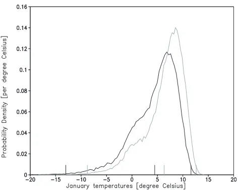
These results suggest that the probability density function (PDF) of temperature not simply shifts with the mean, but changes its shape in the warming climate. Figure 3 shows the PDF for January daily mean temperatures for the same grid point.
Clearly the cold tail depopulates. The one in 10 year cold event warms 4.2 degree Celsius, more than twice as much as the mean warming. Physical causes for the PDF shape changes are currently under study.
We have also looked at the simulation of the North-Atlantic Oscillation based on the simulated mean sea level pressure fields. The simulated NAO pattern compares well with the observed (not shown). Simulation #13 tracks the observed tr end towards
positive NAO index in the past 30 years remarkably well (Fig. 4). However, other members simulate opposite trends; the ensemble mean shows no trend (black line), also not in this century. These preliminary results suggest that the observed trend can be explained by natural, unpredictable, climate fluctuations. Although the ensemble mean NAO index does not change, the ensemble mean global temperature rises. This suggests that the global warming of the past 30 years is not due solely to the trend in the NAO, as suggested in the literature (Hurrell, 1996).
Acknowledgements
[image:12.595.306.539.75.470.2]We wish to thank Bette Otto-Bliesner, Caspar Ammann and Grant Branstator of NCAR for their input to the project. Use of the computing facilities was sponsored Fig. 1: Global mean temperatures of all 62 simulations (light
crosses), the ensemble mean (solid line) and observed temperatures from the Climate Research Unit (dark dots). The CRU timeseries obtained were anomalies wrt the 1960-1990 period. We added the ensemble mean simulated temperature over this period.
[image:12.595.54.283.78.260.2]Fig. 3: Probability density function of daily mean temperatures in the same grid box as Fig. 2, for January for the period 1951-1980 (black solid) and 2051-2080 (grey solid). Short vertical lines indicate the temperatures of the one in 10 year cold extremes (left ones), the mean temperatures (middle ones) and the one in 10 year warm extremes (right ones).
by the National Computing Facilities Foundation (NCF) with financial support from NWO.
Challenge website: http://www.knmi.nl/onderzk/ CKO/Challenge_live
References
Ammann, C.M., J.T. Kiehl, C.S. Zender, B.L. Otto-Bliesner, and R.S. Bradley, 2003: Coupled Simulations of the Twentieth Century including External Forcing. J. Climate, submitted.
Fig. 4: The NAO index based on NCEP-NCAR reanalysis of mean sea-level pressure (dark dots), the NAO index of simulation #13 (light crosses) and the ensemble mean NAO (solid line). Timeseries are low-pass filtered with an 11 year running mean.
Dai, A., T.M.L. Wigley, B.A. Boville, J.T. Kiehl, and L.E. Buja, 2001: Climates of the Twentieth and Twenty-First Centuries Simulated by the NCAR Climate System Model. J. Climate, 14 (4), 485-519.
Hurrell, J.W., 1996: Influence of variations in extratropical wintertime teleconnections on Northern Hemiphere temperature. Geophys. Res. Lett., 23, 665-668.
Otto-Bliesner, B.L., and E.C. Brady, 2001: Tropical Pacific Variability in the NCAR Climate System Model. J.
Climate, 14 (17), 3587-3607.
This Workshop is organized under the auspices of the International CLIVAR Project by the Atlantic Implementation Panel, the Working Group on Ocean Model Development, and the Special Research Programme on the “Dynamics of Thermohaline Circulation Variability” (SFB 460) at Kiel University.
The Workshop intends to bring together expertise from physical oceanographers, geochemists, and ocean and climate modelers, to discuss recent advances and outstanding problems in our understanding of the mechanisms of deep water formation in the subpolar North Atlantic, their relation to large-scale thermohaline circulation (THC) variability and impact on the uptake anthropogenic trace gases, and the future of the THC under changing climate conditions.
Main Goals:
1) To take stock of our understanding and best estimates of the present and future state of the Atlantic Thermohaline Circulation.
2) To guide implementation plans by assessing the capabilities and future needs of THC observing and synthesis systems to detect low-frequency changes or trends.
For further information contact:
Lothar Stramma and Sigrun Komander, IfM Kiel (e-mail: [email protected])
For general information:
http://www.ifm.uni-kiel.de/allgemein/naw2004.htm
Announcement:
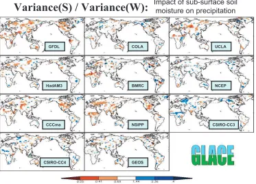
[image:13.595.52.288.208.396.2]GLACE: Quantifying Land-Atmosphere Coupling Strength Across a Broad Range of Climate Models
Randal Koster1, Zhichang Guo2, and Paul Dirmeyer2 1NASA/Goddard Space Flight Center,
Greenbelt, USA
2Center for Ocean-Land-Atmosphere Studies,
Calverton, USA
corresponding e-mail: [email protected]
In analogy to ocean heat content, land surface soil moisture and snow cover have a longer memory than atmospheric quantities and can potentially contribute to atmospheric variability and seasonal predictability. The degree, however, to which the atmosphere responds to land surface anomalies (i.e., the land-atmosphere coupling strength) is still largely unknown. Modeling studies do abound; many AGCMs have quantified, for example, the impact of soil moisture variations on model precipitation. Nevertheless, all such results are keyed to the model’s intrinsic land-atmosphere coupling strength, a model-dependent quantity that is not well determined, validated, or even understood. This coupling strength is not specified explicitly by the modeler but is rather a complex function of the numerous interacting model parameterizations controlling the land surface energy balance, the development of the boundary layer, precipitation generation (particularly convection), and other AGCM features. Most modelers appear to accept their own model’s coupling strength completely on faith, not addressing either its realism or how it compares with that in other models.
The quantification and documentation of coupling strength across a broad range of models would be valuable, if only to serve as a frame of reference when interpreting the experimental results of any particular model. This quantification and documentation is the goal of GLACE (Global Land Atmosphere Coupling Experiment), an experiment jointly sponsored by the CLIVAR Working Group on Seasonal-to-Interannual Prediction (WGSIP) and the GEWEX Global Land Atmosphere System Study (GLASS) panel. In essence, GLACE is a highly controlled AGCM experiment that allows the computation of objective indices of coupling strength – indices that can be directly compared between models. At present, ten AGCM groups have completed the GLACE experiments. Output from a few additional groups is expected soon.
The design of the GLACE experiment follows closely that used by four participants in a recent pilot study (Koster et al., 2002), a study hinting at a wide range of coupling strengths among today’s models. In GLACE, each participating AGCM group generates the following three ensembles of simulations:
•
Ensemble W: Sixteen 92-day simulations spanning June 1 – August 31, using prescribed SSTs from a particular year of interest.•
Ensemble R: Sixteen simulations spanning the same time period and using the same SSTs, but with the following twist: all simulations are forced to maintain the same geographically-varying time series of land surface prognostic variables (soil moistures, surface and subsurface temperatures, etc.). This is achieved by replacing, at every time step, the prognostic variables’ values with those produced at that time step by a particular member of Ensemble W.•
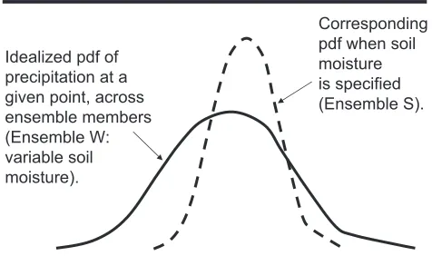
Ensemble S: The same as Ensemble R, except only the subsurface soil moisture prognostic variables are forced to be identical amongst the member simulations. In Ensemble R, the atmospheres in all member simulations see the same time-varying, spatially varying anomalies of temperature and moisture at the land surface. In Ensemble S, they see the same time-varying, spatially varying anomalies of subsurface moisture. In either ensemble, we can quantify coupling strength by examining the agreement in the weather generated amongst the ensemble members (see below). Note that Ensemble S is probably the most relevant to CLIVAR. Subsurface soil moisture is the land state that, during summer, has the greatest memory and thus the greatest potential for contributing to seasonal forecasts. Ensemble S is designed to quantify the responsiveness of the atmosphere to this potentially predictable land variable.Land-atmosphere coupling strength can be calculated in a number of ways. Here, we examine the “variance ratio”: the variance of total (92-day) precipitation across the 16 members of ensemble S divided by the corresponding variance for ensemble W. The idea, illustrated in Figure 1, is that if precipitation is strongly controlled by subsurface soil moisture state, then the precipitation variance for ensemble S, which utilizes the same soil moisture time series in each member simulation, should be smaller than that for ensemble W, which allows soil moisture to vary across the simulations. In other words,
Idealized pdf of precipitation at a given point, across ensemble members (Ensemble W: variable soil moisture).
[image:14.595.307.545.604.745.2]Corresponding pdf when soil moisture is specified (Ensemble S).
the variance ratio should be less than 1. Indeed, if soil moisture completely controls precipitation, the variance ratio should be zero.
Figure 2 shows the variance ratio across the globe for ten of the participating GLACE models. Land-atmosphere coupling strength, as measured by the variance ratio, clearly varies amongst the models – some show a relatively high strength (GFDL, UCLA, CCCma, NSIPP), and in others (NCEP, CSIRO, GEOS), the coupling strength is weak, apparently overwhelmed by atmospheric chaos. This is the first order result. Ongoing additional analysis aims to identify the reasons for the intermodel differences and for the geographical variations in the ratio and other relevant indices. The plan is to relate the patterns, for example, to spatial variations in energy-limited versus water-limited regimes and to intermodel differences in precipitation mechanisms, e.g., the use by some models of convection triggers.
The GLACE experiment is not able to identify the “best” model, that is, the one that most closely reproduces observed land-atmosphere coupling strength. This is because direct measurements of land-atmosphere interaction at large scales simply do not exist. The point of GLACE is rather to document the coupling strength across a broad range of models, to allow individual
models to be characterized as having a relatively strong, intermediate, or weak coupling. Only when this f u n d a m e n t a l characteristic of an AGCM is quantified can a “land impacts on climate variability” study be properly interpreted and understood in the context of parallel studies. Note that as models change and evolve, the GLACE experiments can be re-run easily, and the inherent coupling strength of the newer model version can be put immediately into context.
GLACE results (which, by the way, will also focus on the land’s connection to air temperature) highlight a very uncertain aspect of AGCM modeling, an aspect of direct relevance to CLIVAR studies involving land processes. By improving the realism of the physical mechanisms controlling land-atmosphere coupling strength (e.g., moist convection, boundary layer structure, and evaporation), modelers can hope to be more confident in the coupling strength they simulate, even if this coupling strength cannot be measured in nature. Hopefully, the broad disparity shown in Figure 2 will diminish as models improve.
Further details regarding GLACE may be found at http:/ /glace.gsfc.nasa.gov/. For the generation of Figure 2, we acknowledge invaluable contributions from the following participants: Tony Gordon and Sergey Malyshev (GFDL); Yongkang Xue and Ratko Vasic (UCLA); David Lawrence, Peter Cox, and Chris Taylor (HadAM3): Bryant McAvaney (BMRC); Sarah Lu and Ken Mitchell (NCEP/GFS); Diana Verseghy and Edmond Chan (CCCma); Ping Liu (NSIPP); and Eva Kowalczyk and Harvey Davies (CSIRO).
Reference
Koster, R.D., P.A. Dirmeyer, A.N. Hahmann, R. Ijpelaar, L. Tyahla, P. Cox, and M.J. Suarez, 2002: Comparing the degree of land-atmosphere interaction in four atmospheric general circulation models. J. Hydromet.,
3, 363-375.
Variance(S) / Variance(W):
GFDL
GEOS
CSIRO-CC3 NSIPP
CCCma
NCEP BMRC
HadAM3
UCLA COLA
CSIRO-CC4
[image:15.595.55.428.82.351.2]Impact of sub-surface soil
moisture on precipitation
Fig. 1: The strength of the ocean Meridional Overturning Circulation (MOC – left panel) and Sea Surface Temperatures averaged in the region 50ºW-10ºW, 40ºN-60ºN (right panel) from control experiments (black lines) and perfect ensemble experiments (red/ grey lines) from 5 different coupled atmosphere-ocean models. The perfect ensemble experiments allow the assessment of the potential predictability of N. Atlantic climate on decadal time scales. The experiments were performed as part of the EU PREDICATE project.
From Collins et al.:North Atlantic Decadal Predictability(page 6)
Fig. 1: Time series of the amplitude of ENSO cycles in the CSIRO Mark 2 and Mark 3 experiments. Shown are the standard deviations calculated using a 31-year sliding window. The observed (green curve) is also shown for comparison. Time series for the control experiments are in blue and those for the climate change experiments are in red and orange.
1800 1900 2000 2100 2200
Year 0
0.5 1
o C
Observations Mk3 Control
1871 Mk3 Transient 1961 Mk3 Transient
Mk2 Control Mk2 Transient
Nino3 SST
σ
[image:16.595.54.352.582.779.2]Fig. 2: Pattern of warming rate expressed as change per degree global warming (PDGW). The warming rate is calculated by regressing the time series of annual mean SST at each grid point onto the time series of annual mean global surface temperature.
-1 -0.5 0 0.5 1 1.5 2
From Cai et al.:The Response of Climate Variability and Mean State to Climate Change: preliminary results from the CSIRO Mark 3 coupled model (page 8)
CN-DTs-GCMs
-4 -2 0 2 4 6 8 10 12
1900 1912 1924 1936 1948 1960 1972 1984 1996 2008 2020 2032 2044 2056 2068 2080 2092
year (1900-2100)
DTs ( C )
Fig. 1: Evolutions of annual surface air temperature in China for the 20th and 21st
centuries (to compare with the 30 years mean of 1961~1990) as simulated by the climate models with the different scenarios (thick and black curve is the observation, Jones, Gong and Wang, personal communication) (ensemble GCM7-GG are red and thick curve, ensemble GCM7-GS are apricot color and thick curve) (updated from Zhao and Xu, 2002; Zhao et al., 2003).
CN-DPr-GCMs
-40 -30 -20 -10 0 10 20 30 40
1900 1912 1924 1936 1948 1960 1972 1984 1996 2008 2020 2032 2044 2056 2068 2080 2092
year (1900-2100)
[image:17.595.52.380.312.779.2]DPr (mm/month)
Fig. 2: Annual precipitation change in the 20th and 21st centuries (to compare
with the 30 years mean of 1961~1990) in China as simulated by the GCMs and scenarios (ensemble GCM7-GG is a red and thick curve, ensemble GCM7-GS is a apricot color and thick curve) and the observations (black and thick curve, Hulme, Gong and Wang, personal communication) (updated from Zhao and Xu, 2002; Zhao et al., 2003).
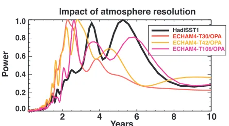
Impact of atmosphere resolution
2 4 6 8 10
Years
0.0 0.2 0.4 0.6 0.8 1.0
Po
wer
HadISST1
[image:18.595.309.545.592.722.2]ECHAM4-T30/OPA ECHAM4-T42/OPA ECHAM4-T106/OPA
Figure. 1: Different Spectra of the El-Niño phenomenon for different representations of the atmosphere in coupled Atmosphere-Ocean Global Circulation Model runs. From Guilyardi, 2003.
The Program for Integrated Earth System Modelling (PRISM) and the European Network for Earth System Modelling (ENES)
Guy P. Brasseur1, Reinhard G. Budich1, and Gerbrand
Komen2
1Max-Planck-Institut für Meteorologie, Hamburg,
Germany
2KNMI, De Bilt, The Netherlands
corresponding e-mail: [email protected]
The development of climate models has been an important milestone towards the quantitative assessment of human-driven perturbations in the Earth system. Complex models have been developed in several research centres in Europe, North America and Japan. These models have been evaluated, inter-compared, and used for various assessments including those performed by the Intergovernmental Panel for Climate Change (IPCC). In spite of the large efforts conducted by the scientific community during the last decades, many processes are still poorly represented in climate models, so that large uncertainties still exist in current models. These are often related to the way sub - grid processes (i.e., cloud and convective processes, precipitation, ocean eddies, etc.) are parameterized. Ensembles of multi-model integrations should help quantify these uncertainties and should provide a sense of the probability that a specific climate prediction may occur. Several groups are already developing the statistical methodologies needed to conduct and interpret such ensemble integrations.
Running codes by combining different model components developed in different institutions is an important aspect of the strategy developed in Europe. To achieve such a goal, model components need to be interchangeable without major efforts. This is being achieved by developing common physical interfaces that follow certain pre-established specifications. The PRISM Project (Program for Integrated Earth System Modelling1), an infrastructure project supported by the
European Commission, is precisely designed to facilitate the exchanges of component models, and to integrate complex Earth System models under chosen configurations on different supercomputing platforms. The “science of model coupling” remains a challenging problem, as illustrated for example by Figure 1. Coupling different state-of-the-art atmospheric general circulation models with different ocean models leads, for example, to very different representations of the El Niño events. Issues related to the coupling of model components will become even more crucial as nonlinear biological and chemical processes are fully implemented in complex Earth system models (Figure 2).
PRISM was established following recommendations made in a Euroclivar report published in November 1998. This report called for increased cooperation between the different climate modelling centres in Europe, and suggested that model development consortia be established to perform model inter-comparisons and improve parameterizations. The exchange of software and model results was encouraged, and the need for a large European climate computing facility to perform long high-resolution multi-model ensemble integrations was identified. The objective of PRISM is therefore to develop a flexible model structure with interchangeable model components that can exchange information through standard interfaces and through a universal coupler. As a result, the European scientific community will adopt a common software framework for model development, model diagnostics and visualization. When completed, this infrastructure will become available to the scientific community. PRISM is coordinated by the Max-Planck-Institute for Meteorology in Germany, jointly with the Royal Netherlands Meteorological Institute.
What has soon become clear is that, beside the development of common software infrastructures, the various European centres must increase their scientific cooperation, and share a common vision for future research. The purpose of the European Network for Earth System Modelling (ENES - http://www/enes.org) is to facilitate exchanges of ideas and to develop new scientific and support initiatives. ENES includes more than 50 partners representing the academic world, national research centres, meteorological services, computing centres, and industry. The ultimate objective of ENES is to accelerate progress towards a better understanding of the processes governing the Earth system and towards the development of improved predictive capability. The ENSEMBLES project, recently approved by the European
1 Funded by the European Commission under contract
Commission, will address important scientific issues in support of the ENES objectives. ENSEMBLES, which includes 72 partners, is co-ordinated by the Hadley Centre in the UK.
[image:19.595.52.288.80.253.2]One issue addressed by ENES is the lack of sufficient computing resources available in Europe to maintain a high level of climate modelling activities, and to contribute world-class science. Japan and the US have Figure. 2: The PRISM configuration
Atmosphere Atmospheric
Chemistry
Land Surface
Sea Ice
Ocean Biogeochemistry
Ocean
Regional Climate Coupler
Pascale Braconnot1, Sylvie Joussaume1, Sandy
Harrison2, Chris Hewitt3, Paul Valdes2, Gilles Ramstein1,
Ronald J. Stouffer4, Bette Otto-Bliesner5 and Karl
Taylor6.
1 IPSL/LSCE, Gif-sur-Yvette, France 2 University of Bristol, Bristol, UK 3 Hadley Centre, Met Office, Exeter, UK 4 GFDL, Princeton, USA
5 NCAR, Boulder, USA
6 PCMDI, LLNL, Livermore, USA
email: [email protected]
The Paleoclimate Intercomparison Project (PMIP) is a long-standing initiative endorsed by the World Climate Research Programme (WCRP; JSC/CLIVAR Working Group on Coupled Modelling (WGCM)) and the International Geosphere - Biosphere Programme (IGBP; Past Global Changes (PAGES)). The major goals of PMIP are to determine ability of models to reproduce climate states that are different from those of today and to increase our understanding of climate change. The PMIP effort developed out of a NATO Advanced Research Workshop, convened in 1991, which led to a cooperative and coordinated effort to compare model simulations with each other and with paleoclimatic data. The mid-Holocene and the Last Glacial Maximum were the major targets during the first phase of PMIP both for modelling and data synthesis. Simulating the mid-Holocene represents a sensitivity experiment to increased seasonal
The second phase of the Paleoclimate Modeling Intercomparison Project (PMIP-II)
been developing strategic views on the question of hardware infrastructure. Europe must also establish its strategy, despite the complex institutional situation and the lack of a dedicated project by European industry in this respect. New climate assessments will require more complex and higher resolution models. Model integrations will cover longer time periods, and involve multi-model ensemble runs. Over the last decades, Europe has developed a strong intellectual capability in its research centres and universities, and has provided important scientific information to decision-makers. It will be able to contribute efficiently to future assessments and to decisions related to climate policy only if it maintains a strong research activity with the appropriate supercomputing infrastructure. Figure 3 (page 1) illustrates the processes that lead to more integrative Earth system models, and the associated level of computer resources that will be needed to develop and use these models in the future.
Reference
Guilyardi, E., S. Gualdi, J.M. Slingo, A. Navarra, P. Delecluse, J. Cole, G. Madec, M. Roberts, M. Latif, and L. Terray, 2003: Representing El Niño in coupled ocean-atmosphere GCMs: the dominant role of the atmosphere. J. Climate, submitted.
contrast of incoming solar radiation at the top of the atmosphere in the northern hemisphere, which leads to enhanced summer monsoons in the tropics. On the other hand, simulating the Last Glacial Maximum, allows an assessment of model representation of extreme cold conditions as well as feedbacks arising from a reduced CO2 concentration and 2 to 3 km ice sheet elevation over
North America and northern Europe. Only atmospheric models were considered in the first phase. PMIP results formed a crucial part of the evaluation of climate models in the Third Assessment Report of the Intergovernmental Panel on Climatic Changes (IPCC, 2001)
is needed to increase our confidence in future climate projections. In addition new periods of interest have emerged. Some of the PMIP participants are interested in the Early Holocene, when the insolation forcing was even larger than during the mid-Holocene, and in glacial inception studies to better constrain the major feedbacks that are needed to amplify the insolation forcing and bring the system from a warm interglacial state to a cold glacial state.
This second phase of PMIPII is just starting. It was initiated at an international PMIP workshop in Cambridge last year (Harrison et al., 2002). In this new phase of the project, we will study the role of climate feedbacks arising in the different climate subsystems (atmosphere, ocean, land surface, sea ice and land ice) and evaluate the capability of state of the art climate models to reproduce climate states that are radically different from those of today. PMIPII is led by Sylvie Joussaume, Laboratoire des Sciences du Climat et de l’Environnement, France, email: [email protected], and will have five modelling foci:
•
the mid-Holocene climate (contact: Pascale Braconnot, Laboratoire des Sciences du Climat et de l’Environnement, France,email: [email protected])
•
the last glacial maximum climate (contact: Chris Hewitt, Met Office Hadley Centre, UK;email: [email protected])
•
the Early Holocene climate (contact: Paul Valdes, University of Bristol, UK;email: [email protected])
•
the last glacial inception (contact: Gilles Ramstein, Laboratoire des Sciences du Climat et de l’Environnement, France,email: [email protected])
•
a sensitivity experiment to water hosing in the north Atlantic (contact: Ronald J. Stouffer, NOAA Geophysical Fluid Dynamics Laboratory, USA; email: [email protected]). This experiment is a common experiment between PMIP and WGCM’s Coupled Model Intercomparison Project (CMIP). Analyses will be based on model–model and model-data comparisons. Evaluation of model experiments depends on the existence of spatially explicit data sets that can be compared with output from the model simulations. PMIPII will continue to stimulate continuous development and improvement of paleo-environmental data sets (contact: Sandy